| Issue |
A&A
Volume 642, October 2020
|
|
|---|---|---|
| Article Number | A208 | |
| Number of page(s) | 14 | |
| Section | Interstellar and circumstellar matter | |
| DOI | https://doi.org/10.1051/0004-6361/202038749 | |
| Published online | 22 October 2020 | |
Interstellar oxygen along the line of sight of Cygnus X-2★
1
SRON Netherlands Institute for Space Research,
Sorbonnelaan 2,
3584
CA
Utrecht,
The Netherlands
e-mail: This email address is being protected from spambots. You need JavaScript enabled to view it.
2
Anton Pannekoek Astronomical Institute, University of Amsterdam,
PO Box 94249,
1090 GE
Amsterdam,
The Netherlands
3
Debye Institute for Nanomaterials Science, Utrecht University,
Universiteitsweg 99,
3584 CG
Utrecht,
The Netherlands
4
Astrophysikalisches Institut und Universitats-Sternwärte (AIU),
Schillergäßchen 2-3,
07745
Jena,
Germany
5
Ciencia de los Materiales e Ingeniería Metalúrgica y Química Inorgánica, Universidad de Cadiz, Cadiz, Spain
6
Academia Sinica, Institute of Astronomy and Astrophysics,
11F Astronomy-Mathematics Building, NTU/AS campus, No. 1, Section 4, Roosevelt Rd.,
Taipei
10617,
Taiwan
Received:
24
June
2020
Accepted:
10
September
2020
Abstract
Interstellar dust permeates our Galaxy and plays an important role in many physical processes in the diffuse and dense regions of the interstellar medium (ISM). High-resolution X-ray spectroscopy, coupled with modelling based on laboratory dust measurements, provides a unique probe for investigating the interstellar dust properties along our line of sight towards Galactic X-ray sources. Here, we focus on the oxygen content of the ISM through its absorption features in the X-ray spectra. To model the dust features, we perform a laboratory experiment using the electron microscope facility located at the University of Cadiz in Spain, where we acquire new laboratory data in the oxygen K-edge. We study 18 dust samples of silicates and oxides with different chemical compositions. The laboratory measurements are adopted for our astronomical data analysis. We carry out a case study on the X-ray spectrum of the bright low-mass X-ray binary Cygnus X-2, observed by XMM−Newton. We determine different temperature phases of the ISM and parameterise oxygen in both gas (neutral and ionised) and dust form. We find Solar abundances of oxygen along the line of sight towards the source. Due to both the relatively low depletion of oxygen into dust form and the shape of the oxygen cross section profiles, it is challenging to determine the precise chemistry of interstellar dust. However, silicates provide an acceptable fit. Finally, we discuss the systematic discrepancies in the atomic (gaseous phase) data of the oxygen edge spectral region using different X-ray atomic databases as well as consider future prospects for studying the ISM with the Arcus concept mission.
Key words: astrochemistry / X-rays: individuals: Cygnus X-2 / dust, extinction / X-rays: binaries / X-rays: ISM
Data for the calculated dust extinction cross sections are only available at the CDS via anonymous ftp to cdsarc.u-strasbg.fr (130.79.128.5) or via http://cdsarc.u-strasbg.fr/viz-bin/cat/J/A+A/642/A208
© ESO 2020
1 Introduction
The composition of the interstellar medium (ISM) is very important for the evolution of the Galaxy and for star formation processes. In particular, interstellar dust (ID) is an important constituent of our Galaxy as it can control the temperature of the ISM and it is the catalyst for the formation of complex molecules (Mathis 1990).
The dust chemical and physical properties in the diffuse ISM are not yet fully understood. Observations show that ID in the diffuse ISM is not spatially homogeneous (e.g. Planck Collaboration XXVI 2011; Planck Collaboration XXV 2011; Ysard et al. 2015). Silicate grains are an important and abundant component of ID and can be found in many different stages of the life cycle of stars (Henning 2010). It is believed to be mainly produced in oxygen-rich asymptotic giant branch stars (Gail et al. 2009) but also in novae and supernovae type II (Wooden et al. 1993; Rho et al. 2008) and young stellar objects (Nittler et al. 1997). On the other hand, carbonaceous grains could form in interstellar clouds as carbon grains likely have shorter lifetimes (Jones & Nuth 2011).
The physical and chemical properties of silicate dust have been historically studied along different directions in the Galaxy at wavelengths ranging from radio to the ultraviolet (Draine & Li 2001; Dwek et al. 2004). It is believed that elements such as O, Fe, Si, and Mg form the cosmic silicates, which represent most of the dust mass in the ISM (Mathis 1998). Further evidence for such elements to be locked up in dust is the fact that they are depleted from the gaseous phase (Henning 2010; Savage & Sembach 1996; Jenkins 2009).
Oxygen is one of the most abundant and important elements for life on Earth. However, the total budget of oxygen in the diffuse and dense ISMs cannot be fully explained yet (Whittet 2010). Jenkins (2009) reported that the oxygen in the diffuse interstellar gas is being depleted at a rate that cannot be associated with only silicates and metallic oxides. They found that the total fraction of the missing oxygen is not compatible with the stoichiometric ratios of even the most oxygen-rich silicate compounds. This requires some contribution of additional compounds.
It has also been proposed that oxygen must be locked up in molecules together with elements with a high cosmic abundance such as CO, CO2, and O2 (Jenkins 2009). These oxygen-bearing molecules have small but non-negligible abundances (van Dishoeck 2004). Additionally, van Dishoeck et al. (1998) found that, close to young stellar objects, for large extinction values, oxygen atoms are found in the form of water. Whittet et al. (1988), Eiroa & Hodapp (1989) and Smith et al. (1993) found that the strength of the 3.05 μm water ice feature becomes much weaker as the extinction decreases. Later on, Whittet et al. (2001) showed that the same feature becomes detectable for extinction when larger than 3.2 and increases linearly with increasing extinction above that value.
High-resolution X-ray spectroscopy is a powerful tool for unveiling the physical and chemical properties of the diffuse ISM (Wilms et al. 2000; Lee & Ravel 2005; Lee 2009; de Vries & Costantini 2009; Pinto et al. 2013; Corrales et al. 2016; Schulz et al. 2016; Zeegers et al. 2017, 2019; Rogantini et al. 2018). It provides the possibility of studying the composition of cosmic dust in different environments of the ISM through the study of absorption features of gas and dust. In particular, X-ray absorption fine structures (XAFSs) are unique fingerprints of dust. When an X-ray photon excites a core electron (n = 1), the outward-moving photo-electron will interact with the neighbouring atoms. This interaction will modify the wave function of the photo-electron due to constructive and destructive interferences. In this way, the absorption probability will be modified in a unique pattern that depends on the configuration of the neighbouring atoms. Therefore, the shape ofXAFSs can be used to determine the chemical structure of dust (see also Newville 2004 for further explanation).
The oxygen K-edge region has already been explored using observations from the XMM−Newton and Chandra satellites. Costantini et al. (2012) and Pinto et al. (2010) find that about 15–25% of the total neutral oxygen is in dust. On the other hand, Gatuzz et al. (2014) suggest that the oxygen edge can be fitted only with gaseous oxygen. Later, Eckersall et al. (2017) studied the gas features in the oxygen K-edge region with the models used in Gatuzz et al. (2015). They noticed strong residuals in the fit and noted that they are likely due to dust. Furthermore, Joachimi et al. (2016) searched for evidence of CO in XMM−Newton spectra of low-mass X-ray binaries and suggested two weak detections.
In the literature, there are different studies regarding the atomic data in the oxygen K-edge region. Theoretical calculations on the K-shell photo-absorption of oxygen ions have been performed by García et al. (2005) and McLaughlin & Kirby (1998) using the R-matrix approach. Moreover, laboratory measurements have been carried out in order to determine the absolute energy of the photo-absorption cross sections of oxygen ions (Menzel et al. 1996; Stolte et al. 1997). Gorczyca et al. (2013) present an analytical formula to describe with accuracy the photo-absorption cross section of O I in X-ray spectral modelling, and Leutenegger et al. (2020) discuss an experimental technique for the determination of the absolute calibration of the oxygen Kα transition energy. Finally, Frati et al. (2020) review the oxygen K-edge X-ray absorption spectra of atoms, molecules, and solids, where the oxygen 1s core electron is excited to the lowest empty states at ~ 530 eV.
In order to determine the presence of dust in the oxygen K-edge, we need to use accurate dust models. To this end, we performed a laboratory measuring campaign to compute the absorption cross sections of 18 dust compounds with different chemical compositions, such as different types of silicates and oxides. In order to investigate the crystallinity, our samples contain both crystalline and amorphous dust grains. From studies of the 10 μm silicate feature in the mid-infrared band, it has been found that the stoichiometry of silicate dust is mostly amorphous olivines (Mg2-xFexSiO4) and pyroxenes (Mg1-xFexSiO3) (Kemper et al. 2004; Min et al. 2007). Additionally, Kemper et al. (2004) found that towards SgrA*, most silicates have an amorphous structure and fewer than 2.2% are crystalline. They also reported that ~85% of the amorphous grains are olivines and ~15% are pyroxenes. The pyroxenes are found to be slightly Mg-rich with Mg/(Mg+Fe) ~0.55, while the olivines may be Fe-rich. Min et al. (2007) concluded that the amorphous silicates are Mg-rich with Mg/(Mg+Fe) ~0.9. They also found that the crystallinity in the ISM is small, and they report a pure crystalline forsterite grain composition (Mg2 SiO4). Moreover, experimental studies of astrophysical dust analogues with application to infrared observations have been presented by Nuth et al. (2002).
We apply the new dust models to the high-resolution XMM−Newton Reflection Grating Spectrometer (RGS) spectrum of Cygnus X-2 in order to study the oxygen K-edge spectral region. It is a bright X-ray source with a moderate column density (~ 2 × 1021 cm−2, Juett 2004) and high flux (2.3 × 10⁻⁹ erg s−1 cm−2 in the 0.3–2 keV band). Cygnus X-2 has been proposed as a Z-track source (Hasinger & van der Klis 1989) and is believed to reach the Eddington luminosity limit during its high state (Bałucińska-Church et al. 2010; Mondal et al. 2018; King & Ritter 1999). The distance of the source has been estimated to be around 7–12 kpc, and its galactic coordinates are l, b = 87.°33–11.°32, which means that it is located about 1.4–2.4 kpc away from the Galactic plane (Cowley et al. 1979; McClintock et al. 1984; Smale 1998; Yao et al. 2009). The systemic velocity of the binary system was found to be about −220 km s−1 (Cowley et al. 1979; Casares et al. 1998).
Previous studies of Cygnus X-2 with Chandra gratings showed that the oxygen region is possibly mildly absorbed by ID (Yao et al. 2009). Moreover, Juett (2004) studied the Chandra high-energy transmission grating (HETGS) spectrum of Cygnus X-2 and noted that features from dust or molecular compounds are not essential for obtaining a good fit. The goal of this investigation is to understand the contribution of dust to the oxygen K-edge spectral region using up-to-date laboratory and atomic data measurements.
The paper is organised as follows. In Sect. 2, we describe the dust samples used in this work, the laboratory experiment, and the treatment of the laboratory data. In Sect. 3 and Appendix A, we present the methodology used to calculate the dust extinction cross sections for the oxygen K-edge. In Sect. 4, we apply the new models to the RGS spectrum of Cygnus X-2. The discussion of our results is presented in Sect. 5, and in Sect. 5.3 we compare the results obtained using both the atomic databases ofSPEX and XSTAR for the O I, O II, and O III lines. In Sect. 6, we discuss the prospects of observing the oxygen K-edge region with the Arcus concept mission. In Sect. 7, we present our conclusions.
2 The laboratory experiment
2.1 The dust samples
The dust samples used in this work are laboratory analogues of silicates and oxides of astronomical interest. The choice of samples reflects the astronomical silicate composition that has been discussed in previous studies (Jaeger et al. 1998; Kemper et al. 2004; Chiar & Tielens 2006; Min et al. 2007; Olofsson et al. 2009; Draine & Lee 1984). In Table 1, we present the list of the samples. The first column shows the reference number of each sample. In the second and third columns, we present the compound name and its chemical formula and, in the last column, its form (i.e. crystalline or amorphous). We note that in this paper we use amorphous as a collective term to describe all non-crystalline materials. Our amorphous samples are glassy, and their structures may still show a short-range order of atoms. However, Si K-edge spectra of our amorphous samples show a smooth profile, significantly distinct from the crystal ones (Zeegers et al. 2019).
Most of the compounds have already been presented in previous works, in which the Mg-, Fe-, and Si K-edges have been measured in the laboratory using the Synchrotron facilities (Zeegers et al. 2017, 2019; Rogantini et al. 2018). Among the samples, four of them are natural (samples 2, 7, 9, and 16 in Table 1) and six are commercial products (samples 11, 12, 13, 15, 17, and 18). The rest of the silicate samples are synthesised in the laboratories at the Astrophysikalisches Institut, Universitats-Stenwarte (AIU), and Osaka University (for details see Zeegers et al. 2019).
Our list of 18 samples contains pyroxenes, olivines, and oxides. The silicate samples consist of different Mg/(Mg+Fe) ratios, between 0.5 and 0.9, and can be found in both amorphous and crystalline form. We also include magnesium-pure compounds such as forsterite and enstatite (samples 7, 8, and 11) and the iron-pure compound named fayalite (sample 10). Additionally, we have three different types of quartz (samples 16, 17, and 18), one in crystalline form and two in different stages of amorphisation.
Dust samples.
2.2 The electron energy loss measurements
We performed laboratory measurements of dust in the oxygen K-edge using the STEM (Scanning Transmission Electron Microscope)facility at the University of Cadiz. Electron energy loss spectroscopy (EELS) is a technique that measures the change in the kinetic energy of electrons after the interaction with the sample. This provides structural and chemical information on the material studied. The interaction between the incident electron beam and the materials, in our case the dust samples, results in electron energy loss. A typical energy loss spectrum contains many features and is separated into three spectral regions. The “zero-loss” peak represents electrons that are transmitted without suffering measurable energy loss. The “low-loss” spectrum corresponds to electrons that have interacted with the weakly bound electrons of the atoms, and, finally, the “core-loss” region contains the electrons that have interacted with the tightly bound core electrons (Egerton 2011). The core-loss region contains the information on the fine structures of dust, also referred to as energy loss near edge structures (ELNES). Both ELNES and XAFS present exactly the same spectral shape under the dipole approximation.
For the purpose of this experiment, we used the Titan Cubed Themis 60–300 microscope in the STEM mode, operating at 200 keV. In parallel, high-spatial resolution EELS experiments were performed with the spectrum-imaging mode, which allows the correlation of analytical and structural information on selected regions of the studied material. In this way, we compared the information of the spectra with those of the spatial distribution of the sample. These supporting information experiments were acquired in dual EELS mode using an energy dispersion of 0.25 eV, 50 pA probe current, and 50 ms acquisition time per EELS spectrum (Manzorro et al. 2019).
The STEM mode of the electron microscope enables us to scan the dust samples pixel by pixel. The resulting spectrum will be the average spectrum of each pixel. To improve the signal-to-noise ratio of our data, we obtained five to ten measurements of individual selected regions of interest on the dust sample.
2.3 Analysing the laboratory data
In this section, we describe the analysis of the raw laboratory measurements step by step. We used the python library hyperspy1 to convert the laboratory data to a python-readable format.
Thickness selection
The dust samples have an intrinsic thickness variation. In the EELS, as the thickness of the area under study increases, the strong interaction of the primary electrons within the grain will result in multiple scattering events. This tends to reduce the signal-to-noise ratio of the EELS edges. To this end, we needed to apply a selection criterion. We selected the part of the grain that belongs to thinner regions and then considered the total spectrum of this part (see Fig. 1). In most cases, we excluded the part of the grain with  >1, where t is the thickness of the sample and
  the mean free path of the inelastic scattering.
Spectrum alignment
An important correction in the EELS measurements is the alignment of the energy axis of the spectrum. For this reason, we obtained the low-loss spectrum that contains the zero loss peak (Egerton 2011). The zero loss peak is a sharp peak with an energy loss of zero that appears in an EELS spectrum. We obtained this spectrum for every measurement.
Background subtraction
Next, we removed the EELS background by fitting a polynomial to the data.
Testing energy calibration uncertainties
In laboratory experiments, one needs to be careful regarding the absolute energy of the measured edges. It is possible that the calibration of the instrument is not perfect, and therefore a verification of the absolute energy values has to be done. Consequently, we tested the position of the oxygen edges with a reference feature that appears in our measurements. This narrow feature is a pre-peak of the oxygen edge, and it is associated with an electron transition into molecular oxygen (O2), which is thought to evaporate due to the impact of the incident electron beam and the sample. We adopted a value of 530.5 eV for the absolute energy of the O2 transition (Jiang & Spence 2006; Garvie 2010).
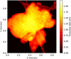 |
Fig. 1 Example of the region of interest of the dust sample obtained from laboratory data. The colourbar of the image indicates thethickness ratio |


Principal component analysis
We performed a principal component analysis (PCA) to further test if the samples are homogeneous in composition and thickness. The original idea of PCA was established by Karl Pearson in 1901 (Pearson 1901). The PCA is a statistical procedure that uses anorthogonal transformation to find inhomogeneity in a set of data. It decomposes a dataset into a set of orthogonal eigenvectors or principal components. When the PCA is applied to a set of spectra, the result is a set of spectral components that describe thevariability of the data. The first principal component is the eigenvector that corresponds to the data with the maximum variation. The second eigenvector will show the second highest variation of the data, and it is orthogonal to the first one. Every principal component will reveal the characteristic features of the spectrum in order of variation.
The dust grains may present inhomogeneities. Using the PCA, we crosschecked if the selected area on the grain is homogeneous. If it was not homogeneous, we repeated the analysis for this specific measurement. This procedure is useful for obtaining robust results and avoiding artefacts in the spectra.
3 From laboratory measurements to cross sections
From the EELS experiment, we obtained the information about the fine structure of dust for each sample. Next, we need to calculate the extinction cross section in order to adopt the laboratory measurements for astronomical data analysis. The methodology we used has been described extensively in previous works of Zeegers et al. (2017) and Rogantini et al. (2018). Here, we discuss the main steps of this analysis, adjusted for the oxygen K-edge.
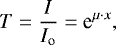
When the X-ray light passes through a material, it can be either transmitted, absorbed, or scattered. The transmittance of a material is the amount of light that is transmitted, and it is described by the Beer-Lambert law:
 (1)
(1)
where I is the transmitted light and Io the incident light intensity. In the above equation, μ is the attenuation coefficient inμm−1, which depends on the properties of the material, and x describes the depth of the radiation in the material (i.e. the thickness of the sample in μm). The thickness should be two to three times less than the attenuation length to avoid the thickness effects that can reduce the XAFS amplitude (Parratt et al. 1957; Bunker 2010). For the attenuation length, we used the tabulated values obtained from the Center for X-Ray Optics (CXRO) at the Lawrence Berkeley National Laboratory2. In this work, we chose a thickness of 0.05 μm for all our samples, a necessary value in order to calculate the optical constants. This is consistent with the mean value values of the EELS thickness of our samples, which vary from ~0.01 to ~0.09 μm.
In Fig. 2, we present the transmittance of an olivine compound obtained using the EELS. The pre-edge (<0.525 keV) and the post-edge (>0.575 keV) have been fitted to the tabulated values from the CXRO (Henke et al. 1993).
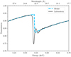 |
Fig. 2 Transmission spectrum in the oxygen K-edge using an amorphous olivine dust compound (solid black line). The dashed blueline indicates the tabulated data found in Henke et al. (1993), which were used to fit the pre-edge and post-edge of the data. |
3.1 Optical constants
In order to calculate the total extinction cross section of our samples, we needed to first determine the optical constants of the complex refractive index, which is defined as:
 (2)
(2)
The refractive index is a complex number that describes how the light propagates into a material. The real part shows the dispersive behaviour on the incident light and the imaginary part its absorption. In the literature, there are different notations to describe the optical constants (Rogantini et al. 2018).
The imaginary part (k) can be calculated directly from the data and the thickness of each sample from the equations:
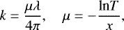 (3)
(3)
where λ represents the wavelength of the incident X-ray and T the transmittance. Knowing the imaginary part of the refractive index, we used the Kramers-Kronig relations to calculate the real part. The Kramers-Kronig relations are mathematical relations that connect the real and imaginary parts of any complex function. These relations are used to calculate the real part from the imaginary part (or vice versa) of functions in physical systems. Here, to calculate the real part, we used the python package kkcalc3. This tool uses the optical constants in terms of atomic scattering factors, f1 and f2, which are described in Watts 2014 (see also Rogantini et al. 2018). In Fig. 3, we present the optical constants for the amorphous olivine (compound #1).
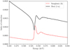 |
Fig. 3 Real and imaginary parts of the refractive index calculated using the Kramers-Kronig relations for the amorphous olivine. |
3.2 Total extinction cross section
Once the optical constants n and k have been calculated, one can proceed to the calculation of the total extinction cross section. To calculate the extinction cross section, we applied the Mie theory (Mie 1908). Therefore, we used the python module miepython4, which is the python version of the MIEV0 code described in Wiscombe (1980).
The Mie code calculates the extinction and scattering efficiency factors (Q). Then, the scattering, extinction, and absorption cross sections are calculated from the efficiency factors of each grain of radius r (C =πr2Q). However, the ID grains can be found in different sizes in the ISM. To obtain the total scattering, extinction, and absorption cross sections, one needs to integrate over a grain size distribution:
 (4)
(4)
where n(r) is the size distribution. We used the Mathis-Rumpl-Nordsieck model (MRN; Mathis et al. 1977):
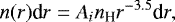 (5)
(5)
where nH is the number density of H atoms and Ai is a normalisation constant that depends on the type of dust. The normalisation constant is calculated using the equations described in Mauche & Gorenstein (1986) and Hoffman & Draine (2016). For the purpose of this paper, we calculated the extinction cross section to be implemented into the amol model of the software package SPEctral X-ray and the UV modelling and analysis (SPEX), version 3.05.005 (Kaastra et al. 1996, 2018).
In Fig. 4, we present the calculated extinction, absorption, and scattering cross sections for amorphous olivines. In Appendix A, we present the extinction cross sections for all compounds used in this work. The oxygen compounds measured in the laboratory show a smooth absorption profile. Contrary to the Si K-edge (Zeegers et al. 2019), the differences among the different types of silicates are negligible. However, we note a difference between the amorphous and crystalline structure of the same compound. This effect is due to the different configuration of the atoms in the grain.
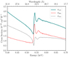 |
Fig. 4 Calculated extinction (σext), absorption (σabs), and scattering (σsca) cross section of dust per hydrogen nucleus. The figure shows the amorphous olivine composition in the oxygen K-edge region. |
4 Application to the astronomical data
X-ray spectra of X-ray binaries can be used to study the ISM in several lines of sight in the Galaxy through the absorption features of dust and gas. Thus, we implemented the laboratory data into a complete spectral model and applied them to Cygnus X-2, an ideal X-ray targetfor studying the composition of the interstellar oxygen. For this analysis, we used data from the RGS on board the XMM−Newton satellite (den Herder et al. 2001). The RGS has a resolving power of 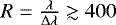 and an effective area of ~45 cm2 around the oxygen K-edge.
4.1 Data reduction
We reduced the XMM−Newton data using the Science Analysis Software (SAS, version.16). First, we ran the rgsproc command tocreate the event lists. Then, we filtered the RGS event lists for flaring particle background using the default value of 0.2 counts s−1 threshold. We also excluded the bad pixels using keepcool=no in the SAS task rgsproc. We used four long observations in total, which are listed in Table 2. In bright sources, some areas of the grating data may be affected by pile-up. In order to recognise the spectral regions not affected by pile-up, one can compare the first and the second order for each grating (Costantini et al. 2012). We have negligible pile-up in all the observations used in this paper. The spectral shape does not vary significantly through different epochs, and this allows us to combine the data using the SAS command rgscombine to obtain a higher signal-to-noise ratio (S/N).
XMM−Newton observation log.
4.2 Spectral fitting
In Fig. 5, we present the stacked RGS spectrum of Cygnus X-2. The spectrum displays narrow absorption features near the oxygen (~23 Å), neon (~13.5 Å), and iron (~17.5 Å) edges, which are produced byionised gas in the ISM. In this work, we mainly focus on the neutral and mildly ionised gas. We fitted the spectrum in the range of 10–35 Å using SPEX. To evaluate the goodness of our fit, we adopted C-Statistics, which is denoted as Cstat in the rest of the manuscript. SPEX uses Cstat as describedin Cash (1979) but with an addition that allows an estimate of the goodness of the fit (for details, see Kaastra 2017). Additionally, in our analysis we used the proto-Solar abundance units from Lodders & Palme (2009).
The continuum emission of low-mass X-ray binaries originates from their accretion disc and corona and may be described asa blackbody and a Comptonised emission component, respectively (see Done et al. 2007). As the RGS provides a relatively narrow energy band, the full shape of the spectral energy distribution cannot be constrained. Thus, we used a simple power law model (pow in SPEX), which reproduces the continuum shape in the RGS band well.
4.2.1 The gas phase modelling
We further adopted a neutral gas component (hot model in SPEX) to absorb the continuum. The hot model calculates the transmission of a plasma in collisional ionisation equilibrium (de Plaa et al. 2004). For a given temperature and set of abundances, the model calculates the ionisation balance and then determines all the ionic column densities by scaling to the prescribed total hydrogen column density. At low temperatures (~0.5 eV), the hot model effectively represents the neutral gas since this temperature is sufficiently low to obtain neutral species. In this model, both the hydrogen column density and the temperature (eV) are free parameters. This provides a physical fit of the ISM because we can distinguish between the different temperature phases along this line of sight.
We needa total of three hot componentsto fit the weakly and mildly ionised features. These correspond to three different ISM temperatures along this line of sight: a quasi-neutral gas component with kT ~ 0.7 eV, a warmer component with kT ~ 2.5 eV, and a hotterone with kT ~ 12 eV (Fig. 6). The parameters of the fit are shown in Table 3. We limited the temperaturerange of the cold gas to a maximum of 0.7 eV in order to have the cold gas phase dominated by neutral oxygen.
The stacked spectrum of Cygnus X-2 presents additional features: some absorption-like features around 24–25 Å and a “bump” around 24–26 Å. The strongest absorption-like features are at 24.7 and 24.3 Å, and their positions do not correspond to lines from known ions. In fact, they correspond to absorption features in the effective area of the RGS. We conclude that these dips are most likely due to calibration issues associated with bad pixels and can therefore be ignored.
Moreover, the bump in the continuum around 24–26 Å is too narrow to be associated with any continuum components. A similar bump is also observed after the Fe L-edge (around 18 Å). These excesses have been associated with broad line emission features (Madej et al. 2010, 2014). For the improvement of our modelling, we fitted this excess with Gaussian profiles in order to prevent residuals in the oxygen edge region from a badly fitted continuum and uncertainties in the determination of the absorption parameters. Thus, we leave the interpretation on the nature of these bumps open.
Best fit parameters for Cygnus X-2.
4.2.2 The oxygen edge region
Here, we focus our analysis on the oxygen edge spectral region (19−26 Å), which displays several sharp absorption features. We followed a similar fitting procedure for the oxygen edge as in Costantini et al. (2012). The best fit is shown in the top panel of Fig. 6, and in the lower panel we present the contribution of each absorption component. The 0.7 eV gas (see Sect. 4.2.1) imprints the line from O I at 23.5 Å and is mimicking the neutral gas. At this stage, we obtain Cstat = 1702 for 786 degrees of freedom (d.o.f.) from our fit. At shorter wavelengths, the gas component with a higher temperature of kT = 2.5 eV produces the absorption by O II (23.36 Å). A third component with a slightly smaller contribution to the total fit takes into account the O III absorption line together with some weaker O IV and O V lines. At wavelengths 22, 21.6, and 18.9 Å, the lines of O VI, O VII, and O VIII, respectively, are the signature of an even hotter phase of the ISM. We took the absorption by this hot gas into account using the slab model in SPEX. This model calculates absorption by a slab of optically thin gas, where the column density of ions are fitted individually and are independent of each other (see Table 4). The additional hot models and the slab model improve our fit, and we obtain Cstat/d.o.f. = 1380/772.
Finally, we tested the effect of our new calculated dust extinction cross sections implemented into the amol model of SPEX. We let the column density of the amol model free to vary as well as the depletion of the hot model (hot #1, cold phase) of oxygen and iron. The depletion of silicon was fixed to 90% according to the literature (Rogantini et al. 2019; Zeegers et al. 2019), and the depletion of magnesium was constrained to be at least 80%.
In Fig. 6, we present the best fit using an olivine dust compound (amorphous olivine, compound #1 in Table 1). In the lower panel of Fig. 6, we present the transmission of the dust component (in magenta). As shown, the transmission of the dust covers a broad area of the oxygen K-edge spectral region from about 22.3 to 22.5 Å. By adding the dust model, we obtain Cstat/d.o.f. = 1342/771.
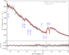 |
Fig. 5 Top panel: XMM−Newton RGS spectrum of the low-mass X-ray binary Cygnus X-2 and the best fit model. Lower panel: residuals of the best fit model, where (O-M)/M is (Observed-Model)/Model. |
Best fit parameters of the slab component.
4.3 The dust modelling
Our fit takes into account the contribution of dust using the newly calculated extinction models. The analysis above was carried out using an amorphous (glassy) olivine composition (MgFeSiO4). However, the ISM consists of a mixture of chemical elements. We further tested different combinations of dust compounds that contain silicates and oxides from the list in Table 1 to search for the best fit combination that describes the ID composition in the oxygen edge. The amol model in SPEX allows us to test four different compounds at a time. The number of different combinations is given by the equation:
 (6)
(6)
where e is the number of the available edge profiles and c the combination class (see also Costantini et al. 2012). In our fit, we did not include the aluminium compounds (Table 1, compounds #12 and 13) since this element is outside the RGS energy band and it is believed that they exist in small quantities in the ISM. We did our fit with the remaining 16 compounds, which gives 1820 different combinations.
To compare the different models, we used a robust statistical approach. The standard model comparison tests (such as the χ2 goodness-of-fit test) cannot be used because our models are not nested (Protassov et al. 2002). Therefore, we performed the Akaike information criterion (AIC), which represents a robust and fast way to select the models that have more support from the data (Akaike 1974), as explained in detail in Rogantini et al. (2019). The AIC gives the relative quality of statistical models for a given set of data.
We calculated the AIC difference (ΔAIC) over all candidate models with respect to the model that has the lowest AIC value. The most significant model is the one that minimises the AIC value. Using the criteria of Burnham & Anderson (2002), the models with ΔAIC > 10 can be ruled out. From the 1820 total models we obtained using the different combinations, about 590 of them were found with ΔAIC > 10 and were therefore excluded. These models contain mostly quartz (compounds #16, 17, and 18 in Table 1). The rest of the models, with ΔAIC < 10, are plausible representations of the data. In particular, models with ΔAIC < 2 can fit the oxygen edge equally well. We obtained 311 different models with ΔAIC < 2. We conclude that we do not have sufficient resolution to distinguish between the different dust samples. The modelling is further complicated by the relative similarity of the oxygen absorption dust profiles measured in the laboratory (Appendix A).
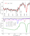 |
Fig. 6 Top panel: XMM−Newton RGS spectrum of the low-mass X-ray binary Cygnus X-2 and the best fit around the oxygen K-edge. Lower panel: transmission of each component. The transmission of the colder component of the ISM has been multiplied by a factor of 2.5 for display purposes. |
5 Discussion
5.1 The multi-phase gas in the ISM
The study of the ISM through the X-ray absorption features of bright background sources, such as X-ray binaries, is a unique tool for probing the different phases of the ISM. By studying the oxygen K-edge spectral region, we can constrain different gas temperatures by probing low and high ionisation gas, covering O I to O VII. With our modelling, we find a column density of oxygen in the gas phase of ~ 1.27 × 1018 cm−2, which corresponds to (93 ± 9)% of the total column density. The remaining (7 ± 1)% corresponds to solid phase (dust) with a column density of ~9 × 1016 cm−2. Consideringthe errors, if the percentage is lower or higher than 100%, this implies that there is an under- or over-abundance of oxygen relative to the assumed abundances.
In our modelling, the gas consists of three components (see Table 3). We have a cold gas component with temperature kT = 0.7 eV (or T ~8 × 10³ K), a warm component with kT = 2.5 eV (or T ~ 3 × 10⁴ K), and a hot component with kT = 12 eV (or T ~ 14 × 104 K).
In Table 5, we present the column density of each oxygen ion and its contribution to the total column density. The cold component produces mainly O I, some of which is locked into dust. The warm component produces the low ionisation absorption line (O II), and the hotter component produces the O III, O IV, and O V. The higher ionisation lines are reproduced using a slab model in SPEX.
Molecules such as carbon monoxide are expected to be found in the ISM, especially in molecular clouds. It has been proposed that the missing oxygen from the gas phase of the ISM could be locked up in molecules together with elements with a high cosmic abundance such as CO (Jenkins 2009). To test for the presence of carbon monoxide, we used the cross section (Barrus et al. 1979) implemented into the amol model in SPEX. According to this model, such a feature is expected to be present around 23.2 Å. We obtained an upper limit of NCO < 3.2 × 1016 cm−2, which corresponds to less than 2% of the total oxygen.
Contributions to the total oxygen column density.
5.2 Abundances and depletions
From the best fit of Cygnus X-2, we find a column density of neutral hydrogen of NH= (1.9 ± 0.1) × 1021 cm−2. This is in agreement with the hydrogen column density along this line of sight (HI4PI Collaboration 2016). We find that (7 ± 1)% of the oxygen is depleted into dust. Pinto et al. (2010) studied the ISM along the line of sight of GS 1826-238 and found that (10 ± 2)% of oxygen is contained within solids such as silicates and water ice. Later, Costantini et al. (2012) studied the absorbed spectrum of 4U 1820-30 and found (20 ± 2)% depletion. Our best fit indicates that the amount of oxygen in gas and dust is consistent with Solar composition. The results on the abundances and depletions are presented in Table 6.
5.3 Comparison between the atomic databases for oxygen
Accurate high-resolution X-ray spectroscopy and interpretation require state-of-the-art atomic databases. The oxygen K-edge region is one of the most important and complicated astrophysical spectral regions. The available atomic X-ray databases for atomic oxygen are based on different cross section calculations.
Here, we compared the photo-absorption cross sections implemented into SPEX (Kaastra et al. 1996) and XSTAR (Kallman & Bautista 2001) for the atomic oxygen O I, O II, and O III. We further examined the effect of the different atomic databases in our fitting of the oxygen edge region of the ISM.
Regarding XSTAR, the O I photo-absorption cross section can be found in Gorczyca et al. (2013); for O II and O III, it uses the R-matrix calculations from García et al. (2005).
For the inner K-shell transitions of oxygen ions, SPEX uses the calculations provided by E. Behar (HULLAC calculations). For O I and O II, the lines are shifted in order to match the Juett (2004) observational values (see Kaastra et al. 2010). Moreover, the oscillator strengths and transition rates for all O I lines have been updated with values computed by Ton Raassen using Cowan’s code (Cowan 1981, T. Raassen priv. comm.). In Appendix B, we present the wavelengths and oscillator strengths of the oxygen lines implemented in SPEX.
In Fig. 7, we present the comparison between the different atomic databases in the oxygen K-edge region. The top panel shows the model calculations for the atomic transitions of O I. The cross sections of O I agree with one another regarding the wavelengths of the lines. The middle panel of Fig. 7 refers to O II and the bottom panel to O III. For O II and O III, the absolute energy of the lines between SPEX and XSTAR is in disagreement.
We further tested how the discrepancy between the atomic databases can affect the spectral fitting of Cygnus X-2. We substituted the atomic lines of SPEX for O I, O II, and O III with those of XSTAR. This enabled us to fit the lines of these three ions with the XSTAR atomic data. In order to do that, we used the musr model, which allows external models in SPEX. We fitted the stacked spectrum of Cygnus X-2 using the lines for O I, O II, and O III from the musr model. We kept the same modelling as described in Sect. 4.2.1, as well as the slab and the amol model. The free parameter of the musr model in our case is the column density and is fitted independently for each individual O I, O II, and O III ion. We kept the ratio of the column density of these three ions consistent with the ratio of the column densities and temperatures in the hot model in SPEX in order to set a physical fit. In Fig. 8, we present the best fit results. The XSTAR database gives a better fit around 22.7 Å. We notice that there is a weaker transition of O I in that region, and, using the XSTAR database, we obtain reduced residuals. In the rest of the spectrum, we achieve a similar fit.
Oxygen column densities and abundances.
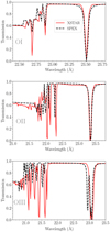 |
Fig. 7 Comparison of the atomic databases of SPEX and XSTAR at the oxygen K-edge for O I (top panel), O II (middle panel), and O III (bottom panel). |
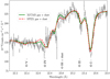 |
Fig. 8 Fitting the oxygen K-edge region using different atomic databases for the oxygen (O I, O II, and O III). The plot compares the fits using the XSTAR and SPEX atomic databases. The dust compound used here is the amorphous olivine. |
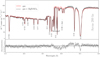 |
Fig. 9 Simulated data of Cygnus X-2 in the oxygen K-edge using the Arcus response matrix. Top panel: simulated spectrum according to our best fit model (Sect. 4.2.2), which includes dust (dashed black line). The solid red line shows the Arcus simulation without including a dust model. Bottom panel: residuals of the fit with the gas-only model. |
6 Prospects of the oxygen K-edge study with the Arcus-concept mission
Future missions may provide us with suitable instruments to study the ISM in the soft X-rays (<1 keV). For example, the Arcus-concept mission (Smith 2016) will provide higher-resolution data with a resolving power of R ~ 3000.
We performed an Arcus simulation in order to understand if we can put better constrains on the properties of the ISM and distinguish between the gas and solid phases. We used the XMM−Newton RGS best fitmodel in the oxygen edge region described in Sect. 4.2.2 as a template to simulate an Arcus spectrum of Cygnus X-2. This model contains both gas and dust. In Fig. 9, we present the Arcus simulation with an exposure time of 200 ks.
We tested the effects of including or excluding dust in our spectrum by fitting a gas-only model (red line). It is clear from the shape of the model around 23.2 Å that we willbetter distinguish the effect of dust in the oxygen K-edge with Arcus. Additionally, the wealth of individually resolved lines will place stronger constraints on the exact structure of the multi-phase gas. In general, new X-ray missions such as ATHENA and XRISM and concept missions such as Arcus will open up new frontiers to help us better understand the physics of the ISM (e.g. Rogantini et al. 2018; Costantini et al. 2019; Corrales et al. 2019).
7 Conclusions
In this work, we present a set of laboratory measurements in the O K-edge region, and we aim to characterise the absorption properties of silicates and oxides that likely form the ID content. We measured 18 different dust species, including silicates and oxides, and we calculated the dust extinction cross sections. We adopted the laboratory data for astronomical data analysis, and, in particular, we implemented the dust models into the SPEX X-ray fitting package. We further modelled the XMM−Newton RGS spectrum of Cygnus X-2 using the existing models of gas in SPEX and the new laboratory data. We focused our analysis on the oxygen K-edge region in order to study the dust and the properties of the multi-phase ISM along the line of sight to the source. We further discussed the effect of using different atomic databases for the atomic oxygen, and, finally, we commented on new frontiers in the oxygen K-edge from the future concept mission of Arcus. Our main results are the following:
-
from the oxygen K-edge, we are able to study the multi-phase gas. We probe different gas temperatures and disentangle lower and higher ionised gas components, such as O I and O VIII;
-
the absorption spectrum of Cygnus X-2 shows the presence of gas and dust in the oxygen K-edge region. We find that (93 ± 9)% of the total amount of oxygen is in the gas phase, while a smaller amount of (7 ± 1)% is found in dust;
-
the oxygen abundance along the line of sight of Cygnus X-2 is consistent with proto-Solar values. This could be due to the fact that Cygnus X-2 is located farther from the Galactic centre compared to other X-ray binaries;
-
to fully study the dust in the oxygen K-edge, we need instruments with higher resolution and effective area, such as the Arcus-concept mission. This will help minimise the statistical noise and better distinguish between the gas and solid phases;
-
accurate atomic databases are necessary in order to accurately study the oxygen region. The importance of the atomic data is highlighted in view of future X-ray missions.
Acknowledgements
We would like to thank our referee J. Nuth for the useful suggestions. I.P., M.M., D.R. and E.C. are supported by the Netherlands Organisation for Scientific Research (NWO) through The Innovational Research Incentives Scheme Vidi grant 639.042.525. The Space Research Organization of the Netherlands is supported financially by the NWO. The authors would like to thank E. Gatuzz for providing the cross section calculations of the atomic oxygen implemented into XSTAR, J. Garcia for valuable suggestions on atomic data and J. Wilms, R. Smith for useful information about Arcus. We thank J. de Plaa for helping with the musr model in SPEX and J. Kaastra for general instructions regarding SPEX. We also thank M. Diaz Trigo for useful information regarding Cygnus X-2.
Appendix A: Dust extinction cross sections in the oxygen K-edge
We present the calculated dust extinction cross sections in the oxygen K-edge. The cross sections were calculated from laboratory data of 18 dust samples with different chemical compositions. The resolution of the laboratory measurements is 0.25 eV.
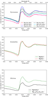 |
Fig. A.1 Calculated dust extinction cross sections. The symbol a refers to amorphous compounds and c to crystalline. |
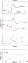 |
Fig. A.2 Calculated dust extinction cross sections. The symbol a refers to amorphous compounds and c to crystalline. |
Appendix B: Atomic oxygen lines in SPEX
In the following tables, we present the wavelength, energy, and oscillator strength of the atomic oxygen lines (O I, O II, and O III) implemented into SPEX.
O I lines implemented into SPEX.
O II lines implemented into SPEX.
O III lines implemented into SPEX.
References
- Akaike, H. 1974, IEEE Trans. Auto. Control, 19, 716 [Google Scholar]
- Bałucińska-Church, M., Gibiec, A., Jackson, N. K., & Church, M. J. 2010, A&A, 512, A9 [NASA ADS] [CrossRef] [EDP Sciences] [Google Scholar]
- Barrus, D. M., Blake, R. L., Burek, A. J., Chambers, K. C., & Pregenzer, A. L. 1979, Phys. Rev. A, 20, 1045 [NASA ADS] [CrossRef] [Google Scholar]
- Bunker, G. 2010, Introduction to XAFS (Cambridge U.K: Cambridge University Press) [CrossRef] [Google Scholar]
- Burnham, K. P., & Anderson, D. R. 2002, Model Selection and Multimodel Inference: a Practical Information-theoretic Approach (Springer) [Google Scholar]
- Casares, J., Charles, P., & Kuulkers, E. 1998, ApJ, 493, L39 [NASA ADS] [CrossRef] [Google Scholar]
- Cash, W. 1979, ApJ, 228, 939 [NASA ADS] [CrossRef] [Google Scholar]
- Chiar, J. E., & Tielens, A. G. G. M. 2006, ApJ, 637, 774 [NASA ADS] [CrossRef] [Google Scholar]
- Corrales, L. R., García, J., Wilms, J., & Baganoff, F. 2016, MNRAS, 458, 1345 [NASA ADS] [CrossRef] [Google Scholar]
- Corrales, L., Valencic, L., Costantini, E., et al. 2019, BAAS, 51, 264 [Google Scholar]
- Costantini, E., Pinto, C., Kaastra, J. S., et al. 2012, A&A, 539, A32 [NASA ADS] [CrossRef] [EDP Sciences] [Google Scholar]
- Costantini, E., Zeegers, S. T., Rogantini, D., et al. 2019, A&A, 629, A78 [NASA ADS] [CrossRef] [EDP Sciences] [Google Scholar]
- Cowan, R. 1981, The Theory of Atomic Structure and Spectra, Los Alamos Series in Basic and Applied Sciences (California: University of California Press) [Google Scholar]
- Cowley, A. P., Crampton, D., & Hutchings, J. B. 1979, ApJ, 231, 539 [NASA ADS] [CrossRef] [Google Scholar]
- de Plaa, J., Kaastra, J. S., Tamura, T., et al. 2004, A&A, 423, 49 [NASA ADS] [CrossRef] [EDP Sciences] [Google Scholar]
- de Vries, C. P., & Costantini, E. 2009, A&A, 497, 393 [NASA ADS] [CrossRef] [EDP Sciences] [Google Scholar]
- den Herder, J. W., Brinkman, A. C., Kahn, S. M., et al. 2001, A&A, 365, L7 [NASA ADS] [CrossRef] [EDP Sciences] [Google Scholar]
- Done, C., Gierliński, M., & Kubota, A. 2007, A&ARv, 15, 1 [NASA ADS] [CrossRef] [EDP Sciences] [Google Scholar]
- Draine, B. T., & Lee, H. M. 1984, ApJ, 285, 89 [Google Scholar]
- Draine, B. T., & Li, A. 2001, ApJ, 551, 807 [NASA ADS] [CrossRef] [Google Scholar]
- Dwek, E., Zubko, V., Arendt, R. G., & Smith, R. K. 2004, ASP Conf. Ser., 309, 499 [Google Scholar]
- Eckersall, A. J., Vaughan, S., & Wynn, G. A. 2017, MNRAS, 471, 1468 [CrossRef] [Google Scholar]
- Egerton, R. 2011, Electron Energy-Loss Spectroscopy in the Electron Microscope (Boston MA: Springer) 3rd Edition [CrossRef] [Google Scholar]
- Eiroa, C., & Hodapp, K. W. 1989, A&A, 210, 345 [NASA ADS] [Google Scholar]
- Frati, F., Hunault, M. O. J. Y., & de Groot, F. M. F. 2020, Chem. Rev., 120, 4056 [CrossRef] [Google Scholar]
- Gail, H. P., Zhukovska, S. V., Hoppe, P., & Trieloff, M. 2009, ApJ, 698, 1136 [NASA ADS] [CrossRef] [Google Scholar]
- García, J., Mendoza, C., Bautista, M. A., et al. 2005, ApJS, 158, 68 [NASA ADS] [CrossRef] [Google Scholar]
- Garvie, L. 2010, Am. Mineral., 95, 92 [CrossRef] [Google Scholar]
- Gatuzz, E., García, J., Mendoza, C., et al. 2014, ApJ, 790, 131 [NASA ADS] [CrossRef] [Google Scholar]
- Gatuzz, E., García, J., Kallman, T. R., Mendoza, C., & Gorczyca, T. W. 2015, ApJ, 800, 29 [NASA ADS] [CrossRef] [Google Scholar]
- Gorczyca, T. W., Bautista, M. A., Hasoglu, M. F., et al. 2013, ApJ, 779, 78 [NASA ADS] [CrossRef] [Google Scholar]
- Hasinger, G., & van der Klis, M. 1989, A&A, 225, 79 [NASA ADS] [Google Scholar]
- Henke, B. L., Gullikson, E. M., & Davis, J. C. 1993, At. Data Nucl. Data Tables, 54, 181 [NASA ADS] [CrossRef] [Google Scholar]
- Henning, T. 2010, ARA&A, 48, 21 [NASA ADS] [CrossRef] [Google Scholar]
- HI4PI Collaboration (Ben Bekhti, N., et al.) 2016, A&A, 594, A116 [NASA ADS] [CrossRef] [EDP Sciences] [Google Scholar]
- Hoffman, J., & Draine, B. T. 2016, ApJ, 817, 139 [NASA ADS] [CrossRef] [Google Scholar]
- Jaeger, C., Molster, F. J., Dorschner, J., et al. 1998, A&A, 339, 904 [Google Scholar]
- Jenkins, E. B. 2009, ApJ, 700, 1299 [NASA ADS] [CrossRef] [Google Scholar]
- Jiang, N., & Spence, J. 2006, Ultramicroscopy, 106, 215 [CrossRef] [Google Scholar]
- Joachimi, K., Gatuzz, E., García, J. A., & Kallman, T. R. 2016, MNRAS, 461, 352 [CrossRef] [Google Scholar]
- Jones, A. P., & Nuth, J. A. 2011, A&A, 530, A44 [NASA ADS] [CrossRef] [EDP Sciences] [Google Scholar]
- Juett, A. M. 2004, AAS Meeting Abstracts, 205, 41.04 [Google Scholar]
- Kaastra, J. S. 2017, A&A, 605, A51 [NASA ADS] [CrossRef] [EDP Sciences] [Google Scholar]
- Kaastra, J. S., Mewe, R., & Nieuwenhuijzen, H. 1996, in UV and X-ray Spectroscopy of Astrophysical and Laboratory Plasmas (Cambridge: Cambridge University Press), 411 [Google Scholar]
- Kaastra, J. S., Raassen, T., & de Vries, C. 2010, in The Energetic Cosmos: from Suzaku to ASTRO-H, 70 [Google Scholar]
- Kaastra, J. S., Raassen, A. J. J., de Plaa, J., & Gu, L. 2018, https://doi.org/10.5281/zenodo.2419563 [Google Scholar]
- Kallman, T., & Bautista, M. 2001, ApJS, 133, 221 [NASA ADS] [CrossRef] [Google Scholar]
- Kemper, F., Vriend, W. J., & Tielens, A. G. G. M. 2004, ApJ, 609, 826 [NASA ADS] [CrossRef] [Google Scholar]
- King, A. R., & Ritter, H. 1999, MNRAS, 309, 253 [NASA ADS] [CrossRef] [Google Scholar]
- Lee, J. 2009, Chandra’s First Decade of Discovery, eds. S. Wolk, A. Fruscione, & D. Swartz, 58 [Google Scholar]
- Lee, J. C., & Ravel, B. 2005, ApJ, 622, 970 [NASA ADS] [CrossRef] [Google Scholar]
- Leutenegger, M. A., Kühn, S., Micke, P., et al. 2020, PRL, submitted [arXiv:2003.13838] [Google Scholar]
- Lodders, K., & Palme, H. 2009, Meteorit. Planet. Sci. Suppl., 72, 5154 [Google Scholar]
- Madej, O. K., Jonker, P. G., Fabian, A. C., et al. 2010, MNRAS, 407, L11 [NASA ADS] [Google Scholar]
- Madej, O. K., García, J., Jonker, P. G., et al. 2014, MNRAS, 442, 1157 [CrossRef] [Google Scholar]
- Manzorro, R., Celín, W. E., Pérez-Omil, J. A., Calvino, J. J., & Trasobares, S. 2019, ACS Catal., 9, 5157 [CrossRef] [Google Scholar]
- Mathis, J. S. 1990, ARA&A, 28, 37 [NASA ADS] [CrossRef] [Google Scholar]
- Mathis, J. S. 1998, ApJ, 497, 824 [NASA ADS] [CrossRef] [Google Scholar]
- Mathis, J. S., Rumpl, W., & Nordsieck, K. H. 1977, ApJ, 217, 425 [NASA ADS] [CrossRef] [Google Scholar]
- Mauche, C. W., & Gorenstein, P. 1986, ApJ, 302, 371 [NASA ADS] [CrossRef] [Google Scholar]
- McClintock, J. E., Remillard, R. A., Petro, L. D., Hammerschlag-Hensberge, G., & Proffitt, C. R. 1984, ApJ, 283, 794 [NASA ADS] [CrossRef] [Google Scholar]
- McLaughlin, B. M., & Kirby, K. P. 1998, J. Phys. B At., Mol. Opt. Phys., 31, 4991 [NASA ADS] [CrossRef] [Google Scholar]
- Menzel, A., Benzaid, S., Krause, M. O., et al. 1996, Phys. Rev. A, 54, R991 [NASA ADS] [CrossRef] [PubMed] [Google Scholar]
- Mie, G. 1908, Ann. Phys., 330, 377 [Google Scholar]
- Min, M., Waters, L. B. F. M., de Koter, A., et al. 2007, A&A, 462, 667 [NASA ADS] [CrossRef] [EDP Sciences] [Google Scholar]
- Mondal, A. S., Dewangan, G. C., Pahari, M., & Raychaudhuri, B. 2018, MNRAS, 474, 2064 [CrossRef] [Google Scholar]
- Newville, M. 2004, Consortium for Advanced Radiation Sources (University of Chicago), 78, http://xafs.org [Google Scholar]
- Nittler, L. R., Alexander, O., Gao, X., Walker, R. M., & Zinner, E. 1997, ApJ, 483, 475 [NASA ADS] [CrossRef] [Google Scholar]
- Nuth, Joseph A., I., Rietmeijer, F. J. M., & Hill, H. G. M. 2002, Meteorit. Planet. Sci., 37, 1579 [NASA ADS] [CrossRef] [Google Scholar]
- Olofsson, J., Augereau, J. C., van Dishoeck, E. F., et al. 2009, A&A, 507, 327 [NASA ADS] [CrossRef] [EDP Sciences] [Google Scholar]
- Parratt, L. G., C. F., Hempstead, & Jossem, E. L. 1957, Phys. Rev., 105, 1228 [NASA ADS] [CrossRef] [Google Scholar]
- Pearson, K. 1901, Lond. Edinb. Dublin Philos. Mag. J. Sci., 2, 559 [Google Scholar]
- Pinto, C., Kaastra, J. S., Costantini, E., & Verbunt, F. 2010, A&A, 521, A79 [NASA ADS] [CrossRef] [EDP Sciences] [Google Scholar]
- Pinto, C., Kaastra, J. S., Costantini, E., & de Vries, C. 2013, A&A, 551, A25 [NASA ADS] [CrossRef] [EDP Sciences] [Google Scholar]
- Planck Collaboration XXV. 2011, A&A, 536, A25 [NASA ADS] [CrossRef] [EDP Sciences] [Google Scholar]
- Planck Collaboration XXVI. 2011, A&A, 536, A26 [NASA ADS] [CrossRef] [EDP Sciences] [Google Scholar]
- Protassov, R., van Dyk, D. A., Connors, A., Kashyap, V. L., & Siemiginowska, A. 2002, ApJ, 571, 545 [NASA ADS] [CrossRef] [Google Scholar]
- Rho, J., Kozasa, T., Reach, W. T., et al. 2008, ApJ, 673, 271 [NASA ADS] [CrossRef] [Google Scholar]
- Rogantini, D., Costantini, E., Zeegers, S. T., et al. 2018, A&A, 609, A22 [NASA ADS] [CrossRef] [EDP Sciences] [Google Scholar]
- Rogantini, D., Costantini, E., Zeegers, S. T., et al. 2019, A&A, 630, A143 [CrossRef] [EDP Sciences] [Google Scholar]
- Savage, B. D., & Sembach, K. R. 1996, ARA&A, 34, 279 [NASA ADS] [CrossRef] [Google Scholar]
- Schulz, N. S., Corrales, L., & Canizares, C. R. 2016, ApJ, 827, 49 [NASA ADS] [CrossRef] [Google Scholar]
- Smale, A. P. 1998, ApJ, 498, L141 [NASA ADS] [CrossRef] [Google Scholar]
- Smith, R. K., Abraham, M. H., Allured, R., et al. 2016, SPIE Conf. Ser., 9905, 99054M [Google Scholar]
- Smith, R. G., Sellgren, K., & Brooke, T. Y. 1993, MNRAS, 263, 749 [NASA ADS] [CrossRef] [Google Scholar]
- Stolte, W. C., Lu, Y., Samson, J. A. R., et al. 1997, J. Phys. B At. Mol. Phys., 30, 4489 [NASA ADS] [CrossRef] [Google Scholar]
- van Dishoeck, E. F. 2004, ARA&A, 42, 119 [NASA ADS] [CrossRef] [Google Scholar]
- van Dishoeck, E. F., Helmich, F. P., Schutte, W. A., et al. 1998, ASP Conf. Ser., 132, 54 [Google Scholar]
- Watts, B. 2014, Opt. Exp., 22, 23628 [NASA ADS] [CrossRef] [Google Scholar]
- Whittet, D. C. B. 2010, ApJ, 710, 1009 [NASA ADS] [CrossRef] [Google Scholar]
- Whittet, D. C. B., Bode, M. F., Longmore, A. J., et al. 1988, MNRAS, 233, 321 [NASA ADS] [CrossRef] [Google Scholar]
- Whittet, D. C. B., Gerakines, P. A., Hough, J. H., & Shenoy, S. S. 2001, ApJ, 547, 872 [NASA ADS] [CrossRef] [Google Scholar]
- Wilms, J., Allen, A., & McCray, R. 2000, ApJ, 542, 914 [NASA ADS] [CrossRef] [Google Scholar]
- Wiscombe, W. J. 1980, Appl. Opt., 19, 1505 [NASA ADS] [CrossRef] [PubMed] [Google Scholar]
- Wooden, D. H., Rank, D. M., Bregman, J. D., et al. 1993, ApJS, 88, 477 [NASA ADS] [CrossRef] [Google Scholar]
- Yao, Y., Schulz, N. S., Gu, M. F., Nowak, M. A., & Canizares, C. R. 2009, ApJ, 696, 1418 [NASA ADS] [CrossRef] [Google Scholar]
- Ysard, N., Köhler, M., Jones, A., et al. 2015, A&A, 577, A110 [NASA ADS] [CrossRef] [EDP Sciences] [Google Scholar]
- Zeegers, S. T., Costantini, E., de Vries, C. P., et al. 2017, A&A, 599, A117 [NASA ADS] [CrossRef] [EDP Sciences] [Google Scholar]
- Zeegers, S. T., Costantini, E., Rogantini, D., et al. 2019, A&A, 627, A16 [NASA ADS] [CrossRef] [EDP Sciences] [Google Scholar]
All Tables
All Figures
|
Fig. 1 Example of the region of interest of the dust sample obtained from laboratory data. The colourbar of the image indicates thethickness ratio |
| In the text | |
|
Fig. 2 Transmission spectrum in the oxygen K-edge using an amorphous olivine dust compound (solid black line). The dashed blueline indicates the tabulated data found in Henke et al. (1993), which were used to fit the pre-edge and post-edge of the data. |
| In the text | |
|
Fig. 3 Real and imaginary parts of the refractive index calculated using the Kramers-Kronig relations for the amorphous olivine. |
| In the text | |
|
Fig. 4 Calculated extinction (σext), absorption (σabs), and scattering (σsca) cross section of dust per hydrogen nucleus. The figure shows the amorphous olivine composition in the oxygen K-edge region. |
| In the text | |
|
Fig. 5 Top panel: XMM−Newton RGS spectrum of the low-mass X-ray binary Cygnus X-2 and the best fit model. Lower panel: residuals of the best fit model, where (O-M)/M is (Observed-Model)/Model. |
| In the text | |
|
Fig. 6 Top panel: XMM−Newton RGS spectrum of the low-mass X-ray binary Cygnus X-2 and the best fit around the oxygen K-edge. Lower panel: transmission of each component. The transmission of the colder component of the ISM has been multiplied by a factor of 2.5 for display purposes. |
| In the text | |
|
Fig. 7 Comparison of the atomic databases of SPEX and XSTAR at the oxygen K-edge for O I (top panel), O II (middle panel), and O III (bottom panel). |
| In the text | |
|
Fig. 8 Fitting the oxygen K-edge region using different atomic databases for the oxygen (O I, O II, and O III). The plot compares the fits using the XSTAR and SPEX atomic databases. The dust compound used here is the amorphous olivine. |
| In the text | |
|
Fig. 9 Simulated data of Cygnus X-2 in the oxygen K-edge using the Arcus response matrix. Top panel: simulated spectrum according to our best fit model (Sect. 4.2.2), which includes dust (dashed black line). The solid red line shows the Arcus simulation without including a dust model. Bottom panel: residuals of the fit with the gas-only model. |
| In the text | |
|
Fig. A.1 Calculated dust extinction cross sections. The symbol a refers to amorphous compounds and c to crystalline. |
| In the text | |
|
Fig. A.2 Calculated dust extinction cross sections. The symbol a refers to amorphous compounds and c to crystalline. |
| In the text | |
Current usage metrics show cumulative count of Article Views (full-text article views including HTML views, PDF and ePub downloads, according to the available data) and Abstracts Views on Vision4Press platform.
Data correspond to usage on the plateform after 2015. The current usage metrics is available 48-96 hours after online publication and is updated daily on week days.
Initial download of the metrics may take a while.