| Issue |
A&A
Volume 642, October 2020
|
|
|---|---|---|
| Article Number | A176 | |
| Number of page(s) | 13 | |
| Section | Extragalactic astronomy | |
| DOI | https://doi.org/10.1051/0004-6361/201937146 | |
| Published online | 15 October 2020 | |
The chemical evolution of the dwarf spheroidal galaxy Sextans⋆,⋆⋆
1
Physics Institute, Laboratory of Astrophysics, Ecole Polytechnique Fédérale de Lausanne (EPFL), 1290 Sauverny, Switzerland
e-mail: This email address is being protected from spambots. You need JavaScript enabled to view it.
2
GEPI, Observatoire de Paris, Université PSL, CNRS, Place Jules Janssen, 92190 Meudon, France
3
Institute of Astronomy, University of Cambridge, Madingley Road, Cambridge CB3 0HA, UK
4
Instituto de Astrofísica de Canarias (IAC), Calle Via Láctea, s/n, 38205 San Cristóbal de la Laguna, Tenerife, Spain
5
Departamento de Astrofísica, Universidad de La Laguna, 38206 San Cristóbal de la Laguna, Tenerife, Spain
6
Laboratoire Lagrange, Université de Nice Sophia-Antipolis, Observatoire de la Côte d’Azur, Nice, France
7
Kapteyn Astronomical Institute, University of Groningen, Landleven 12, 9747 AD Groningen, The Netherlands
8
Department of Physics and Astronomy, University of Victoria, PO Box 3055, STN CSC, Victoria, BC V8W 3P6, Canada
9
European Southern Observatory, Alonso de Cordova 3107, Vitacura, Casilla 19001, Santiago, Chile
10
European Southern Observatory, Schwarzschild-Str. 2, 85748 Garching, Germany
11
McDonald Observatory, University of Texas at Austin, Fort David, TX, USA
Received:
19
November
2019
Accepted:
24
March
2020
Abstract
We present our analysis of the FLAMES dataset targeting the central 25′ region of the Sextans dwarf spheroidal galaxy (dSph). This dataset is the third major part of the high-resolution spectroscopic section of the ESO large program 171.B-0588(A) obtained by the Dwarf galaxy Abundances and Radial-velocities Team. Our sample is composed of red giant branch stars down to V ∼ 20.5 mag, the level of the horizontal branch in Sextans, and allows users to address questions related to both stellar nucleosynthesis and galaxy evolution. We provide metallicities for 81 stars, which cover the wide [Fe/H] = −3.2 to −1.5 dex range. The abundances of ten other elements are derived: Mg, Ca, Ti, Sc, Cr, Mn, Co, Ni, Ba, and Eu. Despite its small mass, Sextans is a chemically evolved system, showing evidence of a contribution from core-collapse and Type Ia supernovae as well as low-metallicity asymptotic giant branch stars (AGBs). This new FLAMES sample offers a sufficiently large number of stars with chemical abundances derived with high accuracy to firmly establish the existence of a plateau in [α/Fe] at ∼0.4 dex followed by a decrease above [Fe/H] ∼ −2 dex. These features reveal a close similarity with the Fornax and Sculptor dSphs despite their very different masses and star formation histories, suggesting that these three galaxies had very similar star formation efficiencies in their early formation phases, probably driven by the early accretion of smaller galactic fragments, until the UV-background heating impacted them in different ways. The parallel between the Sculptor and Sextans dSph is also striking when considering Ba and Eu. The same chemical trends can be seen in the metallicity region common to both galaxies, implying similar fractions of SNeIa and low-metallicity AGBs. Finally, as to the iron-peak elements, the decline of [Co/Fe] and [Ni/Fe] above [Fe/H] ∼ −2 implies that the production yields of Ni and Co in SNeIa are lower than that of Fe. The decrease in [Ni/Fe] favours models of SNeIa based on the explosion of double-degenerate sub-Chandrasekhar mass white dwarfs.
Key words: stars: abundances / galaxies: dwarf / galaxies: evolution
Tables 2–6, 9–13 are only available at the CDS via anonymous ftp to cdsarc.u-strasbg.fr (130.79.128.5) or via http://cdsarc.u-strasbg.fr/viz-bin/cat/J/A+A/642/A176
Based on the ESO Program 171.B-0588(A).
© ESO 2020
1. Introduction
A large variety of topics rely on our understanding of the formation and evolution of dwarf galaxies. In the ΛCDM cosmology, galaxies form hierarchically by cooling and condensation of the baryons within dark-matter haloes that gradually merge (White & Rees 1978). Strong efforts are therefore concentrated on counting, characterising, and quantifying the impact of the earliest and smallest of these galactic systems from the local universe to the reionisation period (e.g. Tolstoy et al. 2009; Wise et al. 2014; Sawala et al. 2016; Simon 2019; Torrealba et al. 2019).
The Sextans dwarf spheroidal galaxy (dSph) was discovered by Irwin et al. (1990). At a distance of ∼90 kpc, it is one of the closest satellites of the Milky Way (Mateo et al. 1995; Lee et al. 2003; Battaglia et al. 2011). Its late discovery is the consequence of its large extent on the sky with a tidal radius of 120 ± 20 arcmin (Cicuéndez et al. 2018) and low surface brightness of σ0 = 18.2 ± 0.5 mag arcmin−2 (Irwin & Hatzidimitriou 1995) making it a challenging galaxy to characterise given the large fraction of Milky Way interlopers.
The analysis of the colour magnitude diagram (CMD) of Sextans reveals a stellar population which is largely dominated by stars older than ∼11 Gyr (Lee et al. 2009), with evidence for radial metallicity and age gradients, the oldest stars forming the most spatially extended component (Lee et al. 2003; Battaglia et al. 2011; Okamoto et al. 2017; Cicuéndez et al. 2018).
Spectroscopic follow-up in Sextans started in 1991 at medium–low resolution in the region of the calcium triplet (CaT, 8498, 8542 and 8662 Å). Da Costa et al. (1991) identified six galaxy members and derived a mean metallicity of [Fe/H] = −1.7 ± 0.25 dex. Suntzeff et al. (1993) increased the sample of galaxy members up to 43 and revised the galaxy peak metallicity to −2.05 ± 0.04 dex. The enhanced multiplexing power of a new generation of spectrographs with over ∼30′ fields of view opened up the possibility to analyse hundreds of stars at once. Spectroscopy in the region of the Mg I triplet (5140−5180 Å) and the CaT absorption features were used for rough chemical tagging and to investigate the mass profile of Sextans, as well as the possible existence of kinematically distinct stellar populations at its centre (Walker et al. 2006, 2009; Battaglia et al. 2011). Sextans is thought to be about 0.4 Gyr away from its pericentre (rperi ∼ 75 kpc) moving towards its apocentre (rapo ∼ 132 kpc), and its orbit seems inconsistent with a membership to the vast polar structure of Galactic satellites (Casetti-Dinescu et al. 2018; Fritz et al. 2018). Until recently, no statistically significant distortions or signs of tidal disturbances had been found down to very low surface brightness limit (Cicuéndez et al. 2018), but combined reanalysis of the spectroscopic membership and deep photometry have revealed the presence of a ring-like structure that is interpreted as the possible sign of a merger (Cicuéndez & Battaglia 2018).
One thread of studies traces the formation and evolution of galaxies by exploring their chemical evolution as preserved in stellar abundance patterns. Comparison between galaxies of very different star formation histories also offers important insight into poorly understood nucleosynthetic origins such as for the neutron capture elements (e.g. Tolstoy et al. 2009; Jablonka et al. 2015; Mashonkina et al. 2017; Ji et al. 2019; Reichert et al. 2020). Here, spectroscopic multiplex again plays a fundamental role allowing to switch from the pioneer ensembles of a few stars per galaxy that had elemental abundances and abundance ratios (e.g. Hill et al. 1995; Shetrone et al. 2001, 2003) to statistically significant samples. A step forward arose from Keck/DEIMOS medium-resolution (R ∼ 7000) spectroscopy, with about 35 Sextans stars with delivered abundances of α-elements (Mg, Si, Ca, Ti) at accuracies better than 0.3 dex (Kirby et al. 2011). This sample has recently been completed with Cr, Co, and Ni abundances (Kirby et al. 2018). The number of remaining open questions in Sextans is nevertheless very large. In particular, its low metallicity range ([Fe/H] ≤ −2.) is still uncovered. Only a few extremely metal-poor stars have been targeted in this galaxy (Aoki et al. 2009; Tafelmeyer et al. 2010). The mean trend and scatter at fixed [Fe/H] of the abundance ratios still need to be investigated over the full chemical evolution of Sextans.
The VLT/FLAMES fibre-spectrograph has already been transformative in addressing similar questions in other dSphs. The Dwarf Abundances and Radial velocity team (DART) targeted the Fornax and Sculptor dSphs (Letarte et al. 2010; Hill et al. 2019). The present paper presents the DART high-resolution spectroscopic sample of Sextans. In the following, we present the analysis of a sample of 81 Sextans stars that have been observed in the central region of Sextans at high resolution (R ∼ 20 000) with VLT/FLAMES (GIRAFFE and UVES). This is the largest sample of red giant branch (RGB) stars dedicated to a chemical analysis, and allows us to address questions related to both stellar nucleosynthesis and galaxy evolution.
2. Observations and data reduction
Our targets are RGBs located in the central 25′ field of the Sextans dSph. About half of the sample is composed of RGBs previously identified as Sextans members based on their radial velocities measured from medium-resolution spectra around the calcium triplet (Battaglia et al. 2011). The rest of the sample was selected from the position of the stars in the CMD of Sextans. The spatial distribution of our sample stars is presented in Fig. 1, while Fig. 2 displays their location along the RGB V versus V − I plane.
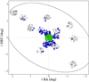 |
Fig. 1. Spatial distribution of the DART spectroscopic observations in Sextans. The grey points show the stars observed around the CaT survey (Battaglia et al. 2011). The blue circles correspond to the probable members of this medium-resolution sample, while the green points are the stars of our high-resolution sample (see Table 2 for the values of RA and Dec). The black ellipse represents the tidal radius of Sextans calculated by Cicuéndez et al. (2018). |
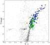 |
Fig. 2. Colour-magnitude diagram of the Sextans stars. The blue and green points are in as in Fig. 1. The black dots correspond to Sextans photometry taken with the CFH12K CCD camera at Canada-France-Hawaii Telescope (FHT; Lee et al. 2003). |
We gathered high-resolution (R ∼ 20 000) spectra of 101 stars in the HR10, HR13, and H14 gratings of the multi-fibre spectrograph FLAMES/GIRAFFE installed at the VLT (ESO Program 171.B-0588(A)). The observations were conducted in three runs from March to December 2004 and led to a total exposure time of 30 h and 17 min. Two fibres were linked to the red arm of the UVES spectrograph, yielding R ∼ 47 000 spectra of two stars, S05-5 and S08-229, over the λ ∼ 4800−6800 Å range. Table 1 summarises the characteristics of the gratings and the corresponding exposure times.
Summary of the observations.
In each MEDUSA plate, 16 (in HR10) and 19 (in HR13, HR14) fibres were dedicated to the sky background. Five fibres were allocated to simultaneous wavelength calibration in HR10 and HR13, but not in HR14 to prevent pollution from the argon lines which saturate at wavelength longer than 6500 Å. Nevertheless, in some cases these wavelength calibration spectra have also polluted their closest neighbour stellar spectra in HR10 and HR13. The spectra of 25 stars are affected by this problem; they are indicated in Table 2. For those stars, we discarded the polluted spectra (HR10 and/or HR13) from further abundance analysis. Three more stars have one or two missing parts of their spectra: S05-70 and S05-78 have no HR10 spectrum and S08-274 has only a HR10 spectrum. This information is also reported in Table 2.
The data reduction has been performed with the ESO GIRAFFE Pipeline version 2.8.9. For each science frame, we used the corresponding bias, dark, and flat-field frames, as well as arc lamp spectrum. For the sky subtraction, we used the routine of M. Irwin (priv. comm.), which creates an average sky spectrum from the sky fibres. This average sky spectrum was then subtracted from each target spectrum after appropriate scaling in order to match the sky features in each fibre. We extracted the individual spectra with the task scopy in IRAF. The heliocentric velocities were calculated and possible shifts were corrected before the individual subexposures were averaged with scombine in IRAF with an averaged sigma clipping algorithm that removes remaining cosmic rays and bad pixels.
The signal-to-noise ratio (S/N) per pixel of each of our 101 spectra was estimated with the IRAF task splot in three continuum regions: [5456.6 Å, 5458.94 Å], [6193.47 Å, 6197.74 Å], and [6520.0 Å, 6524.4 Å] for HR10, HR13, and HR14, respectively. The results are presented in Table 3.
The spectra were normalised with the routine of M. Irwin (priv. comm.), which consists in an iterative process of spectrum filtering. The routine detects the lines through asymmetric k-sigma clipping and they are masked to fit the continuum.
3. Selection of the Sextans members from the GIRAFFE sample
We derived the stellar radial velocities from the 1D reduced spectra with DAOSPEC1 (Stetson & Pancino 2008), which cross-correlates all the detected lines with an input line list that we took as in Tafelmeyer et al. (2010). The radial velocities in each grating (HR10, HR13, HR14) and their mean are provided in Table 4 and shown in Fig. 3.
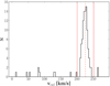 |
Fig. 3. Radial velocity distribution of our stars (black solid line). The dashed red line corresponds to the mean radial velocity from Battaglia et al. (2011) based on 174 probable members: vsys, helio = 226.0 ± 0.6 km s−1. The two solid red lines represent the ±3σ interval within which the membership zone is defined. |
The Sextans members were selected by requiring that their radial velocities fall within 3σ of the galaxy systemic velocity derived by Battaglia et al. (2011), 226.0 ± 0.6 km s−1, σ = 8.4 ± 0.4 km s−1. Twelve stars were identified as background or foreground interlopers; they are indicated as Non-member (v) in Table 2. Our final cleaned sample has a mean velocity and dispersion of vsys, helio = 224.9 ± 1.9 km s−1, σ = 7.7 ± 0.5 km s−1 in perfect agreement with Battaglia et al. (2011).
The dataset has been acquired over a time period of 1 month, and this time delay between the HR10 and HR13/HR14 spectra allowed us to look for binaries. These were identified based on radial velocities derived in each grism differing by more than 1σ, the error on the velocity. This corresponded to differences in velocities of Δvrad, HR between 7 and 35 km s−1. A total of 13 binary systems were identified in this way, for which the mean radial velocities in Table 2 are preceded by a tilde symbol. We also identified five carbon stars with a strong C2 band head. A preliminary analysis shows that these are CEMP-s stars. Further investigation of these stars is postponed to another paper.
Five stars (S05-72, S08-321, S08-111, S08-301, and S08-293) with overly poor-quality spectra and very unstable solutions for their abundances have also been removed from our investigation. These latter stars usually fall at the margins of the photometric RGB and are classified as Non-member (c) in Table 2. As a result of the above selection, our final sample encompasses 81 RGB Sextans stars.
4. Stellar atmosphere models
Our full sample is distributed along the Sextans RGB down to the horizontal branch level, that is, reaching uncommonly faint magnitudes for high-resolution spectroscopic analyses. For that reason, the elemental abundances of the GIRAFFE sample were derived by synthesis based on a χ2 minimisation procedure, which can balance the derivation of the chemical abundances over the widest possible wavelength range at once. This procedure is described in Sect. 7. Two stars were sufficiently bright to be fed to UVES. These have been analysed in a classical way, which is detailed in Sect. 6, based on the equivalent widths of their individual absorption lines.
In both cases, we adopted the MARCS 1D spherical atmosphere models, which were downloaded from the MARCS website2 (Gustafsson et al. 2008), and interpolated using the code of Thomas Masseron available on the same website. We assumed standard values of [α/Fe] following the Galactic disc and halo, namely +0.4 for [Fe/H] ≤ −1.5, +0.3 for [Fe/H] = −0.75, +0.2 for [Fe/H] = −0.54, +0.1 for [Fe/H] = −0.25, and +0.0 for [Fe/H] ≥ 0.0.
5. Photometric parameters
The photometric estimates of the stellar parameters Teff, log g, and vturb were based on the ESO 2.2m WFI V and I-band magnitudes (Tolstoy et al. 2004; Battaglia et al. 2006, 2011), as well as on the J, H, Ks WFCAM LAS UKIRT photometry calibrated onto the 2MASS photometric system (Skrutskie et al. 2006). These magnitudes are provided in Table 2.
For each star, the photometric effective temperature is taken as the simple average of the four colour temperatures TV − I, TV − J, TV − H, and TV − K obtained with the calibration of Ramírez & Meléndez (2005). When possible, the metallicity estimate from the CaT was used as initial iron abundance; otherwise we adopted the mean metallicity of the Sextans stellar population, [Fe/H] = −1.9, as given by Battaglia et al. (2011). We used EB − V = 0.0477 (Schlegel et al. 1998) and the reddening law, AV = 3.24 EB − V, of Cardelli et al. (1989). The stellar surface gravities were estimated from the stellar effective temperature and the bolometric correction calculated as in Alonso et al. (1999). We adopted a distance of 90 kpc (Tafelmeyer et al. 2010; Battaglia et al. 2011), a 0.8 M⊙ stellar mass for our sample stars and log g⊙ = 4.44, Teff⊙ = 5790 K, and MBol, ⊙ = 4.75. The micro-turbulence velocities were derived according to the empirical relation vturb = 2.0−0.2 × log g of Anthony-Twarog et al. (2013). The effective temperature for each colour, the bolometric corrections and initial metallicities are provided in Table 3.
These photometric parameters were the final ones for the GIRAFFE sample, while Teff and vturb could be further spectroscopically adjusted for the two stars observed with UVES as described in Sect. 6.
6. Analysis of the two stars observed with UVES
S05-5 and S08-229 were sufficiently bright to be allocated to two of the eight UVES fibres of the FLAMES configuration. These stars were analysed in the same way as in our previous publications on high-resolution spectroscopic studies in dwarf spheroidal galaxies (e.g. Letarte et al. 2006, 2010; Tafelmeyer et al. 2010; Jablonka et al. 2015; Hill et al. 2019). The abundance analysis has been performed using the local thermodynamical equilibrium (LTE) code CALRAI first developed by Spite (1967) (see also Cayrel et al. 1991 for the atomic part), and continuously updated over the years. We summarise the main steps below.
6.1. Measurements
The absorption features were measured following the line list of Tafelmeyer et al. (2010) which combines those of Letarte et al. (2010) and Cayrel et al. (2004). The equivalent widths were measured with DAOSPEC. As DAOSPEC fits absorption lines with Gaussians that have a fixed FWHM, the equivalent widths of strong lines with prominent wings are systematically underestimated. Therefore, lines with equivalent widths larger than 180 mÅ were discarded. Table 5 lists the lines and their equivalent widths. The present analysis focuses on the elements derived in the HR10, HR13, and HR14 grisms. A discussion of the other elements accessible thanks to the UVES wavelength coverage and high resolution is deffered to a forthcoming paper.
6.2. Final atmospheric parameters and error estimates
The convergence to our final effective temperatures and the microturbulence velocities (vturb) presented in Table 6 was achieved iteratively, as a trade off between minimising the trends of metallicity derived from the Fe I lines with excitation potentials and equivalent widths on the one hand and minimising the difference between photometric and spectroscopic temperatures on the other hand. Starting from the initial photometric parameters we adjusted Teff and vturb allowing for deviation by no more than 2 σ (the uncertainty) of the slopes. This yielded new metallicities which were then fed back into the photometric calibration to get new photometric temperatures and gravities. No more than two or three iterations were needed to converge to our final atmospheric parameters.
The predicted equivalent widths rather than the observed ones were considered in this procedure, because the errors on the measurements can bias the slope of the diagnostic plots (see Magain 1984). However, the surface gravities were kept fixed to their photometric values due to the small number of Fe II lines and possible NLTE effects, which might affect the ionisation equilibrium.
The final abundances are calculated as the weighted mean of the abundances obtained from the individual lines, where the weights are the inverse variances of the single line abundances. These variances were propagated by CALRAI from the estimated errors on the corresponding equivalent widths. They are listed in Table 7. Table 8 provides the errors on the abundances linked to the uncertainties on atmospheric parameters for the two stars observed with UVES.
Abundances for S05-5, S08-229 observed with UVES.
Errors due to uncertainties in atmospheric parameters for S05-5, S08-229 observed with UVES.
7. Analysis of the GIRAFFE sample
7.1. Synthetic grid
[Fe/H]. To determine [Fe/H], a library of synthetic spectra covering the HR10, HR13, and HR14 wavelength regions was created with MOOG3 (August 2010 Version). The stellar spectra were generated at the resolution R = 40 000, over 4200 K ≤ Teff ≤ 5300 K with a step of 50 K, 0.5 ≤ log g ≤ 2.5 with a step of 0.1 dex, 1.4 ≤ vturb ≤ 2.0 with a step of 0.2 km s−1, and −4.0 ≤ [Fe/H] ≤ −0.5 with a step of 0.1 dex.
Elemental abundances. To derive the other elemental abundances, [X/H], we created two sets of synthetic spectra at given Teff, log g, vturb, and [Fe/H]. The first set of synthetic spectra covered an interval of 6 dex in [X/H], from [X/H] = −5.0 to [X/H] = 1.0, in 0.5 dex steps. The second set covered only 2 dex in [X/H] but with steps of 0.05 dex and was centred on the first estimated [X/H] of the star under analysis.
The resolution of the synthetic spectra was adjusted to those of the observed spectra, i.e. to resolving powers R = 19 800 for HR10, 22 500 for HR13, and 17 740 for HR14, by convolution with Gaussians with FWHM = 15.2, 13.3, and 16.9 km s−1, and was then normalised with MOOG. A number of different macroscopic mechanisms can broaden the stellar absorption features. The dominant one in our case is the instrumental broadening. However, as is often the case, applying this instrumental broadening to theoretical spectra is insufficient. Macro-turbulence and possible rotation need to be taken into account. These corrections were estimated on the four brightest stars of the GIRAFFE sample for which both a classical analysis based on line equivalent widths and the spectral synthesis could be independently performed (see Sect. 8.2). For this particular purpose, we only considered the Fe I lines. We found that an additional broadening by σ = 9.0 km s−1, 7.9 km s−1 and 7.6 km s−1 Gaussians for the HR10, HR13, and HR14 gratings, respectively, resulted in the best agreement in metallicities between the two types of analyses. These broadenings were therefore applied to the synthetic spectra for the three respective setups.
7.2. Synthesis principles
The elemental abundances of the GIRAFFE sample stars were derived by synthesis based on a χ2 minimisation procedure, in which
 (1)
(1)
where i is the pixel index and y the normalized flux of this pixel in the observed yobs, i spectrum as well as in the model synthetic ymod, i one.
For each chemical species, a global χ2 was calculated for all detected lines. The match between the synthetic and observed spectra was estimated in windows centred on the lines with widths of 22 pixels in HR10 and HR13 (1.05 Å), and 28 pixels (1.35 Å) in HR14. The width of these windows were calculated as 1.75 × FWHM, with FWHM being the spectral resolution of the grating under consideration.
The final χ2 value was summed over the lines in the three wavelength bands:
 (2)
(2)
7.3. Iron abundance
Starting from the Fe I line list of Tafelmeyer et al. (2010), we discarded the weakest lines which would be overly altered by the noise or blended. This selection ensures that our sample stars, spanning a large portion of the RGB, are all analysed in a homogeneous way. Our final line list is presented in Table 9. It encompasses 50 Fe I lines: 20 in HR10, 21 in HR13, and 9 in HR14. The HR13 and HR14 grisms have a small overlapping region. The lines in common were considered in the HR13 part only, taking advantage of its higher resolution.
For each star of photometric Teff, log g, and vturb, we selected the closest synthetic spectra with these parameters, namely with Teff within 50 K and log g within 0.1 dex. We interpolated them at the value of vturb. The χ2 values were then calculated for [Fe/H] varying from −4.0 to −0.5 in steps of 0.1 dex. Finally, the χ2–[Fe/H] relation was interpolated to a 0.01 dex step level in order to properly locate the minimum of the relation. The corresponding metallicities are given in Table 6.
We note that the maximum differences in Teff and log g between the photometric stellar parameters and the values adopted in the grid are 25 K and 0.05 dex, respectively. These differences are smaller than the systematic errors on the photometric estimates.
Re-inserting the final value of [Fe/H] into the colour–temperature formula does not significantly affect the effective temperatures. The maximum difference ΔTeff with respect to the initial estimate is 45 K, which is twice smaller than the systematic errors. Therefore, we kept the initial effective photometric temperatures.
7.4. Elemental abundances
Once [Fe/H] was determined, we derived the abundances of the rest of the elements using the same chi-squared minimisation procedure as for the metallicity. Again, the χ2–[X/H] relation was interpolated to reach a [X/H] step of 0.01 dex. Thanks to the wavelength coverage of our spectra we were able to derive abundances of ten elements: Mg, Ca, Sc, Ti, Cr, Mn, Co, Ni, Ba, and Eu.
We took into account the hyperfine structure for the odd atomic number isotopes: Sc II (Prochaska et al. 2000), Mn I (from Kurucz database4 as in North et al. 2012), Co I (Prochaska et al. 2000), Ba II (Prochaska et al. 2000), and Eu II (Lawler et al. 2001 as in Van der Swaelmen et al. 2013). The complete line list with wavelengths, excitation potentials, oscillator strengths, and C6 constants is presented in Table 9. The hyperfine components are indicated in italics and their corresponding lines are followed by the text (“equi”). The abundances are given in Tables 10–12. The solar abundances from Grevesse & Sauval (1998) are repeated in the first line of these three tables. Figure 4 presents three examples of observed and synthetic best fits that span the range of S/N encountered in this study.
 |
Fig. 4. Part of the HR10 spectrum of S08-6 (top), S08-242 (middle) and S05-67 (bottom) in black with their synthetic best fits over-plotted in red. A set of lines used in abundance determination are indicated for each star. The stars are ranked from top to bottom by decreasing signal-to-noise ratios: 83, 38, and 23. |
7.5. Error budget
The errors on the abundances derived for the GIRAFFE sample, reported as error bars in all figures, correspond to the quadratic sum of the systematic errors and the random errors defined below and indicated in Tables 10–12.
Systematic errors. Taking as systematic errors a typical variation of ±100 K in effective temperatures, which accurately represents (75% of our sample) the maximum variation in Teff from one colour to the other, we re-derived the stellar parameters and abundances for each star. We obtained small systematic shifts: between 0.04 and 0.075 for the surface gravities, and an average of 0.01 km s−1 on the micro-turbulence velocities. The systematic errors on [Fe/H] range from 0.1 to 0.17 dex, with an increasing trend with decreasing effective temperature. For the other abundances, the smaller systematic errors are found for Mg, Sc, Ti, and Eu with 0.05 dex on average and the larger for Cr and Mn with 0.2 dex on average. Examples are provided in Fig. 5.
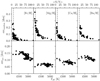 |
Fig. 5. Distribution of the systematic and random errors as a function of S/N and effective temperature. These examples are shown for the elements for which we have the largest number of detections. We refer to the main text for a detailed definition of these errors. |
We also considered the effect of the uncertainty on the distance of Sextans, which is ∼±5 kpc around our adopted value (Irwin et al. 1990; Lee et al. 2003). This translates into an uncertainty of 0.05 dex on the surface gravities, and corresponds to the same order of magnitude as varying the effective temperatures by ±100 K.
Random errors. Variations in S/Ns may well impact the results differently depending on the atmospheric parameters and the chemical enrichment of the stars. Our sample spans more than 1 dex in [Fe/H] and 1000 K in Teff.
The random errors on the abundances were therefore estimated from Monte Carlo simulations. For each star, at given Teff, log g, vturb, and [Fe/H], we generated 1000 spectra with the same S/N as the observed spectrum. The abundances were then determined on these simulated noisy spectra. The adopted random error corresponds to the standard deviation of the Gaussian function that best fits the distribution of the 1000 obtained abundances. Figure 5 presents some example of these randoms errors on [Fe/H] and [X/H] as a function of S/N. From one set to the another, the higher the effective temperature and surface gravity, the larger the impact of the noise, because the lines are smaller.
Based on this exercise, we only considered the abundances of stars for which we have spectra of S/N > 10 as secure. Indeed, regardless of the reliability of the metallicities, the errors on the other elements can reach 1 dex, hampering any reliable interpretation.
8. How well do we perform?
The purpose of this section is to assess the quality of our analysis and also to check that previously published stellar abundances in Sextans can be combined with our work to provide a robust view of Sextans’ chemical evolution.
8.1. Comparison with the medium-resolution CaT sample
Calcium triplet metallicity estimates are available for a subset of 32 stars with S/N > 10 (Battaglia et al. 2011). Figure 6 presents a comparison between the [Fe/H] estimates of this latter study and ours. The agreement is excellent with a mean difference of 0.0014 dex and a standard deviation of 0.137 dex. This comparison led us to discard from further analysis two stars with Δ[Fe/H] > 0.4 dex common to both studies: S08-75 and S08-59, identified with triangles in Fig. 6. A closer look indeed reveals that the metallicity of S08-75 is based on only nine iron lines because its spectra have been polluted by simultaneous calibration fibres in HR10 and HR13. The position of S08-59 on the CMD of Sextans sheds doubt on its RGB status; it is most likely a horizontal branch star.
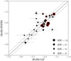 |
Fig. 6. Comparison between the CaT metallicity estimates and the [Fe/H] values derived from spectral synthesis (SYNTH). The size of the points is a function of the S/N of the spectra. The two stars S08-75 and S08-59, which have been discarded from further analysis (see text) are identified with triangles. We highlight in red the stars which have been independently analysed with a classical method based on equivalent widths and which are in Fig. 7. |
8.2. Equivalent width versus synthesis
Given that the chemical abundances in the literature are generally derived with methods based on equivalent widths, but also, and more specific to this work, because two of our sample stars were gathered with UVES and analysed in this classical way, it is important to check for the existence of any significant bias between this type of analysis and the spectral synthesis (“SYNTH”).
To this aim, a subsample of 11 bright (V < 19 mag) stars (S08-3, S08-6, S05-10, S08-38, S08-239, S08-241, S08-242, S07-69, S05-60, S08-246, and S08-183) from the GIRAFFE sample was independently analysed with CALRAI in the same way as our two UVES stars. We refer to this method as “EQW” in the following. The only difference with the analysis of the UVES stars is that we fixed Teff to its photometric value. Only the turbulence velocity vturb was determined by requesting a null slope (within the fit uncertainties resulting from the measurement errors) of the relation between the abundances and equivalent widths of the individual Fe I lines. The line list and equivalent widths are provided in Table 13.
Figure 7 summarises the comparison between the two methods, EQW and SYNTH, for the determination of Fe I. The sizes of the symbols are proportional to the spectrum average S/Ns. The dashed lines are placed at ±0.1 dex of the x = y line. There is a tendency for the EQW Fe I abundances to be slightly higher – by ∼0.08 dex on average, with a standard deviation of 0.09 dex – than the SYNTH metallicities.
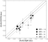 |
Fig. 7. Comparison between the metallicity derived from our synthesis code, [Fe/H]SYNTH, and with a classical method based on the equivalent widths of the individual iron lines Fe/H]EQW (see text). The solid line traces the line of equality while the dashed lines indicate a variation by ±0.1 dex. The size of the black circles increases with the S/N of the spectra. |
Even if this difference falls well within the error bars, it is interesting to try and understand its origin. Different factors can be invoked and they are sometimes combined: a variety of S/Ns, the use of different line lists, and different ways of deriving the micro-turbulence velocities between the two techniques (requesting a null slope comparing Fe I abundances and equivalents widths for EQW, while it is estimated from an empirical relation linked to log g for SYNTH). To illustrate this latter point, the relation between the differences in [Fe/H] and the variations in vturb is shown in Fig. 8: a difference in vturb of 0.1 km s−1 can result in a Δ[Fe/H] ≥ 0.1 dex. The star S05-60 has the largest metallicity difference between EQW and SYNTH. As a matter of fact, the micro-turbulence velocities differ by 0.3 km s−1 between the two methods.
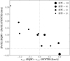 |
Fig. 8. Differences between the metallicities obtained by the EQW and SYNTH methods as a function of the differences of the stellar micro-turbulence velocities. |
The case of the star S08-6 illustrates the influence of the linelist. The difference of 0.1 dex between the EQW and SYNTH results, [Fe/H]EQW = −1.5 and [Fe/H]SYNTH = −1.6, is reduced to 0.03 dex simply by using the exact same Fe I line list. In this case, [Fe/H]SYNTH = −1.53 dex.
Figure 9 provides a comparison of the two techniques for three α-elements Mg, Ca, and Ti II. These are the elements for which we have the largest number of detections, providing a reliable comparison. Here, again the abundances resulting from the two techniques are perfectly consistent within the error bars.
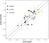 |
Fig. 9. Comparison between the abundances of three α-elements derived by the EQW and SYNTH methods. The solid line traces the line of equality while the dashed lines indicate a variation by ±0.1 dex around this line. |
8.3. Comparison with literature
S08-3 is the brightest star of the GIRAFFE sample. It has also been observed with HIRES at the Keck I telescope at a resolution of R ∼ 34 000 and analysed by Shetrone et al. (2001). There are ten elements in common between the three independent types of analyses, SYNTH, EQW in this work, and Shetrone et al. (2001). Figure 10 presents a comparison of the results from these analyses. The median of the difference between the studies is 0.09 dex with a minimum at 0.01 dex and a maximum at 0.30 dex, all well within the error bars.
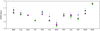 |
Fig. 10. Elemental abundances of the star S08-3. The green circles refer to this study, the blue stars come from Shetrone et al. (2001), and the magenta squares are from the EQW analysis. |
In conclusion, the tests we performed confirm that the choice of one or the other technique to derive the elemental abundances is a source of only minor variation in the results, and we did not find any bias or deviation that would exceed the uncertainties on the abundances. Therefore, we confidently combine our UVES/EQW and GIRAFFE/SYNTH analyses with previously published results in following discussion.
9. Results
9.1. Metallicity distribution function
The metallicity distribution function of our FLAMES sample stars is presented in Fig. 11. The Sextans members (green solid line) are compared to the DART medium-resolution Ca triplet survey (blue solid line; Battaglia et al. 2011). Our distribution peaks around [Fe/H] = −1.8 dex and is almost completely included in the CaT distribution. Keeping only the stars with CaT metallicity estimates, we obtain the filled green area peaking at the same [Fe/H] value as the original CaT distribution. Our full dataset is on average slightly more metal-rich than the full CaT DART survey. This is most likely a consequence of the different spatial distribution of the two samples (see Fig. 1) and the presence of a radial gradient in Sextans (Lee et al. 2009; Battaglia et al. 2011). Our field is centrally concentrated (diameter of 25′), while the DART CaT survey covers FLAMES fields distributed from the centre to near the tidal radius of Sextans. Revaz & Jablonka (2018) have shown that gas tend to concentrate in the central regions of the dwarf spheroidal galaxies which consequently have the longest star formation activity. Indeed the analysis of the colour-magnitude diagrams indicates progressively longer timescales of star formation towards the galaxy centre (Lee et al. 2009). Therefore, our central FLAMES field is probing the full chemical evolution of Sextans as illustrated by the fact that we cover a very large metallicity range, from −3.2 to −1.5 dex.
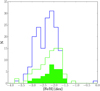 |
Fig. 11. Metallicity distribution function of the Sextans stars. Following the same colour code as in Figs. 1 and 2. The blue solid line corresponds to the probable members of the CaT DART sample (Battaglia et al. 2011), while the green solid line shows our high-resolution sample. The filled green area corresponds to the subsample of our members previously studied in CaT. |
Among the stars with S/N ≥ 10 spectra, two are found at [Fe/H] ≤ −3: S05-94 and S08-257. Two more have [Fe/H] ∼ −2.90, namely S08-71 and S11-97, which makes them eligible, within the uncertainties, for membership of the class of extremely metal-poor stars. Indeed, S11-97 has been reobserved with UVES at a resolution of ∼40 000 and is confirmed as an EMP (Lucchesi et al., in prep.).
9.2. α-elements
Three α-elements are accessible in our wavelength range: Mg I (1 line), Ca I (13 lines), and Ti at its two ionization levels, Ti I (4 lines) and Ti II (4 lines). The distribution of [α/Fe] as a function of [Fe/H] is presented in Fig. 12 for Sextans and the Milky Way stars. Only stars with S/N > 10 spectra are considered. Our study significantly increases the existing samples at high resolution with 46 new stars in [Mg/Fe], 37 in [Ca/Fe], and 34 in [Ti/Fe].
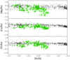 |
Fig. 12. Distribution of [Mg/Fe], [Ca/Fe], and [Ti/Fe] as a function of [Fe/H] for the Sextans dSph (in green). The circles are the new stars from our Giraffe sample; the squares display the re-analysed sample of Shetrone et al. (2003); the stellar symbols stand for the dataset of Aoki et al. (2009), the down-pointing triangles for Kirby et al. (2010), the right-pointing triangles for Tafelmeyer et al. (2010), and the diamond from Honda et al. (2011). The Milky Way comparison sample shown in grey encompasses Venn et al. (2004), Cayrel et al. (2004), François et al. (2007), Gratton et al. (2003), Cohen et al. (2006, 2008, 2013), Honda et al. (2004), Reddy et al. (2006), Yong et al. (2013), Lai et al. (2007), Spite et al. (2005), Aoki et al. (2005, 2007), Barklem et al. (2005), Ishigaki et al. (2013). |
The comparison samples taken from the literature come from works conducted at high spectroscopic resolution, at the exception of Kirby et al. (2010) with R ∼ 7000. In order to keep the level of accuracy in abundance ratios as homogeneous as possible between the different references, we restricted the sample of Kirby et al. (2010) to the eight stars with error on [Fe/H] ≤ 0.12 dex. The star S15-19 was analysed by both Aoki et al. (2009) and Honda et al. (2011). We consider the abundances of the latter study. We refer the reader to Lucchesi et al. (in prep.) for a full reanalysis of the sample of Aoki et al. (2009).
9.2.1. Ti I versus Ti II
Due to the weakness of the Ti I lines, we were only able to derive the [Ti I/Fe] abundance ratio in four stars (S05-47, S08-3, S08-6, S08-38), while [Ti II/Fe] could be calculated in 32 stars. Still, the result on [Ti I/Fe] for S05-47 is extremely uncertain as it relies on a single line. The three other stars show lower [Ti I/Fe] than [Ti II/Fe] but the estimates agree within the error bars. In the following, [Ti/Fe] is taken as [Ti II/Fe] similarly to our previous studies.
9.2.2. Comparison between α-elements and impact of the SNeIa
Figure 12 shows the common trend between the three α-elements and [Fe/H]: a plateau at constant [α/Fe] with [Fe/H] followed by a decrease down to subsolar values. The scatter in abundance ratios scales with the number of lines of each element usable in the analysis and the S/N of the spectra. This is particularly true for [Mg/Fe], for which the scatter at fixed [Fe/H] and the error bars are the largest. Regarding the stars with subsolar [Mg/Fe] values, three are particularly noticeable, S08-282, S08-280, and S05-47, in order of increasing [Fe/H], with [Mg/Fe] < −0.5. While the exact Mg abundance for these stars is not yet secure, as uncertainties are large, the comparison with other stars in the sample at similar atmospheric parameters confirms their low values: S08-282 (Teff = 5044 K, log g = 1.96, 1.61, [Fe/H] = −1.96) was compared to S05-84 (5048 K, 1.92, 1.62, −1.96; [Mg/Fe] = 0.5), and S05-47 (4654 K, 1.28, 1.74, −1.64) to S08-242 (4657 K, 1.44, 1.44, −1.71; [Mg/Fe] = +0.05).
The trend seen in Fig. 12 is formed by a plateau at [α/Fe] ∼ 0.4 ended by the so-called knee, which is the [Fe/H] origin of the decrease in [α/Fe] with increasing metallicity, corresponding to the time when, after a decrease in the galaxy star formation rate, the contribution of the SNeIa starts to dominate the chemical composition of the ISM. This new FLAMES sample offers for the first time a large number of stars with abundances derived at sufficient accuracy to estimate the location of this knee in Sextans at [Fe/H] ∼ −2 dex.
The galaxy star formation history shapes the morphology of the [α/Fe] versus [Fe/H] diagram. The similar position of the knee reveals similar star formation efficiency in the first few gigayears of the galaxy evolution, while the slope of the decrease in [α/Fe] is determined by the balance between the mass of metals ejected by the SNeIa on the one hand and by the SNeII on the other hand. Therefore, past the peak of its star formation rate, a system with extended star formation history will lead to a decrease in [α/Fe] versus [Fe/H] with a smaller slope than a galaxy that is quenched sharply. As a consequence, it is quite informative to compare the decreasing [α/Fe] branches of the classical dwarfs.
The position of the knee in the Carina dSph is still an open issue, most probably because of the overlap of stellar populations coming from the three different star formation episodes. It was tentatively detected between −2.7 and −2.3 dex (Lemasle et al. 2012; Venn et al. 2012), however not confirmed by Norris et al. (2017). The spectroscopic samples of other dSphs, such as those of Draco and Ursa Minor, are still too small to robustly locate their knees (Cohen & Huang 2009, 2010). The Fornax and Sculptor dSphs, for which there exists sufficiently large spectroscopic samples, are therefore the two systems that are comparable to Sextans (Letarte et al. 2010; Hill et al. 2019). The Sextans and Sculptor dSphs have formed stars for 4 to 6 Gyr, respectively (Lee et al. 2009; de Boer et al. 2011), while the period of star formation in Fornax is more extended, beyond 12 Gyr even if at a low final rate (de Boer et al. 2012). Figure 13 compares the corresponding [α/Fe] versus [Fe/H] patterns, and provides a detailed view of the knee region. Formally, the position of the Sextans knee is slightly below those of Sculptor (∼ − 1.8 Tolstoy et al. 2009), and Fornax (∼ − 1.9 Hendricks et al. 2014). In practice these values are essentially identical given the uncertainty on both [Fe/H] and on the exact position of the knee due to the scatter in [α/Fe] at fixed metallicity. This is an impressive agreement given that these galaxies span a factor of ∼50 in final stellar masses and a range of dynamical status (Sculptor 2.3 × 10⁶M⋆ (σ = 9.2 km s−1), Sextans 0.44 × 10⁶M⋆ (σ = 7.9 km s−1), Fornax 20 × 106M⋆ (σ = 11.7 km s−1); McConnachie 2012). It provides evidence that, in the first gigayears, the star formation efficiency (the mass of newly born stars per unit gas mass) of the three galaxies was very similar. This period of time corresponds to the initial merging sequence of small galactic units building the galaxy potential well, which will then be massive enough (or not) to resist the UV-background heating (Revaz & Jablonka 2018). In other words, up to the knee, the star formation processes are essentially dominated by the smaller building blocks. The chemical evolution past the knee then reflects the in-situ star formation when the mass of the systems is already in place. This part depends on the degree to which the galaxies have been impacted (quenched) by the UV background. As expected from the length of their star formation histories, the slope of the [α/Fe] versus [Fe/H] branches is steeper for Sextans than for Sculptor and Fornax.
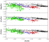 |
Fig. 13. Comparison between the three classical dwarfs, Sextans (green), Sculptor (blue), and Fornax (red), and the Milky Way (grey) in the region of the knee in [α/Fe]. |
9.3. Iron-peak elements
The number of stars for which the abundances could be determined is smaller than for the α elements: 20 stars for Cr, 5 stars for Mn, 2 stars for Co, and 6 stars for Ni, as a consequence of the weakness of the lines and the large differences in the S/Ns of the spectra.
Figure 14 presents the abundance ratios of Sc, Ni, and Co to Fe. These have been derived from three lines of Sc II, 6 lines of Ni I, and one line of Co I. The production of Sc is dominated by SNeII (Woosley et al. 2002; Battistini & Bensby 2015), and therefore, as expected, [Sc/Fe] follows the same trend with [Fe/H] as the α-elements. The case of Ni and Co is different because these elements can also be largely produced by SNeIa (Timmes et al. 2003; Travaglio et al. 2005). The ∼2 Gyr of star formation history of Sextans, albeit with a sharp drop in SFR beyond the explosion timescale of SNeIa, makes it an ideal system to witness their nucleosynthesis imprint. Kirby et al. (2019) conducted an analysis of the Cr, Ni, and Co abundance trends in dwarf spheroidals in order to constrain the nature of the SNeIa progenitors. In particular, they compared the theoretical yields of Chandrasekhar-mass SNIa and sub-Chandrasekhar-mass models to existing observed abundances in dwarf galaxies. Figure 14 confirms the decline of [Co/Fe] and [Ni/Fe] past [Fe/H] ≥ −2. This implies that the production of Ni and Co is lower than the yield of Fe in SNeIa. Our conclusions agree with those of Kirby et al. (2019), in that while the observation of [Co/Fe] is compatible with most of the models, the decrease in [Ni/Fe] down to subsolar values favours the explosion of double degenerate sub-Chandrasekhar-mass white dwarfs (Shen et al. 2018; Bravo et al. 2019). This nevertheless requires conformation with NLTE calculations when they become available.
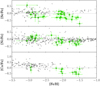 |
Fig. 14. Abundance ratio for the iron-peak elements Sc, Ni, and Sc for the Sextans dSph in green in comparison with the Milky-Way population in grey. Symbols are as in Fig. 12. |
Figure 15 shows the two other iron-peak elements that we were able to measure, Cr I (3 lines) and Mn I (4 lines). North et al. (2012) derived the abundance of Mn for the same stars as the present analysis. The results of their study agree with ours within 1σ uncertainties. Therefore, for the sake of homogeneity Fig. 15 displays the results of the synthetic approach of this work.
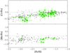 |
Fig. 15. Distribution of [Cr/Fe] (top panel) and [Mn/Fe] (bottom panel) for stars in Sextans and the Milky Way. Symbols are as in Fig. 12. |
Both Cr and Mn closely follow the Milky Way trends. There are no NLTE calculations available for the range of stellar atmospheric parameters covered by our sample, either for Cr or for Mn. Nevertheless, Bergemann & Cescutti (2010) show that the steady increase of [Cr/Fe] with metallicity observed for the MW metal-poor stars is an artefact of neglecting NLTE effects in the line formation of Cr. These NLTE corrections are positive and move [Cr/Fe] close the solar value over the full range of metallicities. Given the similar behaviour of the metal-poor population in dwarfs and the Milky Way, there are good reasons to believe that NLTE is also at the origin of the low [Cr/Fe] values at [Fe/H] ≤ −2. The fact that [Cr/Fe] is again solar beyond the position of the knee in Sextans suggests that the production of chromium is very similar in SNeII and SNeIa.
Departures from LTE have been studied by Bergemann & Gehren (2008) and Bergemann et al. (2019) for slightly hotter stars than our sample and for different lines from those in our list but in the same metallicity range. The NLTE abundances of Mn were systematically higher than the LTE abundances by up to 0.6 dex. This is probably more than needed for our sample in Sextans to place the sequence of [Mn/Fe] on the solar sequence. if confirmed, similarly to Cr, the production of Mn should be very similar in SNeII and SNeIa.
9.4. Neutron-capture elements
We were able to analyse two neutron-capture process elements: Ba II (2 lines) measured for 39 stars and Eu II (1 line) obtained for 7 stars. These elements are produced in the rapid (r-) and the slow (s-) neutron capture processes.
Figure 16 presents the evolution of [Ba/Fe], [Eu/Fe], and [Ba/Eu] as a function of [Fe/H]. The Sextans stars follow the trend of the MW stars in [Ba/Fe], with a plateau very slightly above the solar level following the ∼1 dex initial scatter between [Fe/H] ∼ −3 and [Fe/H] ∼ −2.5. We were only able to measure europium for a few stars. These sample the solar plateau in barium. There is a small but clear decrease of [Eu/Fe] at [Fe/H] ≥ −2, indicating that the production of iron progressively overtakes that of Eu, as expected from the decrease in star formation rate and the growing impact of the explosions of SNeIa. There is a slight increasing trend of [Ba/Eu] with [Fe/H], inversely reflecting the variation of [Eu/Fe] with [Fe/H], with all values [Ba/Eu] below [Fe/H] ∼ −1.5 being subsolar indicating that below [Fe/H] ∼ −2, barium is produced either entirely or mainly by the r-process. The low-metallicity asymptotic giant branch stars (AGBs) are sufficiently numerous at [Fe/H] ≥ −2 that [Ba/Eu] increases by the addition of the s-process elements. Sextans’s chemical evolution does not extend as far as that of Sculptor; in particular, there is no star in the −1.5 to −1 [Fe/H] range. However, between [Fe/H] = −2.3 and −1.5 the two galaxies share the same chemical trends, implying similar fractions of SNeIa and low-metallicity AGBs (Hill et al. 2019). The comparison with Fornax is more difficult due to the lack of measurements of europium. Nevertheless, in the same low-metallicity range, Fornax does show the same plateau at [Ba/Fe] ∼ 0, confirming the universal timescale of the onset and rise of the s-process (Lemasle et al. 2014).
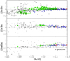 |
Fig. 16. Distributions of [Ba/Fe] (top panel), [Eu/Fe] (middle panel), and [Ba/Eu] (bottom panel) for stars in Sextans (green), Fornax (red), Sculptor (blue), and the Milky Way (grey). The upper limit on Eu of Honda et al. (2011) for S15-19 at [Fe/H] ∼ −3 is indicated with an arrow. |
10. Summary and conclusions
We present an analysis of the FLAMES dataset, targeting the central 25′ region of the Sextans dSph. This dataset is the third part of the ESO large program 171.B-0588(A) obtained by the Dwarf galaxy Abundances and Radial-velocities Team (DART) together with the Fornax and Sculptor galaxies (Letarte et al. 2010; Hill et al. 2019). A total of 101 stars have been gathered with the HR10, HR13, and H14 gratings of the multi-fibre spectrograph FLAMES/GIRAFFE. Two fibres were linked to the red arm of the UVES spectrograph.
Our sample is composed of RGB stars down to V ∼ 20.5 mag, the level of the horizontal branch in Sextans. Spectra in the CaT region are also available for some of them (Battaglia et al. 2011), with first estimates of their metallicity. The rest of the sample was photometrically selected as corresponding to the position of Sextans in the V, I colour-magnitude diagram. We provide [Fe/H] determination for 81 stars, which cover the wide metallicity range [Fe/H] = −3.2 to −1.5 dex. After a thorough investigation of the random and systematic errors, we deliver accurate abundances of three α-elements (Mg, Ca and Ti), five iron-peak elements (Sc, Cr, Mn, Co, and Ni), and two neutron-capture elements (Ba and Eu). Despite the small stellar mass of Sextans, its stellar population reveals a rich chemical evolution involving core collapse and Type Ia supernovae, as well as low metallicity AGBs.
The analysis of the α-elements reveals a plateau at [α/Fe] ∼ 0.4 followed by decrease, corresponding to the time when the contribution of the SNeIa begins to dominate the chemical composition of the ISM. This new FLAMES sample offers for the first time a large number of stars with abundances derived at sufficient accuracy to estimate the location of the knee in Sextans at [Fe/H] ∼ −2 dex, very close to both the Sculptor and Fornax dSphs, despite their very different masses and star formation histories. This provides evidence that, in the first gigayears, the star formation of the three galaxies followed similar processes, such as the accretion of smaller building-blocks before the period of reionisation.
[Sc/Fe] follows the same trend with [Fe/H] as the α-elements, confirming that its production is dominated by SNeII. Ni and Co can be produced by SNeII and SNeIa. We confirm the decline of [Co/Fe] and [Ni/Fe] past [Fe/H] ≥ −2, implying that the production of Ni and Co in SNeIa is lower than that of Fe. While the observation of [Co/Fe] is compatible with most of the models of SNeIa, the decrease in [Ni/Fe] favours the explosion of double degenerate sub-Chandrasekhar-mass white dwarfs. The fact that [Cr/Fe] is solar and [Mn/Fe] is flat beyond the position of the knee in Sextans suggests that the production of chromium and manganese is very similar in SNeII and SNeIa.
The stellar population of Sextans follows the same trend as the Milky Way stars in [Ba/Fe], with a plateau at solar level following the initial scatter below [Fe/H] ∼ −3. The trend of [Ba/Eu] with [Fe/H] indicates that below [Fe/H] ∼ −2, barium is produced either entirely or at least principally by the rapid neutron capture channel. The low- metallicity AGBs are sufficiently numerous at [Fe/H] ∼ −2 that [Ba/Eu] increases by the addition of the s-process elements. In the metallicity region covered by the three galaxies, Sculptor, Fornax, and Sextans share the same trends, suggesting similar fractions of SNeIa and low-metallicity AGBs in their early evolution.
DAOSPEC has been written by P. B. Stetson for the Dominion Astrophysical Observatory of the Herzberg Institute of Astrophysics, National Research Council, Canada.
MOOG (Sneden 1973) is a FORTRAN code designed to perform a variety of LTE line analyses and spectrum synthesis with the aim being to help with determination of the stellar chemical composition. The basic equations of the stellar line analysis in LTE are used following the formulation of Edmonds (1969). Much of the MOOG code follows in a general way the WIDTH and SYNTHE codes of R. L. Kurucz (http://kurucz.harvard.edu/).
Available at http://kurucz.harvard.edu/linelists.html
Acknowledgments
The authors are indebted to the International Space Science Institute (ISSI), Bern, Switzerland, for supporting and funding the international teams “First stars in dwarf galaxies” and “Pristine”. RT, PJ, PN, and CL also thank the Swiss National Science Foundation for its support.
References
- Alonso, A., Arribas, S., & Martínez-Roger, C. 1999, A&AS, 140, 261 [NASA ADS] [CrossRef] [EDP Sciences] [Google Scholar]
- Anthony-Twarog, B. J., Deliyannis, C. P., Rich, E., & Twarog, B. A. 2013, ApJ, 767, L19 [NASA ADS] [CrossRef] [Google Scholar]
- Aoki, W., Honda, S., Beers, T. C., et al. 2005, ApJ, 632, 611 [NASA ADS] [CrossRef] [Google Scholar]
- Aoki, W., Beers, T. C., Christlieb, N., et al. 2007, ApJ, 655, 492 [NASA ADS] [CrossRef] [Google Scholar]
- Aoki, W., Arimoto, N., Sadakane, K., et al. 2009, A&A, 502, 569 [NASA ADS] [CrossRef] [EDP Sciences] [Google Scholar]
- Barklem, P. S., Christlieb, N., Beers, T. C., et al. 2005, A&A, 439, 129 [NASA ADS] [CrossRef] [EDP Sciences] [Google Scholar]
- Battaglia, G., Tolstoy, E., Helmi, A., et al. 2006, A&A, 459, 423 [NASA ADS] [CrossRef] [EDP Sciences] [Google Scholar]
- Battaglia, G., Tolstoy, E., Helmi, A., et al. 2011, MNRAS, 411, 1013 [NASA ADS] [CrossRef] [MathSciNet] [Google Scholar]
- Battistini, C., & Bensby, T. 2015, A&A, 577, A9 [NASA ADS] [CrossRef] [EDP Sciences] [Google Scholar]
- Bergemann, M., & Cescutti, G. 2010, A&A, 522, A9 [NASA ADS] [CrossRef] [EDP Sciences] [Google Scholar]
- Bergemann, M., & Gehren, T. 2008, A&A, 492, 823 [NASA ADS] [CrossRef] [EDP Sciences] [Google Scholar]
- Bergemann, M., Gallagher, A. J., Eitner, P., et al. 2019, A&A, 631, A80 [NASA ADS] [CrossRef] [EDP Sciences] [Google Scholar]
- Bravo, E., Badenes, C., & Martínez-Rodríguez, H. 2019, MNRAS, 482, 4346 [NASA ADS] [CrossRef] [Google Scholar]
- Cardelli, J. A., Clayton, G. C., & Mathis, J. S. 1989, ApJ, 345, 245 [NASA ADS] [CrossRef] [Google Scholar]
- Casetti-Dinescu, D. I., Girard, T. M., & Schriefer, M. 2018, MNRAS, 473, 4064 [NASA ADS] [CrossRef] [Google Scholar]
- Cayrel, R., Perrin, M.-N., Barbuy, B., & Buser, R. 1991, A&A, 247, 108 [Google Scholar]
- Cayrel, R., Depagne, E., Spite, M., et al. 2004, A&A, 416, 1117 [NASA ADS] [CrossRef] [EDP Sciences] [Google Scholar]
- Cicuéndez, L., & Battaglia, G. 2018, MNRAS, 480, 251 [NASA ADS] [CrossRef] [Google Scholar]
- Cicuéndez, L., Battaglia, G., Irwin, M., et al. 2018, A&A, 609, A53 [NASA ADS] [CrossRef] [EDP Sciences] [Google Scholar]
- Cohen, J. G., & Huang, W. 2009, ApJ, 701, 1053 [NASA ADS] [CrossRef] [Google Scholar]
- Cohen, J. G., & Huang, W. 2010, ApJ, 719, 931 [NASA ADS] [CrossRef] [Google Scholar]
- Cohen, J. G., McWilliam, A., Shectman, S., et al. 2006, AJ, 132, 137 [NASA ADS] [CrossRef] [Google Scholar]
- Cohen, J. G., Christlieb, N., McWilliam, A., et al. 2008, ApJ, 672, 320 [NASA ADS] [CrossRef] [Google Scholar]
- Cohen, J. G., Christlieb, N., Thompson, I., et al. 2013, ApJ, 778, 56 [NASA ADS] [CrossRef] [Google Scholar]
- Da Costa, G. S., Hatzidimitriou, D., Irwin, M. J., & McMahon, R. G. 1991, MNRAS, 249, 473 [NASA ADS] [CrossRef] [Google Scholar]
- de Boer, T. J. L., Tolstoy, E., Saha, A., et al. 2011, A&A, 528, A119 [NASA ADS] [CrossRef] [EDP Sciences] [Google Scholar]
- de Boer, T. J. L., Tolstoy, E., Hill, V., et al. 2012, A&A, 544, A73 [NASA ADS] [CrossRef] [EDP Sciences] [Google Scholar]
- Edmonds, F. N., Jr. 1969, JQSRT, 9, 1427 [CrossRef] [Google Scholar]
- François, P., Depagne, E., Hill, V., et al. 2007, A&A, 476, 935 [NASA ADS] [CrossRef] [EDP Sciences] [Google Scholar]
- Fritz, T. K., Battaglia, G., Pawlowski, M. S., et al. 2018, A&A, 619, A103 [NASA ADS] [CrossRef] [EDP Sciences] [Google Scholar]
- Gratton, R. G., Carretta, E., Desidera, S., et al. 2003, A&A, 406, 131 [NASA ADS] [CrossRef] [EDP Sciences] [Google Scholar]
- Grevesse, N., & Sauval, A. J. 1998, Space Sci. Rev., 85, 161 [Google Scholar]
- Gustafsson, B., Edvardsson, B., Eriksson, K., et al. 2008, A&A, 486, 951 [NASA ADS] [CrossRef] [EDP Sciences] [Google Scholar]
- Hendricks, B., Koch, A., Lanfranchi, G. A., et al. 2014, ApJ, 785, 102 [NASA ADS] [CrossRef] [Google Scholar]
- Hill, V., Andrievsky, S., & Spite, M. 1995, A&A, 293, 347 [NASA ADS] [Google Scholar]
- Hill, V., Skuladottir, A., Tolstoy, E., et al. 2019, A&A, 626, A15 [NASA ADS] [CrossRef] [EDP Sciences] [Google Scholar]
- Honda, S., Aoki, W., Kajino, T., et al. 2004, ApJ, 607, 474 [NASA ADS] [CrossRef] [Google Scholar]
- Honda, S., Aoki, W., Arimoto, N., & Sadakane, K. 2011, PASJ, 63, 523 [NASA ADS] [CrossRef] [Google Scholar]
- Irwin, M., & Hatzidimitriou, D. 1995, MNRAS, 277, 1354 [NASA ADS] [CrossRef] [Google Scholar]
- Irwin, M. J., Bunclark, P. S., Bridgeland, M. T., & McMahon, R. G. 1990, MNRAS, 244, 16P [Google Scholar]
- Ishigaki, M. N., Aoki, W., & Chiba, M. 2013, ApJ, 771, 67 [NASA ADS] [CrossRef] [Google Scholar]
- Jablonka, P., North, P., Mashonkina, L., et al. 2015, A&A, 583, A67 [NASA ADS] [CrossRef] [EDP Sciences] [Google Scholar]
- Ji, A. P., Simon, J. D., Frebel, A., Venn, K. A., & Hansen, T. T. 2019, ApJ, 870, 83 [NASA ADS] [CrossRef] [Google Scholar]
- Kirby, E. N., Guhathakurta, P., Simon, J. D., et al. 2010, ApJS, 191, 352 [NASA ADS] [CrossRef] [Google Scholar]
- Kirby, E. N., Cohen, J. G., Smith, G. H., et al. 2011, ApJ, 727, 79 [NASA ADS] [CrossRef] [Google Scholar]
- Kirby, E. N., Xie, J. L., Guo, R., Kovalev, M., & Bergemann, M. 2018, ApJS, 237, 18 [CrossRef] [Google Scholar]
- Kirby, E. N., Xie, J. L., Guo, R., et al. 2019, ApJ, 881, 45 [NASA ADS] [CrossRef] [Google Scholar]
- Lai, D. K., Johnson, J. A., Bolte, M., & Lucatello, S. 2007, ApJ, 667, 1185 [NASA ADS] [CrossRef] [Google Scholar]
- Lawler, J. E., Wickliffe, M. E., den Hartog, E. A., & Sneden, C. 2001, ApJ, 563, 1075 [CrossRef] [Google Scholar]
- Lee, M. G., Park, H. S., Park, J.-H., et al. 2003, AJ, 126, 2840 [NASA ADS] [CrossRef] [Google Scholar]
- Lee, M. G., Yuk, I.-S., Park, H. S., Harris, J., & Zaritsky, D. 2009, ApJ, 703, 692 [NASA ADS] [CrossRef] [Google Scholar]
- Lemasle, B., Hill, V., Tolstoy, E., et al. 2012, A&A, 538, A100 [NASA ADS] [CrossRef] [EDP Sciences] [Google Scholar]
- Lemasle, B., de Boer, T. J. L., Hill, V., et al. 2014, A&A, 572, A88 [NASA ADS] [CrossRef] [EDP Sciences] [Google Scholar]
- Letarte, B., Hill, V., Jablonka, P., et al. 2006, A&A, 453, 547 [NASA ADS] [CrossRef] [EDP Sciences] [Google Scholar]
- Letarte, B., Hill, V., Tolstoy, E., et al. 2010, A&A, 523, A17 [NASA ADS] [CrossRef] [EDP Sciences] [Google Scholar]
- Magain, P. 1984, A&A, 134, 189 [NASA ADS] [Google Scholar]
- Mashonkina, L., Jablonka, P., Sitnova, T., Pakhomov, Y., & North, P. 2017, A&A, 608, A89 [NASA ADS] [CrossRef] [EDP Sciences] [Google Scholar]
- Mateo, M., Fischer, P., & Krzeminski, W. 1995, AJ, 110, 2166 [NASA ADS] [CrossRef] [Google Scholar]
- McConnachie, A. W. 2012, AJ, 144, 4 [NASA ADS] [CrossRef] [Google Scholar]
- Norris, J. E., Yong, D., Venn, K. A., et al. 2017, ApJS, 230, 28 [NASA ADS] [CrossRef] [Google Scholar]
- North, P., Cescutti, G., Jablonka, P., et al. 2012, A&A, 541, A45 [NASA ADS] [CrossRef] [EDP Sciences] [Google Scholar]
- Okamoto, S., Arimoto, N., Tolstoy, E., et al. 2017, MNRAS, 467, 208 [NASA ADS] [Google Scholar]
- Prochaska, J. X., Naumov, S. O., Carney, B. W., McWilliam, A., & Wolfe, A. M. 2000, AJ, 120, 2513 [NASA ADS] [CrossRef] [Google Scholar]
- Ramírez, I., & Meléndez, J. 2005, ApJ, 626, 465 [Google Scholar]
- Reddy, B. E., Lambert, D. L., & Allende Prieto, C. 2006, MNRAS, 367, 1329 [NASA ADS] [CrossRef] [Google Scholar]
- Reichert, M., Hansen, C. J., Hanke, M., et al. 2020, A&A, 641, A127 [CrossRef] [EDP Sciences] [Google Scholar]
- Revaz, Y., & Jablonka, P. 2018, A&A, 616, A96 [NASA ADS] [CrossRef] [EDP Sciences] [Google Scholar]
- Sawala, T., Frenk, C. S., Fattahi, A., et al. 2016, MNRAS, 457, 1931 [NASA ADS] [CrossRef] [Google Scholar]
- Schlegel, D. J., Finkbeiner, D. P., & Davis, M. 1998, ApJ, 500, 525 [NASA ADS] [CrossRef] [Google Scholar]
- Shen, K. J., Kasen, D., Miles, B. J., & Townsley, D. M. 2018, ApJ, 854, 52 [NASA ADS] [CrossRef] [Google Scholar]
- Shetrone, M. D., Côté, P., & Sargent, W. L. W. 2001, ApJ, 548, 592 [NASA ADS] [CrossRef] [Google Scholar]
- Shetrone, M., Venn, K. A., Tolstoy, E., et al. 2003, AJ, 125, 684 [NASA ADS] [CrossRef] [Google Scholar]
- Simon, J. D. 2019, ARA&A, 57, 375 [NASA ADS] [CrossRef] [Google Scholar]
- Skrutskie, M. F., Cutri, R. M., Stiening, R., et al. 2006, AJ, 131, 1163 [NASA ADS] [CrossRef] [Google Scholar]
- Sneden, C. A. 1973, PhD Thesis, The University of Texas at Austin, USA [Google Scholar]
- Spite, M. 1967, Annales d’Astrophysique, 30, 211 [NASA ADS] [Google Scholar]
- Spite, M., Cayrel, R., Plez, B., et al. 2005, A&A, 430, 655 [NASA ADS] [CrossRef] [EDP Sciences] [Google Scholar]
- Stetson, P. B., & Pancino, E. 2008, PASP, 120, 1332 [Google Scholar]
- Suntzeff, N. B., Mateo, M., Terndrup, D. M., et al. 1993, ApJ, 418, 208 [NASA ADS] [CrossRef] [Google Scholar]
- Tafelmeyer, M., Jablonka, P., Hill, V., et al. 2010, A&A, 524, A58 [NASA ADS] [CrossRef] [EDP Sciences] [Google Scholar]
- Timmes, F. X., Brown, E. F., & Truran, J. W. 2003, ApJ, 590, L83 [NASA ADS] [CrossRef] [Google Scholar]
- Tolstoy, E., Irwin, M. J., Helmi, A., et al. 2004, ApJ, 617, L119 [NASA ADS] [CrossRef] [Google Scholar]
- Tolstoy, E., Hill, V., & Tosi, M. 2009, ARA&A, 47, 371 [NASA ADS] [CrossRef] [Google Scholar]
- Torrealba, G., Belokurov, V., & Koposov, S. E. 2019, MNRAS, 484, 2181 [NASA ADS] [CrossRef] [Google Scholar]
- Travaglio, C., Hillebrandt, W., & Reinecke, M. 2005, A&A, 443, 1007 [NASA ADS] [CrossRef] [EDP Sciences] [Google Scholar]
- Van der Swaelmen, M., Hill, V., Primas, F., & Cole, A. A. 2013, A&A, 560, A44 [NASA ADS] [CrossRef] [EDP Sciences] [Google Scholar]
- Venn, K. A., Irwin, M., Shetrone, M. D., et al. 2004, AJ, 128, 1177 [NASA ADS] [CrossRef] [Google Scholar]
- Venn, K. A., Shetrone, M. D., Irwin, M. J., et al. 2012, ApJ, 751, 102 [NASA ADS] [CrossRef] [Google Scholar]
- Walker, M. G., Mateo, M., Olszewski, E. W., et al. 2006, ApJ, 642, L41 [NASA ADS] [CrossRef] [Google Scholar]
- Walker, M. G., Mateo, M., Olszewski, E. W., et al. 2009, ApJ, 704, 1274 [NASA ADS] [CrossRef] [Google Scholar]
- White, S. D. M., & Rees, M. J. 1978, MNRAS, 183, 341 [NASA ADS] [CrossRef] [Google Scholar]
- Wise, J. H., Demchenko, V. G., Halicek, M. T., et al. 2014, MNRAS, 442, 2560 [NASA ADS] [CrossRef] [Google Scholar]
- Woosley, S. E., Heger, A., & Weaver, T. A. 2002, Rev. Mod. Phys., 74, 1015 [NASA ADS] [CrossRef] [Google Scholar]
- Yong, D., Norris, J. E., Bessell, M. S., et al. 2013, ApJ, 762, 26 [NASA ADS] [CrossRef] [Google Scholar]
All Tables
Errors due to uncertainties in atmospheric parameters for S05-5, S08-229 observed with UVES.
All Figures
|
Fig. 1. Spatial distribution of the DART spectroscopic observations in Sextans. The grey points show the stars observed around the CaT survey (Battaglia et al. 2011). The blue circles correspond to the probable members of this medium-resolution sample, while the green points are the stars of our high-resolution sample (see Table 2 for the values of RA and Dec). The black ellipse represents the tidal radius of Sextans calculated by Cicuéndez et al. (2018). |
| In the text | |
|
Fig. 2. Colour-magnitude diagram of the Sextans stars. The blue and green points are in as in Fig. 1. The black dots correspond to Sextans photometry taken with the CFH12K CCD camera at Canada-France-Hawaii Telescope (FHT; Lee et al. 2003). |
| In the text | |
|
Fig. 3. Radial velocity distribution of our stars (black solid line). The dashed red line corresponds to the mean radial velocity from Battaglia et al. (2011) based on 174 probable members: vsys, helio = 226.0 ± 0.6 km s−1. The two solid red lines represent the ±3σ interval within which the membership zone is defined. |
| In the text | |
|
Fig. 4. Part of the HR10 spectrum of S08-6 (top), S08-242 (middle) and S05-67 (bottom) in black with their synthetic best fits over-plotted in red. A set of lines used in abundance determination are indicated for each star. The stars are ranked from top to bottom by decreasing signal-to-noise ratios: 83, 38, and 23. |
| In the text | |
|
Fig. 5. Distribution of the systematic and random errors as a function of S/N and effective temperature. These examples are shown for the elements for which we have the largest number of detections. We refer to the main text for a detailed definition of these errors. |
| In the text | |
|
Fig. 6. Comparison between the CaT metallicity estimates and the [Fe/H] values derived from spectral synthesis (SYNTH). The size of the points is a function of the S/N of the spectra. The two stars S08-75 and S08-59, which have been discarded from further analysis (see text) are identified with triangles. We highlight in red the stars which have been independently analysed with a classical method based on equivalent widths and which are in Fig. 7. |
| In the text | |
|
Fig. 7. Comparison between the metallicity derived from our synthesis code, [Fe/H]SYNTH, and with a classical method based on the equivalent widths of the individual iron lines Fe/H]EQW (see text). The solid line traces the line of equality while the dashed lines indicate a variation by ±0.1 dex. The size of the black circles increases with the S/N of the spectra. |
| In the text | |
|
Fig. 8. Differences between the metallicities obtained by the EQW and SYNTH methods as a function of the differences of the stellar micro-turbulence velocities. |
| In the text | |
|
Fig. 9. Comparison between the abundances of three α-elements derived by the EQW and SYNTH methods. The solid line traces the line of equality while the dashed lines indicate a variation by ±0.1 dex around this line. |
| In the text | |
|
Fig. 10. Elemental abundances of the star S08-3. The green circles refer to this study, the blue stars come from Shetrone et al. (2001), and the magenta squares are from the EQW analysis. |
| In the text | |
|
Fig. 11. Metallicity distribution function of the Sextans stars. Following the same colour code as in Figs. 1 and 2. The blue solid line corresponds to the probable members of the CaT DART sample (Battaglia et al. 2011), while the green solid line shows our high-resolution sample. The filled green area corresponds to the subsample of our members previously studied in CaT. |
| In the text | |
|
Fig. 12. Distribution of [Mg/Fe], [Ca/Fe], and [Ti/Fe] as a function of [Fe/H] for the Sextans dSph (in green). The circles are the new stars from our Giraffe sample; the squares display the re-analysed sample of Shetrone et al. (2003); the stellar symbols stand for the dataset of Aoki et al. (2009), the down-pointing triangles for Kirby et al. (2010), the right-pointing triangles for Tafelmeyer et al. (2010), and the diamond from Honda et al. (2011). The Milky Way comparison sample shown in grey encompasses Venn et al. (2004), Cayrel et al. (2004), François et al. (2007), Gratton et al. (2003), Cohen et al. (2006, 2008, 2013), Honda et al. (2004), Reddy et al. (2006), Yong et al. (2013), Lai et al. (2007), Spite et al. (2005), Aoki et al. (2005, 2007), Barklem et al. (2005), Ishigaki et al. (2013). |
| In the text | |
|
Fig. 13. Comparison between the three classical dwarfs, Sextans (green), Sculptor (blue), and Fornax (red), and the Milky Way (grey) in the region of the knee in [α/Fe]. |
| In the text | |
|
Fig. 14. Abundance ratio for the iron-peak elements Sc, Ni, and Sc for the Sextans dSph in green in comparison with the Milky-Way population in grey. Symbols are as in Fig. 12. |
| In the text | |
|
Fig. 15. Distribution of [Cr/Fe] (top panel) and [Mn/Fe] (bottom panel) for stars in Sextans and the Milky Way. Symbols are as in Fig. 12. |
| In the text | |
|
Fig. 16. Distributions of [Ba/Fe] (top panel), [Eu/Fe] (middle panel), and [Ba/Eu] (bottom panel) for stars in Sextans (green), Fornax (red), Sculptor (blue), and the Milky Way (grey). The upper limit on Eu of Honda et al. (2011) for S15-19 at [Fe/H] ∼ −3 is indicated with an arrow. |
| In the text | |
Current usage metrics show cumulative count of Article Views (full-text article views including HTML views, PDF and ePub downloads, according to the available data) and Abstracts Views on Vision4Press platform.
Data correspond to usage on the plateform after 2015. The current usage metrics is available 48-96 hours after online publication and is updated daily on week days.
Initial download of the metrics may take a while.