| Issue |
A&A
Volume 641, September 2020
|
|
|---|---|---|
| Article Number | A153 | |
| Number of page(s) | 10 | |
| Section | Interstellar and circumstellar matter | |
| DOI | https://doi.org/10.1051/0004-6361/202038490 | |
| Published online | 24 September 2020 | |
First detection of NHD and ND2 in the interstellar medium
Amidogen deuteration in IRAS 16293–2422
1
Dipartimento di Chimica “Giacomo Ciamician”, Università di Bologna,
Via F. Selmi 2,
40126
Bologna,
Italy
e-mail: mattia.melosso2@unibo.it
2
Center for Astrochemical Studies, Max-Planck-Institut für extraterrestrische Physik,
Gießenbachstraße 1,
85748
Garching,
Germany
e-mail: bizzocchi@mpe.mpg.de
3
Dipartimento di Chimica Industriale “Toso Montanari”, Università di Bologna,
viale del Risorgimento 4,
40136
Bologna,
Italy
4
Université Paris-Saclay, CNRS, Institut des Sciences Moléculaires d’Orsay,
91405
Orsay Cedex,
France
5
SOLEIL Synchrotron, AILES beamline, l’Orme des Merisiers, Saint-Aubin,
91190
Gif-sur-Yvette,
France
Received:
26
May
2020
Accepted:
14
July
2020
Context. Deuterium fractionation processes in the interstellar medium (ISM) have been shown to be highly efficient in the family of nitrogen hydrides. To date, observations have been limited to ammonia (NH2D, NHD2, ND3) and imidogen radical (ND) isotopologues.
Aims. We want to explore the high-frequency windows offered by the Herschel Space Observatory to search for deuterated forms of the amidogen radical NH2 and to compare the observations against the predictions of our comprehensive gas-grain chemical model.
Methods. Making use of the new molecular spectroscopy data recently obtained at high frequencies for NHD and ND2, we searched for both isotopologues in the spectral survey toward the Class 0 protostar IRAS 16293-2422, a source in which NH3, NH, and their deuterated variants have previously been detected. We used the observations carried out with HIFI (Heterodyne Instrument for the Far-Infrared) in the framework of the key program “Chemical Herschel surveys of star forming regions” (CHESS).
Results. We report the first detection of interstellar NHD and ND2. Both species are observed in absorption against the continuum of the protostar. From the analysis of their hyperfine structure, accurate excitation temperature and column density values are determined. The latter were combined with the column density of the parent species NH2 to derive the deuterium fractionation in amidogen. We find a high deuteration level of amidogen radical in IRAS 16293-2422, with a deuterium enhancement about one order of magnitude higher than that predicted by earlier astrochemical models. Such a high enhancement can only be reproduced by a gas-grain chemical model if the pre-stellar phase preceding the formation of the protostellar system has a long duration: on the order of one million years.
Conclusions. The amidogen D/H ratio measured in the low-mass protostar IRAS 16293-2422 is comparable to that derived for the related species imidogen and much higher than that observed for ammonia. Additional observations of these species will provide more insights into the mechanism of ammonia formation and deuteration in the ISM. Finally, we indicate the current possibilities to further explore these species at submillimeter wavelengths.
Key words: astrochemistry / ISM: molecules / line: identification / ISM: abundances / submillimeter: ISM
© ESO 2020
1 Introduction
Despite the low cosmic abundance of deuterium (D/H = 1.5 × 10⁻⁵, Linsky 2003), deuterated molecules can be found in the interstellar medium (ISM) in enormously large amounts and are routinely used as proxies for the cold environments typical of the early stages of the star formation process. It is well known that deuterium fractionation processes (i.e., the deuterium enrichment in a given molecular species) can occur at a very high rate under certain physical conditions, including, most notably, a low gas temperature (5–20 K) and strong CO depletion (Caselli & Ceccarelli 2012). Inheriting such conditions from their pre-stellar core phase, Class 0 protostars are the astronomical objects that exhibit the largest molecular deuteration found to date (Ceccarelli et al. 2014). In the last few decades, several deuterium-bearing species (including doubly and triply deuterated forms) have been detected in these sources, including water D2O (Butner et al. 2007), formaldehyde D2CO (Ceccarelli et al. 1998), hydrogen sulfide D2S (Vastel et al. 2003), methanol CD3OH (Parise et al. 2004), and ammonia ND3 (Roueff et al. 2005; van der Tak et al. 2002).
The Class 0 protostar IRAS 16293-2422, located in the nearby ρ-Ophiuchi star-forming region (at a distance of ~120 pc), is considered a specimen for super-deuteration phenomena (Ceccarelli et al. 2007). Indeed, in addition to having an exceptionally rich chemistry in its inner and warmer regions (van Dishoeck et al. 1995; Jørgensen et al. 2012; Fayolle et al. 2017), this source harbors a large number of interstellar deuterated species in its outer cold envelope (Loinard et al. 2001). Among them, the family of neutral nitrogen hydrides (NH, NH2, and NH3) is well-represented, given that all the deuterated forms of ammonia (NH2D, NHD2, and ND3) and the imidogen radical ND (Bacmann et al. 2010, 2016) have been detected so far. However, deuterium enrichment has never been observed for the amidogen radical NH2, neither in IRAS 16293-2422 nor in any other astronomical sources.
The current lack of observation of interstellar NHD and ND2 may be attributed to several factors. Until recently, laboratory data were limited to the frequency region below 500 GHz (Kanada et al. 1991; Kobayashi et al. 1997). At low temperatures, neither species possesses any bright transitions in this portion of the spectrum, with b-type fundamental transitions lying high into the submillimeter-wave domain (around 770 GHz for NHD and around 527 GHz for ND2). Furthermore, the amidogen radical is a textbook floppy molecule, for which frequency extrapolation from low-frequency measurements is extremely unreliable. Besides the deficiency of laboratory spectral data, ground-based astronomical observations of these light species are hindered by the atmospheric opacity at submillimeter-wavelengths. Therefore, even with high-frequency facilities (such as ALMA or SOFIA), the observation of light hydrides remains a challenging task. Onboard observations using the Herschel Space Observatory mission, during which numerous projects attempted to gain more insights into the chemistry of the ISM, offer a unique chance to overcome the latter issue. Also, now that recent laboratory studies of nitrogen hydrides in their various deuterated forms have been reported up to the terahertz domain (Melosso et al. 2017, 2019a,b, 2020; Bizzocchi et al. 2020), confident searches for these species can be undertaken in Herschel archival surveys.
In this paper, we report the first detection of NHD and ND2 in the ISM, thanks to HIFI1 observations carried out as part of the CHESS2 key program (PI: C. Ceccarelli). Both species were observed in absorption against the continuum of the low-luminosity protostar IRAS 16293-2422. From the modeling of NHD and ND2 hyperfine structures, column densities of the two radicals were determined and the deuterium fractionation of amidogen radical evaluated.
2 Observations
The observations analyzed in the present paper were retrieved from the HSA3. They were collected as part of the CHESS key program, whose observational details are presented extensively in Ceccarelli et al. (2010). Briefly, the Class 0 protostar IRAS 16293-2422 was observed in March 2010 with the HIFI spectrometer (de Graauw et al. 2010; Roelfsema et al. 2012) for a total of 50 h. The targeted coordinates were α2000 = 16h23m22.75s, δ2000 = −24°28′34.2′′ Seven different HIFI bands were employed to perform a spectral survey covering the frequency range between 480 and 1902 GHz almost continuously. The observations were carried out in Double-Sideband (DSB) using the wide band spectrometer (WBS), whose resolution is ~ 1.1 MHz.
For the present study, we employed bands 1a (488–552 GHz), 2b (724–792 GHz), and 4a (967–1 042 GHz), corresponding to the ID numbers 1342191499, 1342192332, and 1342191619, respectively. The HSA provides level 2.5 data products obtained with the HIFI pipeline of the Herschel interactive processing environment (HIPE, Ott 2010). These data generally offer a sufficient scientific quality to perform the line analysis. However, given the weakness of the NHD and ND2 spectral signals, we also went through the final processing manually. Starting from level 2 products, we inspected all the data, manually removed bad scans, and exported all the “good” 1 GHz chunks into CLASS-GILDAS4 format. Side-band deconvolution was performed with the minimization algorithm of Comito & Schilke (2002) implemented into CLASS90, and the resulting spectra were cross-checked with the original level 2.5 products. In a few instances, the deconvolution procedure produced a small increase in the noise level compared to the averaged level 2 scans. In such cases, we used the DSB spectra directly after verifying that no interfering emission was present in the image band. At a later stage, intensive baseline subtraction on H- and V-polarisation spectra was applied in the vicinity of each target feature; then, the two sets of data were re-sampled and averaged to obtain the final spectrum.
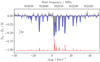 |
Fig. 1 Spectrum of the |

3 Analysis
The presence of amidogen radical in IRAS 16293-2422 was already established by Hily-Blant et al. (2010) during the early phase of the CHESS key program. We used the results obtained in that study for the parent species NH2 to test the validity of our data processing and the subsequent spectral analysis. Figure 1 shows the strongest  component of the fundamental NKa, Kc = 11,1 − 00,0 transition ofo-NH2 around 952 GHz. Here, most of the hyperfine structure (HFS) components are resolved and the intensity of the absorption lines is well above the 3σ noise level threshold.
The resulting model of the full HFS (plotted with the solid blue line in Fig. 1) was computed using a custom Python3 code, which exploits a similar approach to that of the HFS method implemented in CLASS. In contrast to the CLASS method, our code uses the column density (N) and the excitation temperature (Tex) as fit parameters, and the total opacityof the transition (τ) is regarded as a derived quantity. To this aim, the routine makes use of the physical line parameters and implements the computation of the rotational partition function for any given Tex The set of the fit parameters also includes the line systemic velocity (v0) in the local standard of rest and the full-width half maximum (FWHM) of the lines (Δv). Briefly, the total line opacity for a given input is first calculated through:
![\begin{equation*}\tau\,{=}\,\sqrt{\frac{\ln 2}{16\pi^3}}\: \frac{c^3 A_{ul} g_u N}{\nu^3 Q_{\textrm{rot}}(T_{\textrm{ex}}) \Delta\varv} \exp\left(\frac{-E_{\textrm{low}}}{k_{\textrm{B}} T_{\text{ex}}}\right) \left[1 - \exp\left(\frac{-h\nu_0}{k_{\textrm{B}} T_{\text{ex}}} \right)\right] \,, \end{equation*}](/articles/aa/full_html/2020/09/aa38490-20/aa38490-20-eq2.png) (1)
(1)
where ν0 is the rest frequency of the (unsplit)rotational transition, c is the speed of light, Qrot(Tex) is the rotational partition function at Tex, gu is the degeneracy of the upper level, Aul is the Einstein coefficient for spontaneous emission, Elow is the energy of the lower state, h is the Planck constant, and kB is the Boltzmann constant. Then, assuming the local thermodynamic equilibrium (LTE) approximation and Gaussian profiles, the opacity of the ith HFS components is computed as τi = τ Ri, where Ri is the corresponding normalized relative intensity. The ith component opacity at each velocity channel is then given by:
![\begin{equation*}\tau_i(\varv)\,{=}\,\tau_i\,\exp\left[-4\ln 2 \left(\frac{\varv - \varv_{0,i}}{\Delta\varv}\right)^2\right] \,, \end{equation*}](/articles/aa/full_html/2020/09/aa38490-20/aa38490-20-eq3.png) (2)
(2)
where v0,i is the corresponding velocity position expressed as an offset with respect to the systemic velocity v0 Finally, the continuum-subtracted antenna temperature at a given velocity channel v is modeled as
![\begin{equation*}T_{\text{ant}}(\varv)\,{=}\,\left[ J_{\nu} \left(T_{\text{ex}}\right) - J_{\nu} \left(T_{\text{CMB}}\right) - T_{\textrm{C}} \right] \left(1 - \textrm{e}^{-\sum_i\tau_i(\varv)}\right) \,, \end{equation*}](/articles/aa/full_html/2020/09/aa38490-20/aa38490-20-eq4.png) (3)
(3)
where Jν(T) is the Rayleigh–Jeans radiation temperature, TC is the temperatureof the continuum, and TCMB is the cosmic background temperature. These data were compared to the continuum-subtracted observed antenna temperatures, TA − TC, in a non-linear least-squares fashion to determine the best fit values of N, Tex, Δv, and v0 Whenever possible, all four parameters were adjusted during the analysis. This sometimes produced a strong correlation between them, especially when fitting weak features (e.g., those of ND2), for which the relative intensities of the observed HFS components are poorly constrained because of the low signal-to-noise ratio (S/N). In these cases, suitable assumptionsfor Tex and Δv had to be used and the corresponding parameters were kept fixed in the least-squares fit. The single-sideband continuum temperature TC, inserted in the radiative transfer equality of Eq. (3), was estimated using the linear formula given by Hily-Blant et al. (2010), TC ∕[K] = 1.10 ν − 0.42, with ν expressed in THz.
The spectroscopic data for NH2, NHD, and ND2 were taken from the most recent laboratory studies (Martin-Drumel et al. 2014; Bizzocchi et al. 2020; Melosso et al. 2017), and the Qrot values used in Eq. (1) were computed at any given temperature by cubic interpolation on a grid of finely spaced entries spanning the 2.7–19 K interval. These were obtained by direct summation on all rotational levels through the SPCAT spectral tool (Pickett 1991), with the ortho and para species of the symmetric isotopologues NH2 and ND2 treated separately. A brief explanation of the energy level structures of NHD and ND2 is given in Appendix A, while the complete list of HFS components used for the analysis of each transition is reported in Appendix C. The partition function values of both species computed at temperatures between 2.725 and 300 K are given in Appendix B.
Summary of the transitions observed for NH2, NHD, and ND2 toward IRAS16293-2422
4 Results
The line parameters obtained from the analysis of the observed transitions of NH2, NHD, and ND2 are collected in Table 1. In the first two rows, the results obtained for the fine-structure line of o-NH2 previously detected by Hily-Blant et al. (2010) are reported. Our fitted N and Tex values compare very well with those obtained from the CLASS HFS method employed in that study. Our weighted average of the column density is (5.4 ± 0.4) × 1013 cm−2, which is consistent with the value of (4.4 ± 0.7) × 1013 cm−2 obtained previously. The excitation temperatures determined for the two components are 1σ coincident (8.44 ± 0.12 K on average) and are also close to the ones obtained by Hily-Blant et al. (2010) (8.5 K for the  and 9.5 K for
  ).
).
In the same spectral survey, we detect, for the first time, two groups of hyperfine transitions belonging to the singly deuterated form of the amidogen radical, NHD. Figure 2 shows the two fine-structure components of the fundamental NKa,Kc = 11,1 ← 00,0 transition ofNHD, both observed in absorption around 770 and 776 GHz in the 2b HIFI band.
Since the  fine-structure line is detected at the ca. 10σ level, we could adjust all four parameters in the model. The
  component is about twice as weak and its detection is only at the ca. 5σ level. In this case, the noise prevented usfrom adjusting Tex and Δv, which were then fixed at the values obtained for the strongest component of the fine-structure doublet. For NHD, we find an excitation temperature of 7.4 ± 0.1 K, slightly lower than that of NH2. This small difference was likely produced by the bigger Herschel beam size in the 2b band (~ 27′′) compared to that in the 4a band (~ 22′′). Indeed, a larger region is sampled for the NHD lines, and the contribution of the inner warmer gas is expected to be slightly smaller. The average value of the column density is N = (4.7 ± 0.7) × 1013 cm−2
Compared to the parent isotopologue, the doubly deuterated form of amidogen has a denser spectrum in the submillimeter region, thus both the NKa, Kc = 11,1 ← 00,0 and NKa, Kc = 21,2 ← 10,1 rotational lines fall within the coverage of the CHESS spectral survey. A clear detection was obtained in the 2b band for both the  and
and  fine-structure components of the NKa, Kc = 21,2 ← 10,1 transitions of the para species. They are shown in Fig. 3. The NKa, Kc = 11,1 ← 00,0,
  of the ortho species, illustrated in Fig. 4, is located at 527 GHz.
In this spectral region, covered by the HIFI 1a band, the continuum emission of the source is only 200 mK; hence, the resulting absorption feature is rather faint and the detection is only marginal, reaching at most 5σ The other fine-structure component (intrinsically less intense) is just below the noise level and is not detected. Given the weakness of all three components observed for ND2, their analysis had to be carried out by adopting suitable assumptions for Tex and Δv, as these parameters could not be set as free in the least-squares fits. Given the similarity of the beam size (~ 27′′) for the p-ND2 NKa, Kc = 21,2 ← 10,1 lines, we assumed the same excitation temperature as determined for NHD. A smaller value was expected to hold for the o-ND2 NKa, Kc = 11,1 ← 00,0 line, as the Herschel’s half-power beam width (HPBW) at this frequency is as broad as 40′′, thus sampling a comparatively large volume of cold gas. For this transition we fixed Tex = 4.5 K, a value determined for ND in the same source (Bacmann et al. 2010), through the analysis of its N = 1−0 fine-structure doublet centered at 534 GHz. In fact, this value allows for a satisfactory fit of the absorption o-ND2 feature, whereas for higher excitation temperatures (e.g., already at 5.5 K) the LTE model predicts theline to be observable in emission. Constraints for the FWHM line width Δv were derived from the values determined for NH2 after deconvolution from the WBS resolution (1.1 MHz). The column densities derived for p-ND2 using two components are consistent within 2σ, and the weighted average value is N = (0.241 ± 0.014) × 1013 cm−2 The observed ortho-to-para ratio is 2.7 ± 0.4 By considering (i) as the energy difference of 10.77 cm−1 (E∕k ≈ 15.5 K) between the lowest para and ortho rotational levels, and (ii) as the spin statistical weights, this ratio corresponds to an equilibrium temperature of 9 ± 1 K Due to the different beam sizes used to observe the NKa, Kc = 11,1 ← 00,0, and 21,2 ← 10,1 transitions, the p-ND2 is preferentially sampled in the inner warmer region; therefore, this value is likely to be slightly overestimated.
For the same reason, the evaluation of the abundance ratios between amidogen isotopologues requires some careful considerations. From the averaged N values, we obtained [NHD]/[NH2] = 0.87 ± 0.14, hinting at a very high deuteration level for amidogen lying in the 70–100% range. We consider this result to be robust. The HPBW of the observations differs by only 25%, thus the source area sampled by the antenna is similar for both the NHD and NH2 lines. Furthermore, the energy difference between ortho and para species of NH2 is 21.11 cm−1 (E∕kB ≈ 30.4 K), and the contribution of the unobserved p-NH2 is expected to be less than 5% at 10 K Finally, since the used transitions have their lower level located at “zero” energy, the product of two exponential terms in Eq. (1) tends to 1 for small hν0 ∕kBTex, and the relation between N and τ depends only moderately on the temperature. Hence, the retrieved column density values are not much affected by the inaccuracies in the corresponding Tex determination.
The derivation of sound values of the isotopic ratios involving ND2 is less straightforward, as various approaches can be adopted to estimate the overall ND2 column density from the available observational results. By assuming that the two spin species are in thermal equilibrium, total N values of 0.70 × 10¹³ and 0.98 × 1013 cm−2 can be obtained from the o-ND2 and p-ND2 results, respectively. A direct sum of the ortho and para column densities with no assumptions gives instead 0.90 × 1013 cm−2 Based on the resulting 30% discrepancies, we conservatively quote N = (0.9 ± 0.3) × 1013 cm−2 as the total column density of ND2 This yields [ND2]/[NHD] = 0.19 ± 0.07 and [ND2]/[NH2] = 0.17 ± 0.06, that is, deuteration levels in the 10–30% range. The amidogen D/H ratio measured in the low-mass protostar IRAS16293 is very high and is comparable to the one derived for the related species imidogen ([ND]/[NH] = 30−70%, Bacmann et al. 2010), while ammonia shows a lower level ([NH2D]/[NH3] ~ 10%, van Dishoeck et al. 1995). The ND2 species is very abundant, yielding a remarkably high deuteration ratio, even higher than the one found for methanol ([CHD2OH]/[CH3OH] = 6%, Parise et al. 2004), a species for which the triply deuterated species was also detected in this source.
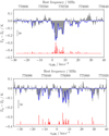 |
Fig. 2 Spectra of the fine components of the NKa,Kc = 11,1 ← 00,0 NHD transition observed toward IRAS 16293-2422 Upper panel: |


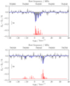 |
Fig. 3 Spectra of the fine-structure components of the NKa,Kc = 21,2 ← 10,1 p-ND2 transition observed toward IRAS 16293-2422 Upper panel: |


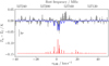 |
Fig. 4 Spectrum of the |

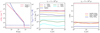 |
Fig. 5 Left panel: density (red) and temperature (blue) structure in the IRAS16293 source model in stages 1 and 2 (see Sect. 5 for details). Middle panel: modeled beam-convolved molecular column densities (solid lines, labeled in the plot) as functions of time in stage 2. Dashed lines represent the observed values, omitting error bars for clarity. Right panel: modeled D/H ratios (solid lines, labeled in the plot) as functions of time in stage 2. Here, the NH2 and ND2 abundances have been summed over the ortho and para forms. Dashed lines represent the observed values, for which the error bars have again been omitted. |
5 Chemical simulation
A steady-state model of cold and CO-depleted clouds was published by Roueff et al. (2005), but their predictions on deuterium enhancement (i.e., 10% for NHD and less than 1% for ND2) are significantly underestimated with respect to our findings, which are 87 and 18% for NHD and ND2, respectively.
In an effort to reproduce the observed tendencies of the D/H and spin-state abundance ratios, we carried out new chemical simulations of (deuterated) amidogen using a model of IRAS 16293-2422 We followed the approach described in Brünken et al. (2014) and Harju et al. (2017), where more details can be found; we provide only a brief description of the simulations here. For the source model, we adopted the one used in the above references, where the physical model from Crimier et al. (2010), which represents the protostellar core, was extended with a layer of gas representing the molecular cloud that the protostellar system lies within (with n(H2) = 104 cm−3 and Tdust = Tgas = 10 K). The source model is illustrated in Fig. 5. We considered a two-stage model, in which the chemical evolution was first calculated over time t1 in physical conditions corresponding to the core extension (stage 1); then the protostellar core model, including the low-density extension, was run over time t2 (stage 2) using the initial chemical abundances obtained from stage 1. We explored a range of t1 and t2 values to search for the best fit to the observed column densities.
The simulation results depend on how the chemical reactions related to (deuterated) amidogen formation are assumed to proceed. Here we used our gas-grain chemical code (Sipilä et al. 2019a) and ran a parameter-space exploration, testing the effects of multi-layer (three-phase) ice chemistry (Sipilä et al. 2016) and a direct proton-deuteron hop (Sipilä et al. 2019b), as opposed to full scrambling in proton-donation reactions (Sipilä et al. 2015), on the various column densities. As an example of the results, Fig. 5 shows a comparison of the beam-convolved modeled and observed column densities with column density ratios using the multi-layer ice model and full scrambling for proton-donation reactions. The chemical model reproduces the column density of o-NH2 and the ND2/NHD ratio very well, but fails to reproducethe NHD/NH2 ratio or the NHD and (ortho and para) ND2 columndensities. Other parameter combinations instead reproduce the NHD and (ortho and para) ND2 column densities very well, but strongly overpredict the o-NH2 column density. None of the parameter combinations we explored led to the observed level for the NHD/NH2 ratio. The chemical model predicts that most of the NHD column originates near the edge of the protostellar core, where the temperature in the source model (~14 K at the very edge, rising inward; cf. Fig. 5) inhibits NHD production with respect to NH2. Indeed, an NHD/NH2 ratio of unity or above can be produced by the chemical model if the gas is sufficiently dense (n(H2) ≳ 105 cm−3) and cold (T ~ 10 K), suggesting that our two-phase approach to the core modeling is inadequate for the modeling of amidogen chemistry, and that a substantial amount of time (on the order of 106 yr) is required in the pre-stellar phase for the NHD/NH2 ratio to increase to the observed level. We stress that in the present work we did not carry out radiative transfer simulations of the amidogen absorption lines, and therefore the comparison of the modeled column densities against the observed ones does not take into account any excitation effects. We will present an in-depth comparison of the model versus the observations in an upcoming work, where we will also carry out line simulations.
6 Discussion and conclusions
This work presents the very first detection of both deuterated forms of amidogen radical in the ISM. Column densities and deuterium fractionation values were derived from the observations, allowing for a direct comparison with the predictions obtained from chemical networks. We ran a parameter-space exploration using our gas-grain chemical code, implementing a two-stage approach to the dynamical evolution of the source. The observed abundances of all NH2, NHD, and ND2 isotopic variants could not be simultaneously reproduced with a single set of modeling parameters, indicating that the two-stage approach to the core modeling is inadequate for simulating amidogen isotopic chemistry. More insights on this topic would come from additional observations of deuterated amidogen isotopologues. The observations are, however, partially hampered by the atmospheric opacity. In fact, the most intense transition of NHD, located at 770 GHz, is not accessible with the ground-based facilities because of strong water absorption lines nearby. Hence, NHD observations can rely mainly on the a-type NKa, Kc = 10, 1 ← 00, 0 transition around 413 GHz. Luckily, spectral coverage at this frequency is supported by the ALMA 8 Band and the new nFLASH receiver of APEX. As for ND2, the transitions detected in this work fall in spectral windows accessible either with the incoming band 1 of the 4GREAT receiver on board SOFIA (490–635 GHz) or the ALMA 10 Band (787– 950 GHz).
The conclusions of the present work can be summarized as follows:
- 1.
Thanks to the recently obtained laboratory data, two deuterated forms of amidogen radical, namely NHD and ND2, were identified for the first time in the ISM. The analysis of hyperfine resolved transitions, observed in absorption against the continuum of the Class 0 protostar IRAS 16293-2422, allowed for the accurate determination of column densitiesand excitation temperatures.
- 2.
The deuterium fractionation of amidogen results to be 70–100% for NHD and 10–30% for ND2. Our derived values differ significantly, being larger by about one order of magnitude, from those predicted by earlier astrochemical models.
- 3.
The low temperature and the high degree of deuteration observed suggest that amidogen, similar to other nitrogen-containing species, is less depleted and subsists longer in the gas-phase, thus leading to high abundances of NHD and ND2.
- 4.
The amidogen D/H and spin-state abundance ratios in IRAS 16293-2422 cannot be reproduced with our gas-grain chemicalmodel unless the pre-stellar stage has a long duration, on the order of one million years.
- 5.
The best candidate to perform future observations of NHD and ND2, not only in IRAS 16293-2422 but also in other sources where deuterated ammonia has been detected, is ALMA. More observations would enable us to take a step toward a thorough understanding of ammonia formation and deuteration in the ISM.
Acknowledgements
This study was supported by Bologna University (RFO funds) and by MIUR (Project PRIN 2015: STARS in the CAOS, Grant Number 2015F59J3R). The work at SOLEIL was supported by the Programme National “Physique et Chimie du Milieu Interstellaire” (PCMI) of CNRS/INSU with INC/INP co-funded by CEA and CNES.
Appendix A: Energy level scheme
A.1 Singly deuterated amidogen radical
The manifold of rotational energy levels is very complex in NHD and its spectrum is characterized by many interactions. First, NHD is a light asymmetric rotor far from the prolate limit (κ = −0.66), whose electric dipole moment lies in the ab principal symmetry plane, with components μa = 0.67 D and μb = 1.69 D (Brown et al. 1979). Because of the large values of the rotational constants, the room temperature spectrum is quite sparse and peaks in the far-infrared (FIR) region.
Furthermore, NHD is an open-shell molecule with an  ground electronic state. Due to the presence of an unpaired electron, the electronic spin (S = 1∕2) couples with the rotational angular momentum N, thus splitting each rotational level
  into two fine-structure sub-levels. The fine-structure levels have either J = N +1∕2 or J = N −1∕2 quantum numbers, with the exception of the N = 0 level, for which only the J = 1∕2 level exists. The total angular momentum J further couples witheach nuclear spin (IN and ID = 1, IH = 1∕2), giving rise to the so-called hyperfine structure (HFS). The adopted angular momentum coupling scheme takes into account the magnitude of the interaction (from strongest to weakest):

A more detailed account of the NHD spectroscopy can be found in Bizzocchi et al. (2020).
A.2 Doubly deuterated amidogen radical
The higher symmetry of ND2 with respect to NHD requires additional considerations in the description of the energy level manifold. The species ND2 belongs to the C2v symmetry point group, and a π-rotation along the b axis exchanges the two identical deuterium nuclei. Since deuterium is a boson, the total wave-function of ND2 must be symmetric upon the permutation of the two particles. Given that the electronic ground state is antisymmetric ( ) and the vibrational ground state is symmetric, deuterium nuclear spin functions (
 ) can only combine with rotational levels of opposite symmetry. That is, symmetric rotational levels (Ka + Kc = even) combine with antisymmetric deuterium spin functions with ID, tot = 1 (ortho states), while antisymmetric rotational levels (Ka + Kc = odd) combine with the spin functions ID, tot = 0, 2 (para states). Only transitions within the states are allowed by the permanent electric dipole moment of ND2 (μb = 1.82(5) D Brown et al. 1979). At low temperatures, given the energy difference of 15.5 K between the ortho and para states, o-ND2 and p-ND2 should be considered as different species.
The network of fine and hyperfine interactions in ND2 is analogous to that described earlier for NHD, while the coupling scheme of angular momentum changes as follows:

A detailed account of the spectroscopic features of ND2 can be found in Melosso et al. (2017).
Appendix B: Partition function values
The spectroscopic parameters from Bizzocchi et al. (2020) and Melosso et al. (2017) were input into the SPCAT subroutine (Pickett 1991) to evaluate the rotational partition function of NHD and ND2, respectively. All energy levels up to J = 20 and Ka = 15 were considered. The temperature-dependence of Qrot was computed analytically for both species at temperatures between 2.725 and 300 K. These values are given in Table B.1.
Rotational partition function values of NHD and ND2 computed at different temperatures.
Appendix C: List of the used HFS components
Tables C.1–C.5 list the rest frequencies of the observed hyperfine components of NHD and ND2. The LTE intensities (computed at 300 K and labeled LGINT in the tables) and the HFS quantum numbers are also given. Spectral predictions are based on the spectroscopic studies reported in Melosso et al. (2017) and in Bizzocchi et al. (2020).
HFS components used to reproduce the  transition of NHD.
HFS components used to reproduce the  transition of NHD.
HFS components used to reproduce the  transition of ND2.
HFS components used to reproduce the  transition of ND2.
HFS components used to reproduce the  transition of ND2.
References
- Bacmann, A., Caux, E., Hily-Blant, P., et al. 2010, A&A, 521, L42 [NASA ADS] [CrossRef] [EDP Sciences] [Google Scholar]
- Bacmann, A., Daniel, F., Caselli, P., et al. 2016, A&A, 587, A26 [NASA ADS] [CrossRef] [EDP Sciences] [Google Scholar]
- Bizzocchi, L., Melosso, M., Giuliano, B. M., et al. 2020, ApJS, 247, 59 [CrossRef] [Google Scholar]
- Brown, J., Chalkley, S., & Wayne, F. 1979, Mol. Phys., 38, 1521 [NASA ADS] [CrossRef] [Google Scholar]
- Brünken, S., Sipilä, O., Chambers, E. T., et al. 2014, Nature, 516, 219 [NASA ADS] [CrossRef] [PubMed] [Google Scholar]
- Butner, H., Charnley, S., Ceccarelli, C., et al. 2007, ApJ, 659, L137 [NASA ADS] [CrossRef] [Google Scholar]
- Caselli, P., & Ceccarelli, C. 2012, A&ARv, 20, 56 [Google Scholar]
- Ceccarelli, C., Castets, A., Loinard, L., Caux, E., & Tielens, A. 1998, A&A, 338, L43 [Google Scholar]
- Ceccarelli, C., Caselli, P., Herbst, E., Tielens, A. G. G. M., & Caux, E. 2007, in Protostars and Planets V, eds. B. Reipurth, D. Jewitt, & K. Keil (Tucson, AZ: University of Arizona Press), 47 [Google Scholar]
- Ceccarelli, C., Bacmann, A., Boogert, A., et al. 2010, A&A, 521, L22 [NASA ADS] [CrossRef] [EDP Sciences] [Google Scholar]
- Ceccarelli, C., Caselli, P., Bockelée-Morvan, D., et al. 2014, Protostars and Planets VI (Tucson, AZ: University of Arizona Press), 859 [Google Scholar]
- Comito, C., & Schilke, P. 2002, A&A, 395, 357 [NASA ADS] [CrossRef] [EDP Sciences] [Google Scholar]
- Crimier, N., Ceccarelli, C., Maret, S., et al. 2010, A&A, 519, A65 [NASA ADS] [CrossRef] [EDP Sciences] [Google Scholar]
- de Graauw, T., Helmich, F. P., Phillips, T. G., et al. 2010, A&A, 518, L6 [NASA ADS] [CrossRef] [EDP Sciences] [Google Scholar]
- Fayolle, E. C., Öberg, K. I., Jørgensen, J. K., et al. 2017, Nat. Astron., 1, 703 [NASA ADS] [CrossRef] [Google Scholar]
- Harju, J., Sipilä, O., Brünken, S., et al. 2017, ApJ, 840, 63 [NASA ADS] [CrossRef] [Google Scholar]
- Hily-Blant, P., Maret, S., Bacmann, A., et al. 2010, A&A, 521, L52 [NASA ADS] [CrossRef] [EDP Sciences] [Google Scholar]
- Jørgensen, J. K., Favre, C., Bisschop, S. E., et al. 2012, ApJ, 757, L4 [NASA ADS] [CrossRef] [Google Scholar]
- Kanada, M., Yamamoto, S., & Saito, S. 1991, J. Chem. Phys., 94, 3423 [CrossRef] [Google Scholar]
- Kobayashi, K., Ozeki, H., Saito, S., Tonooka, M., & Yamamoto, S. 1997, J. Chem. Phys., 107, 9289 [NASA ADS] [CrossRef] [Google Scholar]
- Linsky, J. L. 2003, in Solar System History from Isotopic Signatures of Volatile Elements (Berlin: Springer), 49 [CrossRef] [Google Scholar]
- Loinard, L., Castets, A., Ceccarelli, C., Caux, E., & Tielens, A. 2001, ApJ, 552, L163 [NASA ADS] [CrossRef] [Google Scholar]
- Martin-Drumel, M. A., Pirali, O., & Vervloet, M. 2014, J. Phys. Chem. A, 118, 1331 [CrossRef] [Google Scholar]
- Melosso, M., Degli Esposti, C., & Dore, L. 2017, ApJS, 233, 1 [CrossRef] [Google Scholar]
- Melosso, M., Bizzocchi, L., Tamassia, F., et al. 2019a, Phys. Chem. Chem. Phys., 21, 3564 [CrossRef] [Google Scholar]
- Melosso, M., Conversazioni, B., Degli Esposti, C., et al. 2019b, J. Quant. Spectr. Rad. Transf., 222, 186 [CrossRef] [Google Scholar]
- Melosso, M., Dore, L., Gauss, J., & Puzzarini, C. 2020, J. Mol. Spectr., 370, 111291 [CrossRef] [Google Scholar]
- Ott, S. 2010, ASP Conf. Ser., 434, 139 [Google Scholar]
- Parise, B., Castets, A., Herbst, E., et al. 2004, A&A, 416, 159 [NASA ADS] [CrossRef] [EDP Sciences] [Google Scholar]
- Pickett, H. M. 1991, J. Mol. Spectr., 148, 371 [NASA ADS] [CrossRef] [Google Scholar]
- Roelfsema, P. R., Helmich, F. P., Teyssier, D., et al. 2012, A&A, 537, A17 [NASA ADS] [CrossRef] [EDP Sciences] [Google Scholar]
- Roueff, E., Lis, D. C., Van der Tak, F., Gerin, M., & Goldsmith, P. 2005, A&A, 438, 585 [NASA ADS] [CrossRef] [EDP Sciences] [Google Scholar]
- Sipilä, O., Harju, J., Caselli, P., & Schlemmer, S. 2015, A&A, 581, A122 [NASA ADS] [CrossRef] [EDP Sciences] [Google Scholar]
- Sipilä, O., Caselli, P., & Taquet, V. 2016, A&A, 591, A9 [NASA ADS] [CrossRef] [EDP Sciences] [Google Scholar]
- Sipilä, O., Caselli, P., Redaelli, E., Juvela, M., & Bizzocchi, L. 2019a, MNRAS, 487, 1269 [Google Scholar]
- Sipilä, O., Caselli, P., & Harju, J. 2019b, A&A, 631, A63 [CrossRef] [EDP Sciences] [Google Scholar]
- van der Tak, F. F. S., Schilke, P., Müller, H. S. P., et al. 2002, A&A, 388, L53 [NASA ADS] [CrossRef] [EDP Sciences] [Google Scholar]
- van Dishoeck, E. F., Blake, G. A., Jansen, D. J., et al. 1995, ApJ, 447, 760 [NASA ADS] [CrossRef] [Google Scholar]
- Vastel, C., Phillips, T., Ceccarelli, C., & Pearson, J. 2003, ApJ, 593, L97 [NASA ADS] [CrossRef] [Google Scholar]
ESA Herschel Science Archive http://archives.esac.esa.int/hsa/whsa.
See GILDAS home page at the URL: http://www.iram.fr/IRAMFR/GILDAS.
All Tables
Rotational partition function values of NHD and ND2 computed at different temperatures.
All Figures
|
Fig. 1 Spectrum of the |
| In the text | |
|
Fig. 2 Spectra of the fine components of the NKa,Kc = 11,1 ← 00,0 NHD transition observed toward IRAS 16293-2422 Upper panel: |
| In the text | |
|
Fig. 3 Spectra of the fine-structure components of the NKa,Kc = 21,2 ← 10,1 p-ND2 transition observed toward IRAS 16293-2422 Upper panel: |
| In the text | |
|
Fig. 4 Spectrum of the |
| In the text | |
|
Fig. 5 Left panel: density (red) and temperature (blue) structure in the IRAS16293 source model in stages 1 and 2 (see Sect. 5 for details). Middle panel: modeled beam-convolved molecular column densities (solid lines, labeled in the plot) as functions of time in stage 2. Dashed lines represent the observed values, omitting error bars for clarity. Right panel: modeled D/H ratios (solid lines, labeled in the plot) as functions of time in stage 2. Here, the NH2 and ND2 abundances have been summed over the ortho and para forms. Dashed lines represent the observed values, for which the error bars have again been omitted. |
| In the text | |
Current usage metrics show cumulative count of Article Views (full-text article views including HTML views, PDF and ePub downloads, according to the available data) and Abstracts Views on Vision4Press platform.
Data correspond to usage on the plateform after 2015. The current usage metrics is available 48-96 hours after online publication and is updated daily on week days.
Initial download of the metrics may take a while.