| Issue |
A&A
Volume 641, September 2020
|
|
|---|---|---|
| Article Number | A91 | |
| Number of page(s) | 8 | |
| Section | Stellar structure and evolution | |
| DOI | https://doi.org/10.1051/0004-6361/202038110 | |
| Published online | 15 September 2020 | |
Long photometric cycle and disk evolution in the β Lyrae-type binary OGLE-BLG-ECL-157529
1
Universidad de Concepción, Departamento de Astronomía, Casilla 160-C, Concepción, Chile
e-mail: This email address is being protected from spambots. You need JavaScript enabled to view it.
2
Astronomical Observatory, Volgina 7, 11060 Belgrade 38, Serbia
3
Issac Newton institute of Chile, Yugoslavia Branch, 11060 Belgrade, Serbia
4
Astronomical Observatory, University of Warsaw, Al. Ujazdowskie 4, 00-478 Warszawa, Poland
Received:
7
April
2020
Accepted:
25
June
2020
Abstract
Context. The subtype of hot algol semidetached binaries dubbed double periodic variables (DPVs) are characterized by a photometric cycle longer than the orbital one, whose nature has been related to a magnetic dynamo in the donor component controlling the mass transfer rate.
Aims. We aim to understand the morphologic changes observed in the light curve of OGLE-BLG-ECL-157529 that are linked to the long cycle. In particular, we want to explain the changes in the relative depth of primary and secondary eclipses.
Methods. We analyzed I and V-band OGLE photometric times series spanning 18.5 years and modeled the orbital light curve.
Results. We find that OGLE-BLG-ECL-157529 is a new eclipsing Galactic DPV of orbital period 24d.8, and that its long cycle length decreases in amplitude and length during the time baseline. We show that the changes in the orbital light curve can be reproduced considering an accretion disk of variable thickness and radius that surrounds the hottest stellar component. Our models indicate changes in the temperatures of the hot spot and the bright spot during the long cycle, and also in the position of the bright spot. This, along with the changes in disk radius, might indicate a variable mass transfer in this system.
Key words: binaries: close / binaries: eclipsing / stars: variables: general / accretion, accretion disks
© ESO 2020
1. Introduction
Double periodic variables (DPVs) are a subset of Algol-type binary systems. They consist of a red giant that has filled its Roche lobe and transfers material through an optically thick accretion disk onto a B-type dwarf. Their main characteristic is that they have two photometric cycles: a short period Po, whose light curve shape is typical of the orbital modulation in eclipsing or ellipsoidal binaries, and a long cycle period Pl, whose origin is still unknown. Both periodicities are related through the relationship Pl = 33 × Po, but the period ratio for a particular case can differ considerably from the average (Mennickent et al. 2003a, 2016; Poleski et al. 2010; Pawlak et al. 2013; Mennickent 2017). In some systems, a decrease in the long period has been reported, as in the case of OGLE-LMC-DPV-065 (Poleski et al. 2010; Mennickent et al. 2019) and OGLE-LMC-DPV-056 (Mennickent et al. 2003b).
A magnetic origin has been proposed as the cause of the long cycle (Schleicher & Mennickent 2017). The rapid rotation of an orbitally synchronized donor star, added to the convective motions, would cause it to have a magnetic dynamo, which would change the equatorial stellar radius as indicated by the Applegate mechanism (Applegate & Patterson 1987; Applegate 1992); this should modulate the mass transfer through the inner Lagrangian point. These changes could be observed as cyclic luminosity variations evidenced in the long cycle. This model, proposed by Schleicher & Mennickent (2017), predicts the correlation between the orbital and long periods and also the value of the long cycle length for particular systems with relatively good accuracy; for the seven studied binaries with orbital periods between 5 and 13 days, the maximum deviation between the predicted and observed ratio is 30%, with the average deviation being on the order of 12%. Actually, it has been shown that rapid rotation favors the operation of the Applegate mechanism (Navarrete et al. 2018).
Other mechanisms have been identified as drivers for mass transfer changes in close binaries. These include direct modulation of mass transfer through the magnetic field of the donor star (Bolton 1989; Meintjes 2004) and the effect of star spots or prominences (Livio & Pringle 1994; Steeghs et al. 1996; Meintjes 2004).
Recently, Mg II, Fe I, Fe II, C I, and Ti II emission lines, which are signatures of chromospherically active stars, were detected in V 393 Scorpii, supporting the existence of magnetically active donors in DPVs (Mennickent et al. 2018). In addition, magnetic fields have been inferred in β Lyrae from the analysis of polarized light that could produce magnetically driven streams onto the accretion disk (Skulskij 1982, 2018).
Significant changes have been detected in the morphology of the light curve of OGLE-LMC-DPV-097 that are directly related to the long cycle (Garcés et al. 2018). These authors show that this kind of variability could be due to physical changes of the accretion disk, which would change its diameter and thickness cyclically according to the phase of the long cycle. If the long cycle reflects changes in the mass transfer rate, we might expect changes in disk properties too, since the disk interacts with the gas stream.
In this study we show the photometric analysis of a Galactic DPV binary system that presents a variable long cycle, namely OGLE-BLG-ECL-157529 (α2000 = 17:53:08.33, δ2000 = −32:46:27.0, I = 13.035 mag, V = 14.829 mag, Soszyński et al. 2016). It is the first DPV reported in the direction of the Galactic bulge. The Gaia data release 2 identification is 4043437999622564608 and its parallax is 0.331 ± 0.044 mas, implying a distance of 3024 ± 406 pc (Gaia Collaboration 2016, 2018). This distance fits well with that provided by Bailer-Jones et al. (2018): 2815 pc with a lower limit at 2487 pc and an upper limit at 3240 pc. The above indicates that the system is not a member of the Galactic bulge, but a foreground star.
We used good time coverage in the OGLE data to study changes in the morphology of the light curve. As in OGLE-LMC-DPV-097, we found the light curve was related to the long cycle. Our motivation is to investigate the physical phenomena that give rise to the peculiar changes observed in the binary system’s orbital light curve, in order to understand the cause of these changes. This object, together with other DPVs that show linked orbital and long cycle variability, could be fundamental in a study aimed at understanding the DPV phenomenon and testing the hypothesis of the magnetic dynamo. A preliminary report of this investigation was presented by Garcés et al. (2019).
2. Photometric data
This object is included in the catalog of eclipsing binaries in the Galactic bulge presented by Soszyński et al. (2016). The photometric time series analyzed in this study consists of 2606 I-band data points taken from the following databases (Fig. 1): OGLE-II (Szymański 2005)1 and OGLE-III/IV2. The OGLE-IV project is described by Udalski et al. (2015). In addition, the OGLE-IV database provides 118 additional V-band measurements. The whole dataset, summarized in Table 1, spans a time interval of 6781 d, or 18.5 yr.
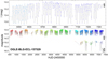 |
Fig. 1. OGLE I and V-band light curves of OGLE-BLG-ECL-157529. Colors indicate different data ranges. |
Summary of photometric observations.
3. Results
In this section we present the results of our analysis of the light curve and also some insights on the system reddening, distance and cooler star.
3.1. Light curve analysis
The light curve shows alternate and periodic minima that are typical of an eclipsing binary system, but also a long cycle on a timescale of several hundreds of days (Fig. 1). The system is fainter in the V-band than in the I-band and the eclipses are deeper in V.
We used the generalized Lomb-Scargle (GLS) periodogram to obtain the orbital frequency in our data. This algorithm was introduced by Zechmeister & Kürster (2009) and uses the principle of the Lomb (1976) and Scargle (1982) periodograms with some modifications, such as the addition of a displacement in the adjustment of the fit function and the consideration of measurement errors. Compared with the classical periodogram, it gives us more accurate frequencies and a better determination of the amplitudes. We obtained 
With the above period we phased the I-band light curve. This allowed us to select the deeper data points in the primary eclipse, corresponding in this system to the usually deeper eclipse, for every data segment that is colored in Fig. 1. These data points were analyzed with the cycle-number technique for linear ephemerides (Sterken 2005) and the following improved ephemeris for the primary eclipse was derived (Fig. 2):
 (1)
(1)
where N is the cycle number. This period was used to phase the light curve shown in Fig. 3. From this figure we infer the following: (1) at some epochs the secondary eclipse becomes deeper than the primary eclipse, (2) the secondary eclipse has larger variability (scatter) than the primary eclipse, (3) the regularity of time strings reflected in the colored data suggests that the non-orbital variability occurs mostly on timescales of hundred of days, (4) while the secondary eclipse changes its depth as well as its width, the primary one primarily changes in depth, and with less amplitude than the secondary eclipse, (5) the long cycle, revealed by the scattered data, becomes more evident outside the primary eclipse, suggesting that the light source becomes at least partially eclipsed during primary eclipse, (6) there is a tendency for the primary eclipse to be deeper with time, and (7) the orbital period seems to be very stable during the observing period.
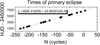 |
Fig. 2. Times of primary eclipse that provide an improved value for the orbital period |
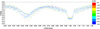 |
Fig. 3. OGLE I-band light curve of OGLE-BLG-ECL-157529 phased with the ephemeris given by Eq. (1). Colors label data shown in Fig. 1. |
We tested the last statement by making an analysis of the times of the primary eclipse using the “period-change equation” (Percy et al. 1980). This method assumes a constant rate of change of the period and compares predicted times with observed times in a similar way to the O–C diagram described by Sterken (2005). As eclipse timings we chose the fainter points in the colored data strings shown in Fig. 3. We find a period rate of change of dPo/dt = (1.41 ± 1.38) × 10−5 d d−1, meaning the period is constant for all practical purposes (Fig. 4). We find that the eclipses depth changes linearly with time and in an opposite way during the 18.5-year interval; the total change of the secondary eclipse depth, about 0.35 mag, is larger than the total change of the primary eclipse depth, about 0.10 mag (Fig. 5).
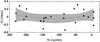 |
Fig. 4. Observed minus calculated times for primary eclipses using the orbital period given by the ephemeris of Eq. (1) and the best fit. The dashed area shows the 95% confidence band. |
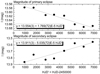 |
Fig. 5. Eclipse magnitudes as a function of time. The lowest point of every colored data segment in the eclipses of Fig. 2 is plotted. |
The long cycle is revealed in the weighted wavelet Z transform (WWZ) as defined by Foster (1996). The WWZ works in a similar way to the Lomb-Scargle periodogram providing information about the periods of the signal and the time associated to those periods. It is very suitable for the analysis of non-stationary signals and has advantages for the analysis of time-frequency local characteristics. The WWZ shows the long period decreasing from around 900 days to around 800 days through the time baseline (Fig. 6).
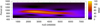 |
Fig. 6. Weighted wavelet Z transform 2D power spectrum as a function of period and time. |
We fit the data segments with sixth order polynomials in order to represent the long cycle. These fits show that the long cycle decreases its period and amplitude during the time baseline (Fig. 7). The continuous smooth decrease of the brightness of the primary eclipse (lower red and blue points, orbital phases around 0 or 1) along with the much fainter secondary eclipses occurring at some epochs (green very low points, orbital phases around 0.5) are clear from this figure. It is also clear how the secondary eclipse becomes brighter as time goes by.
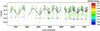 |
Fig. 7. I-band light curve showing the polynomial fits to the long cycle. Colors represent the orbital phases according to the ephemeris given by Eq. (1). We note the evolution of the secondary eclipse (green) and the primary eclipse (red and blue). |
We analyzed the orbital light curves after removing the long cycle. This was done using the residuals of the fits shown in Fig. 7. Examples of “cleaned” orbital light curves are shown in Fig. 8. These show changes in the shape of the orbital light curve that are more evident during the first observing epochs (Fig. 9). In particular, we notice the changes in the shape of the eclipses and the ingress and egress light curve branches. The primary eclipse is not always deeper than the secondary one, this is especially evident in the first observing epochs. We also notice changes in the shape of the light curve during epochs of long cycle maximum and minimum (Fig. 10); during the minima of the long cycle the reversals of the eclipse depths occurs, something already visible in Fig. 7 at the lower parts of the fits.
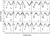 |
Fig. 8. Orbital light curves constructed with residuals of the fits shown in Fig. 7 for data spanning the time interval (HJD-245000) between 6334.9 and 7332.5. Every panel shows 50 consecutive data points. Time goes from left to right from the upper left to the lower right panel. |
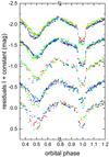 |
Fig. 9. Orbital light curves constructed with the residuals of the fits shown in Fig. 7. Data are grouped for the first fit (lower) until the fifth fit residuals (upper). To illustrate changes in the shape of the light curves, data are marked with a color map following the HJD; red for the first observations and blue for the last observations of every segment. |
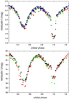 |
Fig. 10. Orbital light curves constructed with the residuals of the fits shown in Fig. 5. Data are grouped for times of maxima (upper) and minima (lower) of the long cycle. The ranges of HJD – 2450000 are: (upper) brown; 3569.8–3629.6, green; 4329.6–4393.5, blue; 5866.5–6023.8, red; 1608.8–1667.8, and black; 6572.6–6816.8, (lower) red; 3049.9–3205.6, black; 3881.7–4028.5, and green; 7064.9–7110.9. |
In order to understand these changes, in the next section we investigate the nature of the star facing the observer during the primary eclipse. This is usually named the donor star in a β-Lyr-type binary, because it transfers mass onto the “gainer” star through a gas stream flowing from its inner Lagrangian point.
3.2. System reddening, distance, and donor star
Since we do not have spectroscopic data for our object, we must use photometry to further understand the system. Using OGLE-IV photometry and the disentangled orbital light curve, we obtain a V − I = 2.42 mag at the primary eclipse. The location of this DPV in the direction of the Galactic bulge causes the light from this object to be strongly reddened by unevenly distributed interstellar matter.
This object is located in the OGLE field BLG535, which is just over three degrees distant from the Galactic plane. In this direction, dust is distributed highly non-uniformly and reddening changes on a small angular scale. Nataf et al. (2013) have estimated reddening using red clump stars located in the Galactic bulge, so reddening measurements from their map are the upper limits toward the analyzed directions, and they should not be used for the objects located definitely closer than the Bulge. In Fig. 11 we show a color-magnitude diagram (CMD) toward the direction of OGLE-BLG-ECL-157529. We use stars located in a radius of about 2.5 arcmin around the position of the analyzed object. In the CMD we mark our target, the red clump (which has a mean position of (V − I), I) = (2.33 mag, 16.11 mag)) and the reddening vector. We use the OGLE Extinction Calculator3 that uses the Nataf extinction maps, and obtain limits for the color excess E(V − I) = 1.266 mag using the nearest method and E(V − I) = 1.248 mag using the natural neighbor method.
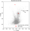 |
Fig. 11. Color-magnitude diagram for stars surrounding OGLE-BLG-ECL-157529. The reddening vector, extinction value, and magnitudes of the red clump are from Nataf et al. (2013). More details can be found in Sect. 3.2. |
As previously mentioned, the Gaia parallax of 0.33065 ± 0.04436 mas implies a distance of d = 3024 ± 406 pc. This means that the object is in the Galactic disk and not in the bulge. Using the Recio-Blanco model for the Galactic disk (Recio-Blanco et al. 2014) along with the Gaia distance we obtain E(V − I) = 0.945 mag implying a dereddened color index of (V − I)0 = 1.475 mag at the primary eclipse. In the previous step we used as input the uncorrected color excess obtained with the natural neighbor method. To complement our research on reddening, we also used the Python package named “mwdust”4 that uses several existing extinction maps in the Milky Way (Bovy et al. 2016). Using this package, we obtain the extinction at a given direction and distance. For a distance of 3.02 kpc we have obtained an extinction in the V- and I-bands of AV = 2.288 mag and AI = 1.256 mag, which gives E(V − I) = 1.033 mag, roughly confirming the earlier calculation.
The corrected color in primary eclipse obtained with the Recio-Blanco model (Recio-Blanco et al. 2014), namely (V − I)0 = 1.47 mag, corresponds to a K2-type star with Tc = 4400 K (Drilling et al. 2000) (Fig. 12). In the following we will assume that this is the effective temperature of the donor star. The relative stability of the primary eclipse might support this conjecture.
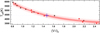 |
Fig. 12. Temperature vs. color for dwarfs (black dots) and giants (red dots) from Drilling et al. (2000) and the best 3th order polynomial fit. Confidence of 95% and prediction bands are shown by dashed and dashed-light areas, respectively. The position of OGLE-BLG-ECL-157529 during the primary eclipse is also shown. |
4. Discussion
In the following we give a qualitative interpretation of the observations, followed by the construction of a model of the system, based on the best fit to the orbital light curve.
4.1. Overall qualitative interpretation
The overall behavior of the light curve, especially the behavior of the secondary eclipse, can be interpreted in terms of the circumstellar material in the system. The changing shape of the secondary eclipse cannot be due to occultation by a star, but by a variable structure such as an accretion disk, which surrounds the more massive star and is formed by mass transfer from the Roche lobe overflow of the less massive star. This configuration is typical of semidetached Algols of the β Lyrae type. What is not typical and is unique for this system is the presence of a large amplitude long photometric cycle and the remarkable changes observed in the relative depths of the primary and secondary eclipses.
From the analysis shown in the previous section we might infer the existence of a large disk during the first observing epochs, but that decreases its size as time goes by. This should explain why the secondary eclipse is deeper at the beginning. This long-term behavior of the disk is reflected in the secondary eclipse magnitude (Fig. 5). When the disk is vertically larger (regarding the orbital plane), it occults a larger fraction of the donor and gainer and the eclipse becomes deeper. However, the deeper secondary eclipses occur only during long-cycle minima, and this should indicate that the disk size is also modulated by the long cycle, but on a shorter timescale as compared with the aforementioned decade-length secular tendency.
We also notice that the disk attains its maximum size when the long cycle has a larger amplitude and its cycle length is longer, which occurs at the beginning of the time series. We suggest that changes in mass transfer control the disk size and eventually the brightness of the extra source responsible for the long cycle. This extra source might be a hot spot wind, as suggested for the DPV system V 393 Scorpii (Mennickent et al. 2012) and also for β Lyrae (Harmanec et al. 1996). Since we do not detect changes in the orbital period, the mass transfer in this system should be rather small.
4.2. Light curve model
In this subsection we model the light curve in order to test the picture of the variable disk given above. We use a theoretical code that solves the inverse problem and that considers a system consisting of a donor star and a gainer star surrounded by an accretion disk, which is both optically and geometrically thick (Djurašević 1992a,b, 1996). The disk temperature is the same as the gainer at its inner edge and decreases with a radial profile described by an exponent aT. The model includes a hot spot and a bright spot in the disk, following evidence found in previous observations of algols (Richards 2004). These active regions influence the shape of the light curve during the ingress and egress of the eclipses. The model has been described in detail in several papers, so we refer the interested reader to Mennickent & Djurašević (2013) and Mennickent et al. (2015, 2019). We assume a donor temperature of Tc = 4400 K, as derived in the previous section. We also assume synchronous rotation for the donor, as expected for a close binary that rapidly synchronizes stellar spins with the orbit due to tidal forces. On the other hand, the gainer might have been spun-up to a high rotation due to the nearly tangential infalling of material (Packet 1981), hence we have assumed critical rotation for this star. We find that our model is practically the same for a synchronous and critical gainer.
We use the q-search method, usually applied to over-contact or semidetached binaries when no spectroscopic data are available (Terrell & Wilson 2005). We find convergent solutions for a range of mass ratios q = Mc/Mh, where the subindexes “c” and “h” refer to the cool and hot stars. A fit with a fourth order polynomial to the corresponding Σ (O − C)2 values, yields an optimal mass ratio of q = 0.22 (Fig. 13). Previous studies show q̅ = 0.23 ± 0.05 (standard deviation) for the few studied DPVs (Mennickent et al. 2016). For the q-search we used data obtained at maximum (Fig. 10 upper), when the disk influence should be lower, as discussed in the previous section.
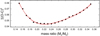 |
Fig. 13. Parameter Σ (O–C)2 for the fits done to the light curve with data obtained at the maximum of the long cycle, as a function of mass ratio. The best 4th order polynomial fit is shown along with the 95% confidence band. |
Next we model the light curve at data ranges representative of the maximum and minimum of the long cycle. We choose those data ranges that best represent the observed differences between maximum and minimum, where the inversion of the eclipses is more evident. The parameters of the fits are shown in Table 2 and a comparison of our theoretical models and observations is given in Fig. 14. While the models reproduce relatively well the general appearance of the light curves, the fit at minimum has more scatter than at maximum. It is possible that at minimum the emissivity sources are more complex and our simple model of the disk plus spots cannot reproduce the overall system emissivity very well.
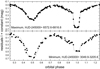 |
Fig. 14. Orbital light curves at long cycle maximum and minimum along with the fits provided by the models described in Table 2. |
4.3. Discussion of the light curve models
Our model suggests a system seen at angle 85° and a stellar separation of 65 R⊙. The stellar temperatures are 4400 K and 14.000 K. The stellar masses are 4.83 and 1.06 ℳ⊙, and the surface gravities are log g = 3.86 and 2.02. The stellar radii are 4.5 and 16.6 R⊙. The gainer has a surface temperature indicating a B 6 spectral type (Harmanec 1988), consistent with the B-type spectral types found in DPV gainers. Although we have justified the use of the fixed parameters Tc and q, the stellar parameters might be refined when spectroscopic data come to be available.
Significant differences are observed in disk properties when passing from the maximum to the minimum of the long cycle: the radius increases from 27 to 33 R⊙, while the temperature at the outer edge remains around 3000–3500 K. The vertical thickness at the outer edges increases from 3 to 11 R⊙, which explains the inversion of the eclipse depths. The average disk radius of 30 R⊙ means Rd/a ≈ 0.47, meaning the outer border of the disk is just below the tidal radius for the given mass ratio (Paczyński 1977; Warner 1995a). This opens the possibility that at minimum the outer disk, especially optically thin regions that are not tested with our light curve model, becomes influenced by tidal forces. The light contribution of the larger disk explains the shallower primary eclipse observed at the first epochs (red points in Fig. 3).
The bright spot is located roughly at the expected region where the stream impacts the disk, 47° apart from the lines joining the stellar centers in the direction of the orbital motion. This position does not change between maximum and minimum. On the contrary, the position of the bright spot changes from 66° to 125° from maximum to minimum, as measured in the opposite direction from the orbital motion. At maximum the hot spot temperature is 48% higher than the surrounding disk, at minimum it is only 13% higher, which in principle is consistent with a large amount of kinetic energy being released in the stream-disk impact region in a smaller disk. At maximum the bright spot temperature is 37% higher than the surrounding disk and 8% at minimum. We notice that changes in the disk parameters, especially the disk radius and the temperatures of the active regions, might indicate variable mass transfer in the system, as required in the dynamo model proposed by Schleicher & Mennickent (2017).
5. Conclusion
We find that the eclipsing binary OGLE-BLG-ECL-157529 is a double periodic variable characterized by an orbital period of 24 80091 ± 0
 00044 and a long cycle length decreasing in length and amplitude during 18.5 years of observations.
The overall light curves can be understood in terms of a variable accretion disk. The disk is larger and thicker at the long cycle minimum and this effect is more pronounced when the long cycle has a larger amplitude and a longer cycle length.
Our models indicate changes in the temperatures of the hot spot and the bright spot during the long cycle, and also in the position of the bright spot. This, along with the changes in disk radius, might indicate variable mass transfer in this system.
OGLE-III/IV data kindly provided by the OGLE team.
Acknowledgments
We thanks the anonymous referee who contributed to improve the first version of this manuscript. REM and JG acknowledge support by VRID-Enlace 216.016.002-1.0, BASAL Centro de Astrofísica y Tecnologías Afines (CATA) PFB–06/2007 and FONDECYT 1190621. DS and REM thank FONDECYT 1201280 and DS thanks FONDECYT 1161247. JG acknowledges ANID project 21202285 and members of stellar variability group (S. V. G. UdeC) for useful discussions about this work. GD acknowledges the financial support of the Ministry of Education, Science and Technological Development of the Republic of Serbia through the contract No 451-03-68/2020/14/20002. The OGLE project has received funding from the Polish National Science Centre grant MAESTRO no. 2014/14/A/ST9/00121. This work has made use of data from the European Space Agency (ESA) mission Gaia (https://www.cosmos.esa.int/gaia), processed by the Gaia Data Processing and Analysis Consortium (DPAC, https://www.cosmos.esa.int/web/gaia/dpac/consortium). Funding for the DPAC has been provided by national institutions, in particular the institutions participating in the Gaia Multilateral Agreement.
References
- Applegate, J. H. 1992, ApJ, 385, 621 [NASA ADS] [CrossRef] [Google Scholar]
- Applegate, J. H., & Patterson, J. 1987, ApJ, 322, L99 [NASA ADS] [CrossRef] [Google Scholar]
- Bailer-Jones, C. A. L., Rybizki, J., Fouesneau, M., Mantelet, G., & Andrae, R. 2018, AJ, 156, 58 [NASA ADS] [CrossRef] [Google Scholar]
- Bolton, C. T. 1989, Space Sci. Rev., 50, 311 [NASA ADS] [CrossRef] [Google Scholar]
- Bovy, J., Rix, H.-W., Green, G. M., Schlafly, E. F., & Finkbeiner, D. P. 2016, ApJ, 818, 130 [NASA ADS] [CrossRef] [Google Scholar]
- Djurašević, G. 1992a, Ap&SS, 196, 267 [NASA ADS] [CrossRef] [Google Scholar]
- Djurašević, G. 1992b, Ap&SS, 197, 17 [NASA ADS] [CrossRef] [Google Scholar]
- Djurašević, G. 1996, Ap&SS, 240, 317 [NASA ADS] [CrossRef] [Google Scholar]
- Drilling, J. S., & Landolt, A. U. 2000, in Allen’s Astrophysical Quantities, ed. A. N. Cox, 4th ed. (New York: Springer), 381 [Google Scholar]
- Foster, G. 1996, AJ, 112, 1709 [NASA ADS] [CrossRef] [Google Scholar]
- Gaia Collaboration (Prusti, J. H. J., et al.) 2016, A&A, 595, A1 [NASA ADS] [CrossRef] [EDP Sciences] [Google Scholar]
- Gaia Collaboration (Brown, A., et al.) 2018, A&A, 616, A1 [NASA ADS] [CrossRef] [EDP Sciences] [Google Scholar]
- Garcés, L. J., Mennickent, R. E., Djurašević, G., Poleski, R., & Soszyński, I. 2018, MNRAS, 477, 11 [CrossRef] [Google Scholar]
- Garcés, J., Mennickent, R. E., Djurašević, G., & Poleski, R. 2019, Ska, 49, 355 [Google Scholar]
- Harmanec, P. 1988, BAICz, 39, 329 [Google Scholar]
- Harmanec, P., Morand, F., Bonneau, D., et al. 1996, A&A, 312, 879 [Google Scholar]
- Livio, M., & Pringle, J. E. 1994, ApJ, 427, 956 [NASA ADS] [CrossRef] [Google Scholar]
- Lomb, N. R. 1976, Ap&SS, 39, 447 L.47M [Google Scholar]
- Meintjes, P. J. 2004, MNRAS, 352, 416 [NASA ADS] [CrossRef] [Google Scholar]
- Mennickent, R. E. 2017, Serb. Astron. J., 194, 1 [NASA ADS] [CrossRef] [Google Scholar]
- Mennickent, R. E., & Djurašević, G. 2013, MNRAS, 432, 799 [NASA ADS] [CrossRef] [Google Scholar]
- Mennickent, R. E., Pietrzyński, G., Diaz, M., & Gieren, W. 2003a, A&A, 399, 47 [Google Scholar]
- Mennickent, R. E., Kołaczkowski, Z., Michalska, G., et al. 2003b, MNRAS, 389, 1605 [NASA ADS] [CrossRef] [Google Scholar]
- Mennickent, R. E., Kołaczkowski, Z., Djurašević, G., et al. 2012, MNRAS, 427, 607 [NASA ADS] [CrossRef] [Google Scholar]
- Mennickent, R. E., Djurašević, G., Cabezas, M., et al. 2015, MNRAS, 448, 1137 [NASA ADS] [CrossRef] [Google Scholar]
- Mennickent, R. E., Otero, S., & Kołaczkowski, Z. 2016, MNRAS, 455, 1728 [NASA ADS] [CrossRef] [Google Scholar]
- Mennickent, R. E., Schleicher, D. R. G., & San, Martin-Perez R. 2018, PASP, 130, 94203 [CrossRef] [Google Scholar]
- Mennickent, R. E., Cabezas, M., Djurašević, G., et al. 2019, MNRAS, 487, 4169 [CrossRef] [Google Scholar]
- Nataf, D. M., Gould, A., Fouqué, P., et al. 2013, ApJ, 769, 88 [NASA ADS] [CrossRef] [Google Scholar]
- Navarrete, F. H., Schleicher, D. R. G., Zamponi Fuentealba, J., & Völschow, M. 2018, A&A, 615, A81 [NASA ADS] [CrossRef] [EDP Sciences] [Google Scholar]
- Packet, W. 1981, A&A, 102, 17 [NASA ADS] [Google Scholar]
- Paczyński, B. 1977, ApJ, 216, 822 [NASA ADS] [CrossRef] [Google Scholar]
- Pawlak, M., Graczyk, D., Soszyński, I., et al. 2013, Acta Astron., 63, 323 [NASA ADS] [Google Scholar]
- Percy, J. R., Matthews, J. M., & Wade, J. D. 1980, A&A, 82, 172 [Google Scholar]
- Poleski, R., Soszyński, I., Udalski, A., et al. 2010, Acta Astron., 60, 179 [NASA ADS] [Google Scholar]
- Recio-Blanco, A., de Laverny, P., Kordopatis, G., et al. 2014, A&A, 567, A5 [NASA ADS] [CrossRef] [EDP Sciences] [Google Scholar]
- Richards, M. T. 2004, Astron. Nachr., 325, 229 [NASA ADS] [CrossRef] [Google Scholar]
- Scargle, J. D. 1982, ApJ, 263, 835 [Google Scholar]
- Schleicher, D. R. G., & Mennickent, R. E. 2017, A&A, 602, A109 [NASA ADS] [CrossRef] [EDP Sciences] [Google Scholar]
- Soszyński, I., Pawlak, M., Pietrukowicz, P., et al. 2016, Acta Astron., 66, 405 [NASA ADS] [Google Scholar]
- Steeghs, D., Horne, K., Marsh, T. R., & Donati, J. F. 1996, MNRAS, 281, 626 [NASA ADS] [Google Scholar]
- Sterken, C. 2005, ASPC, 3 ASPC.335 [Google Scholar]
- Skulskij, M. Y. 1982, SvAL, 8, 126 [Google Scholar]
- Skulskij, M. Y. 2018, CoSka, 48, 300 [Google Scholar]
- Szymański, M. K. 2005, Acta Astron., 55, 43 [Google Scholar]
- Terrell, D., & Wilson, R. E. 2005, Ap&SS, 296, 221 [NASA ADS] [CrossRef] [Google Scholar]
- Udalski, A., Szymański, M. K., & Szymański, G. 2015, Acta Astron., 65, 1 [NASA ADS] [Google Scholar]
- Warner, B. 1995a, Cambridge Astrophys. Ser., 28 [Google Scholar]
- Zechmeister, M., & Kürster, M. 2009, A&A, 496, 577 [NASA ADS] [CrossRef] [EDP Sciences] [Google Scholar]
All Tables
All Figures
|
Fig. 1. OGLE I and V-band light curves of OGLE-BLG-ECL-157529. Colors indicate different data ranges. |
| In the text | |
|
Fig. 2. Times of primary eclipse that provide an improved value for the orbital period |
| In the text | |
|
Fig. 3. OGLE I-band light curve of OGLE-BLG-ECL-157529 phased with the ephemeris given by Eq. (1). Colors label data shown in Fig. 1. |
| In the text | |
|
Fig. 4. Observed minus calculated times for primary eclipses using the orbital period given by the ephemeris of Eq. (1) and the best fit. The dashed area shows the 95% confidence band. |
| In the text | |
|
Fig. 5. Eclipse magnitudes as a function of time. The lowest point of every colored data segment in the eclipses of Fig. 2 is plotted. |
| In the text | |
|
Fig. 6. Weighted wavelet Z transform 2D power spectrum as a function of period and time. |
| In the text | |
|
Fig. 7. I-band light curve showing the polynomial fits to the long cycle. Colors represent the orbital phases according to the ephemeris given by Eq. (1). We note the evolution of the secondary eclipse (green) and the primary eclipse (red and blue). |
| In the text | |
|
Fig. 8. Orbital light curves constructed with residuals of the fits shown in Fig. 7 for data spanning the time interval (HJD-245000) between 6334.9 and 7332.5. Every panel shows 50 consecutive data points. Time goes from left to right from the upper left to the lower right panel. |
| In the text | |
|
Fig. 9. Orbital light curves constructed with the residuals of the fits shown in Fig. 7. Data are grouped for the first fit (lower) until the fifth fit residuals (upper). To illustrate changes in the shape of the light curves, data are marked with a color map following the HJD; red for the first observations and blue for the last observations of every segment. |
| In the text | |
|
Fig. 10. Orbital light curves constructed with the residuals of the fits shown in Fig. 5. Data are grouped for times of maxima (upper) and minima (lower) of the long cycle. The ranges of HJD – 2450000 are: (upper) brown; 3569.8–3629.6, green; 4329.6–4393.5, blue; 5866.5–6023.8, red; 1608.8–1667.8, and black; 6572.6–6816.8, (lower) red; 3049.9–3205.6, black; 3881.7–4028.5, and green; 7064.9–7110.9. |
| In the text | |
|
Fig. 11. Color-magnitude diagram for stars surrounding OGLE-BLG-ECL-157529. The reddening vector, extinction value, and magnitudes of the red clump are from Nataf et al. (2013). More details can be found in Sect. 3.2. |
| In the text | |
|
Fig. 12. Temperature vs. color for dwarfs (black dots) and giants (red dots) from Drilling et al. (2000) and the best 3th order polynomial fit. Confidence of 95% and prediction bands are shown by dashed and dashed-light areas, respectively. The position of OGLE-BLG-ECL-157529 during the primary eclipse is also shown. |
| In the text | |
|
Fig. 13. Parameter Σ (O–C)2 for the fits done to the light curve with data obtained at the maximum of the long cycle, as a function of mass ratio. The best 4th order polynomial fit is shown along with the 95% confidence band. |
| In the text | |
|
Fig. 14. Orbital light curves at long cycle maximum and minimum along with the fits provided by the models described in Table 2. |
| In the text | |
Current usage metrics show cumulative count of Article Views (full-text article views including HTML views, PDF and ePub downloads, according to the available data) and Abstracts Views on Vision4Press platform.
Data correspond to usage on the plateform after 2015. The current usage metrics is available 48-96 hours after online publication and is updated daily on week days.
Initial download of the metrics may take a while.