| Issue |
A&A
Volume 641, September 2020
|
|
|---|---|---|
| Article Number | A102 | |
| Number of page(s) | 19 | |
| Section | Galactic structure, stellar clusters and populations | |
| DOI | https://doi.org/10.1051/0004-6361/201936688 | |
| Published online | 15 September 2020 | |
The Milky Way’s nuclear star cluster: Old, metal-rich, and cuspy
Structure and star formation history from deep imaging⋆
1
Instituto de Astrofísica de Andalucía (CSIC), Glorieta de la Astronomía s/n, 18008 Granada, Spain
e-mail: This email address is being protected from spambots. You need JavaScript enabled to view it.
2
Max-Planck Institute for Astronomy, Heidelberg, Germany
3
Compl. Observatorio Astronómico Calar Alto, s/n Sierra de los Filabres, 04550 Gergal (Almería), Spain
Received:
13
September
2019
Accepted:
8
July
2020
Abstract
Context. The environment of Sagittarius A* (Sgr A*), the central black hole of the Milky Way, is the only place in the Universe where we can currently study the interaction between a nuclear star cluster and a massive black hole and infer the properties of a nuclear cluster from observations of individual stars.
Aims. This work aims to explore the star formation history of the nuclear cluster and the structure of the innermost stellar cusp around Sgr A*.
Methods. We combined and analysed multi epoch high quality AO observations. For the region close to Sgr A* we apply the speckle holography technique to the AO data and obtain images that are ≥50% complete down to Ks ≈ 19 within a projected radius of 5″ around Sgr A*. We used H-band images to derive extinction maps.
Results. We provide Ks photometry for roughly 39 000 stars and H-band photometry for ∼11 000 stars within a field of about 40″ × 40″, centred on Sgr A*. In addition, we provide Ks photometry of ∼3000 stars in a very deep central field of 10″ × 10″, centred on Sgr A*. We find that the Ks luminosity function (KLF) is rather homogeneous within the studied field and does not show any significant changes as a function of distance from the central black hole on scales of a few 0.1 pc. By fitting theoretical luminosity functions to the KLF, we derive the star formation history of the nuclear star cluster. We find that about 80% of the original star formation took place 10 Gyr ago or longer, followed by a largely quiescent phase that lasted for more than 5 Gyr. We clearly detect the presence of intermediate-age stars of about 3 Gyr in age. This event makes up about 15% of the originally formed stellar mass of the cluster. A few percent of the stellar mass formed in the past few 100 Myr. Our results appear to be inconsistent with a quasi-continuous star formation history. The mean metallicity of the stars is consistent with being slightly super solar. The stellar density increases exponentially towards Sgr A* at all magnitudes between Ks = 15−19. We also show that the precise properties of the stellar cusp around Sgr A* are hard to determine because the star formation history suggests that the star counts can be significantly contaminated, at all magnitudes, by stars that are too young to be dynamically relaxed. We find that the probability of observing any young (non-millisecond) pulsar in a tight orbit around Sgr A* and beamed towards Earth is very low. We argue that typical globular clusters, such as they are observed in and around the Milky Way today, have probably not contributed to the nuclear cluster’s mass in any significant way. The nuclear cluster may have formed following major merger events in the early history of the Milky Way.
Key words: techniques: high angular resolution / methods: observational / Galaxy: center
Full Tables C.1 and C.2 and reduced images are only available at the CDS via anonymous ftp to cdsarc.u-strasbg.fr (130.79.128.5) or via http://cdsarc.u-strasbg.fr/viz-bin/cat/J/A+A/641/A102
© ESO 2020
1. Introduction
The vast majority of galactic nuclei of intermediate and high mass galaxies contain (super)massive black holes (MBHs) and nuclear star clusters (NSCs). The existence of NSCs is not clear yet in very low mass galaxies, particularly bulge-less or irregular ones. They are clearly absent in giant ellipticals (see Neumayer & Walcher 2012; Neumayer et al. 2020; Seth et al. 2019). The centre of the Milky Way contains a massive black hole of 4 × 10⁶M⊙ that is surrounded by a nuclear star cluster of 2.5 × 10⁷M⊙ (Gravity Collaboration 2018; Do et al. 2019; Launhardt et al. 2002; Schödel et al. 2014a; Feldmeier-Krause et al. 2017a). Since the Galactic centre (GC) is the nearest galaxy nucleus, with its distance determined with great accuracy (8.07 ± 0.15 from the mean of the values reported in Do et al. 2019; Abuter et al. 2020), it is a unique target in which we can study the properties of a MBH and a NSC as well as the interaction between them (for an overview, see the reviews by Genzel et al. 2010; Schödel et al. 2014b). At present, two intensely studied questions are the origin of the NSC and the formation of a stellar cusp by the interaction between the stars and the MBH.
There are two main scenarios that are proposed for the origin of NSCs: (1) inspiral of clusters and their subsequent merger and (2) star formation in situ. Both processes may contribute with different weights in different galaxies, and they may occur repeatedly (see Böker et al. 2010; Neumayer et al. 2020; Seth et al. 2019). The presence of young stellar populations in the Milky Way’s NSC (Genzel et al. 2010, and references therein) and in some external NSCs (Seth et al. 2006) provides evidence for the in situ scenario. The cluster infall scenario is harder to test observationally because of the long timescales and because infall is expected to have occurred billions of years in the past. NSC formation via the merger of recently formed super star clusters might be ongoing in the system Henize2-10 (Nguyen et al. 2014).
The star formation history of the Milky Way’s NSC (MWNSC) can provide us with clues to its origin. In situ formation is being observed in the MWNSC, but cluster infall may have contributed in the past, too (Feldmeier et al. 2014). Of the order of 80% or more of the stellar mass appears to have formed more than 5 Gyr ago, but there is also evidence for intermediate age stars (Blum et al. 2003; Pfuhl et al. 2011). The mean metallicity of the MWNSC appears to be solar to supersolar (Do et al. 2015; Feldmeier-Krause et al. 2017b; Rich et al. 2017; Nandakumar et al. 2018; Schultheis et al. 2019) and there is a dearth of RR Lyrae stars in the central parsecs (Dong et al. 2017). These observations suggest a relatively high metallicity of the MWNSC, which weighs against globular clusters having contributed any significant amount of stellar mass to it.
The old age of most of the MWNSC’s stars means that a large fraction of them are probably dynamically relaxed. In this case, theory predicts the formation of a stellar cusp around the central MBH (see review by Alexander 2017, and references therein). The observational signature of a stellar cusp is a power-law increase of the stellar density towards the black hole, ρ(r)∝rγ, where r is the distance to the MBH and γ = −1.5 for the lightest stellar components, typically ∼ solar mass stars. Stellar mass black holes can be considered heavy particles. If they have had sufficient time to relax dynamically, then they will settle into a steeper distribution, with γremnants ≈ −2. The Galactic centre (GC) is currently the only place in the Universe where we can test the existence of a stellar cusp via direct measurements of the stellar surface density.
The stellar cusp at the GC has been at the focus of intense and partially controversial studies over the past decade (Genzel et al. 2003; Schödel et al. 2007; Buchholz et al. 2009; Do et al. 2009; Bartko et al. 2010) because the presence of young, massive stars, high interstellar extinction that varies on arcsecond scales, extreme source crowding, and the unknown contamination by young or intermediate age, non-relaxed stars are issues that are difficult to tackle. Recent photometric and spectroscopic work, combined with simulations, appears to provide, finally, robust evidence for the existence of the predicted stellar cusp (Gallego-Cano et al. 2018; Schödel et al. 2018; Baumgardt et al. 2018; Habibi et al. 2019). Recently, evidence for a cusp of stellar mass black holes at the GC was found from X-ray observations (Hailey et al. 2018).
Here we aim to improve our knowledge of the star formation history of the MWNSC and on the existence of the stellar cusp around Sgr A*. For this purpose we combine improved image reduction and analysis procedures with the stacking of high quality archival adaptive optics imaging data of the central parsec of the GC. We obtain deeper and more complete star counts than what was previously available. We can use, for the first time, the luminosity function of the stars at the GC to obtain constraints on the star formation history. We confirm the presence of the cusp at somewhat fainter magnitudes than before, but show also that the contamination by stars that are not old enough to be dynamically relaxed may be considerable. Finally, we discuss the implications of our new results.
2. Data and data reduction
The main limitations in observations of the GC are extinction, crowding, and the need for a high dynamic range (see Schödel et al. 2014b). The Ks band provides high sensitivity, while minimising extinction in the near-infrared. High angular resolution adaptive optics observations are required by the extreme source crowding. Finally, an accurate knowledge of the point spread function (PSF) is necessary for optimal source detection. The presence of about a dozen bright stars with magnitudes Ks = 6.5−10, that can have bright, extended halos in AO observations can make this task difficult. In order to obtain a high quality and high dynamic range PSF from the observed field saturation, of the bright stars should be avoided. We therefore use imaging data with short detector integration times (DITs) of ∼1 s. Although this means that the images are read-noise limited, this is no strong limitation on the data because with a DIT =1 s stars as faint as Ks = 20 can still be detected with a signal-to-noise ratio of about 10 in one hour of observing time.
We chose to use the ESO NACO/VLT data listed in Table 1, which are almost identical to the data used in Gallego-Cano et al. (2018). After standard infrared imaging reduction (sky subtraction, flat fielding, bad pixel correction), rebinning by a factor of two, and alignment of the images via the shift-and-add algorithm and a bright reference star, we created a deep mosaic of the large field. We applied cubic interpolation for rebinning the images. Since the images are barely Nyquist sampled, this improves the photometry and astrometry of the final products (see also Gallego-Cano et al. 2018; Schödel et al. 2018). An uncertainty map was obtained from the errors of the means of the individual pixels.
Details of the imaging observations used in this work.
The central, most crowded region was reduced additionally in a more complex manner. We extracted a field of 9.72″ × 9.72″ from each exposure, approximately centred on Sgr A*. For the 2012 Ks data we thus obtained 96 image cubes containing 60 exposures each. Instead of combining the individual exposures by a classical shift-and-add technique we applied the speckle holography technique as implemented by Schödel et al. (2013) to combine the exposures. About 10 bright stars in the field were used as PSF references for this procedure. The resulting 96 holography images were stacked to produce a final, deep image as well as 100 bootstrapped deep images by drawing randomly with replacement 96 exposures from this set of holography images. Pixel uncertainty maps were created from the error of the mean of the individual values of each pixel. The uncertainty maps were used as noise maps for StarFinder. For control and benchmarking purposes we also created a deep image as well as corresponding bootstrapped images with the simple shift-and-add (SSA) technique. Both the deep image from the holography procedure, which we refer to as the holographic image in the rest of the text, and the deep SSA image are shown in Fig. 1.
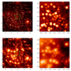 |
Fig. 1. Upper left: deep image after combining all 2012 Ks exposures with the holography technique. Lower left: deep image after combining all 2012 Ks exposures with the SSA technique. The insets on the right hand side show magnifications of the areas marked by the green squares. Colour scales are logarithmic. The axes mark offsets from Sgr A* along Right Ascension and Declination in arcseconds. |
3. Astrometry, photometry, and completeness
3.1. Source detection
We used the StarFinder software for photometry and astrometry (Diolaiti et al. 2000). For the large Ks mosaic we chose a detection threshold of 3σ, with two iterations. StarFinder was run three times, with three different correlation thresholds of 0.60, 0.70, and 0.80, thus resulting in three different lists that reflect the uncertainty of the setting of the correlation threshold value. A spatially variable PSF was used, as described in Gallego-Cano et al. (2018). In particular, the PSF was determined for small 13.8″ × 13.8″ sub-fields. The pattern of sub-fields overlapped by 6.9″. The multiple measurements in the overlap regions were used to estimate the uncertainty introduced by the variable PSF (see also Schödel 2010). The latter uncertainty term is approximately constant for all magnitudes and across the mosaic. It was added in quadrature to the formal uncertainties returned by StarFinder.
A different procedure was applied to the central field, which is the most crowded area and therefore most prone to errors. The central field is small enough to perform computationally intensive work. We used the bootstrapped images to infer astrometric and photometric uncertainties. We proceeded as follows: (1) Run StarFinder on the deep image with three iterations, using a 3σ detection threshold, a minimum correlation coefficient of 0.7, a back_box parameter of eight pixels (it is used to estimate the diffuse background), and applying deblending of very close sources. StarFinder returns a correlation value of −1.0 for extended sources. They were excluded from the list of detected stars. We thus obtained what we call the “master list”. (2) Run StarFinder on the 100 bootstrapped images with the same parameters. (3) Compare the master list with the lists obtained from the bootstrapped images. Sources detected within 0.04″ of a star in the master list are considered to be the same star. (4) Create a final list with stars that are detected in ≥70% of the bootstrapped images. The astrometric and photometric positions and uncertainties are computed from the mean and standard deviation of the measurements in the bootstrapped images, after having corrected for small systematic offsets between the lists from the bootstrapped images and from the deep image.
3.2. Calibration
Astrometric calibration was achieved using the reported positions and proper motions of the maser stars IRS 9, IRS 7 IRS 12N, IRS 28, IRS 17, IRS 10EE, and IRS 15NE (Reid et al. 2007). The uncertainty of the astrometric calibration was estimated by comparing the recovered positions after repeating the alignment procedure, dropping a different one of the maser sources each time. The star IRS 17 showed the greatest standard deviation with about 0.01″. We did not take any optical distortion of the S27 camera into account (e.g. Plewa et al. 2015). However, precision (milli-arcsecond) astrometry is not relevant to the scientific purpose of this paper.
The H-band data were treated in the same way as the Ks-band data and were aligned astrometrically with the latter. Sources coincident within 0.040″ after alignment (with a second order polynomial) were considered to be the same star. For photometric calibration we used the magnitudes of the stars IRS 16C, IRS 16NW, and IRS 33N as reported by Schödel et al. (2010) (Ks = 9.93, 10.14, 11.20, H = 11.90, 12.03, 13.24). The resulting uncertainties of the zero points are 0.06 mag.
Since the field-of-view of the central, 9.72″ × 9.72″ field is smaller than the anisoplanatic patch in the observed band and since we did not notice any significant, systematic residuals in the point-source subtracted images, we did not take into account any potential uncertainties related to small changes of the PSF across the field. The analysis and conclusions of this paper do not require any particularly high precision or accuracy in the photometry and astrometry.
The astrometric and photometric uncertainties for the holography and SSA images technique are compared in Fig. 2. The astrometric and photometric uncertainties for the holographic and SSA techniques are similar, but they are somewhat smaller for the holographic image. The holography procedure is linear and the large number of individual frames makes sure that the division in Fourier space, on which the holographic method is based, does not introduce any significant additional uncertainty. A significantly larger number of faint sources is detected in the holographic image (see below). This is probably the case because the holographic method concentrates the light from the stars into very compact PSFs, which enhances the contrast of the image, particularly near the numerous bright stars in the field.
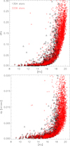 |
Fig. 2. Photometric and astrometric uncertainties in the central, 9.72″ × 9.72″ field. Upper plot: 1σ uncertainty of the measured Ks magnitude of the detected stars plotted over the corresponding Ks magnitude. Lower plot: 1σ relative astrometric uncertainties. Red crosses refer to stars measured in the holographic image. Black triangles mark stars measured in the SSA image. |
3.3. Source lists
Table C.1 lists the positions and magnitudes of the stars detected in the large field with a correlation threshold of 0.70. There are about 39 000 detections at Ks with about 11 000 associated H-band measurements. The final, full source list is available electronically. The 2010 H-band star list and the 2012 Ks-band lists were aligned via a second degree polynomial fit and stars coincident within 0.04″ were considered to be the same source. A proper motion of 1 mas per year corresponds to about 40 km s−1 at the distance of the GC. Therefore, even stars near Sgr A*, moving at several hundreds of km s−1, will be cross-identified by this procedure because the time baseline is only two years.
By following the procedure outlined in the preceding paragraphs, we identified 3336 stars in the holographically treated data and 1304 stars in the SSA image for 2012 in the central field. Almost all the additionally detected stars in the image processed via holography were detected at faint magnitudes. The astrometric and photometric uncertainties were found to be smaller for the holographically treated image than for the SSA image (Fig. 2). Figure 3 shows a comparison of the raw Ks luminosity functions (KLFs) of the SSA and holographic image. Table C.2 lists the positions of the stars relative to Sgr A*, their Ks-magnitudes and uncertainties. The full list is available at the CDS.
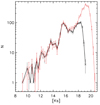 |
Fig. 3. KLF for the stars detected in the holographic image (red) and in the SSA image (black). |
3.4. Completeness
Completeness is usually estimated via the method of artificially inserting stars into images. In the GC observations used here, completeness is mainly limited by stellar crowding. A special problem in the complicated GC field is the challenge to avoid including spurious sources into the final star lists. As already discussed in Gallego-Cano et al. (2018) or Schödel et al. (2014b), the use of noise maps is very efficient in suppressing the detection of spurious sources. In addition to a detection significance of 3σ, in the case of the central field we demand that each accepted source be present in 70% of the bootstrapped images. Spurious sources can thus be efficiently suppressed. Unfortunately, this complex procedure, including many individual exposures, bootstrapped images, and different selection criteria, means that a completeness test via artificial stars would be very complex and extremely time consuming. We therefore resort to an alternative method, as initially described by Eisenhauer et al. (1998) and later applied by Harayama et al. (2008) or Schödel et al. (2010), for example.
In brief, the method is based on an analysis of the distances and magnitude differences between pairs of detected stars. From these data the so-called critical distance can be determined for any given magnitude difference, inside of which the detection probability for a faint star close to a brighter star drops rapidly. For determining the critical radius, one assumes a detection probability threshold, typically 50%. With the set of magnitude differences and critical distances one can build completeness maps. The method is based on some simplifying assumptions, such as a locally approximately constant density of stars of a given magnitude (Here we mean by “local” an area of the order of one to a few square arcseconds). While being less direct than the artificial stars technique, the method of Eisenhauer et al. (1998) has the great advantage that it can be directly applied to lists of stars that result from complex selection procedures. Also, it is computationally far less demanding than the standard method. The inferred completeness fraction for given stellar magnitudes is shown in Fig. 4. The uncertainties were estimated by varying the detection probability threshold between 40% and 60%.
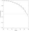 |
Fig. 4. Completeness as a function of stellar magnitude for the central field. The horizontal line indicates 50% completeness due to crowding. |
We find that the 50% completeness limit due to crowding is at Ks ≈ 19.5. This is roughly a magnitude deeper than in our previous work (see Fig. 3 in Gallego-Cano et al. 2018). The latter work was based on the same data, but with a final, deep image obtained via an SSA image. When we analyse the completeness of our SSA image of the central region with the method used here, we obtain a 50% completeness limit of Ks = 18.5.
We also used the above-described procedure to estimate completeness in the large field. The procedure was applied to the three lists obtained with three different values of the StarFinder correlation threshold. We also varied the probability threshold that is used to infer the critical radius between 30% and 70% to infer the related uncertainties, which we found to be smaller than 5 percentage points for the entire considered range of magnitudes. We found that the completeness due to crowding was ≳70% for all sources Ks ≤ 18.5.
Variable extinction may reduce the completeness of faint stars in high-extinction areas. However, deviations from mean extinction in the fields observed by us are generally <0.5 mag (see extinction maps in Schödel et al. 2010). Since the 3σ detection limit of our observations is Ks ≳ 20, but we analyse the luminosity function only down to Ks = 19, we therefore consider completeness due to variable extinction not to be of any concern for this work.
4. Extinction correction and final source selection
Young, massive stars were identified by cross-matching our source lists with the spectroscopically identified young stars found by Do et al. (2009) and Bartko et al. (2009). For estimating interstellar extinction, we excluded foreground stars and highly (probably intrinsically) reddened sources by red and blue colour cuts (H − Ks ≥ 1.4 and H − Ks ≤ 2.5). We additionally limited the source selection to 18 ≤ Ks ≤ 14 as indicated in the upper panel of Fig. 5. In this way we include giants of a mostly homogeneous colour and minimise bias due to very bright giants and also minimise bias due to the incompleteness of the H-band data for faint stars. Subsequently we assumed intrinsic colours of H − Ks = −0.1 for hot, massive stars and H − Ks = 0.1 for all other stars. Due to the very limited range of the intrinsic stellar colours for the chosen filters and potential stellar population this approach is a well-justified approximation (see, e.g. Schödel et al. 2010).
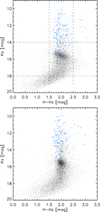 |
Fig. 5. Upper panel: HKs colour magnitude diagram (CMD) for our data (large field). Colour cuts for the creation of the extinction map to exclude foreground stars, highly reddened stars, and faint stars, where the H-band data become incomplete, are indicated by dashed lines. Blue diamonds mark spectroscopically identified young, massive stars. Lower panel: extinction corrected CMD. |
We then estimated the extinction for each star individually from the H − Ks colour excess of all neighbouring stars within a projected radius of 1″. The mean colour excess was determined with the IDL astrolib ROBUST_MEAN procedure in order to exclude any > 3σ outliers. Finally, we assumed for the reddening law Aλ ∝ λ−α, where Aλ is the extinction in magnitude for a given wavelength, λ. We chose α = 2.21 (Schödel et al. 2010; Nogueras-Lara et al. 2018a, 2019a). The typical uncertainties of the derived AK is 0.05 mag. The resulting extinction map is extremely similar to the corresponding part of the extinction map published by Schödel et al. (2010). For this reason we do not show it here. The extinction correction was also applied to stars that were too faint to have an H−band counterpart.
The lower panel of Fig. 5 shows the extinction-corrected CMD, shifted to the mean extinction of the field. The extinction correction reduces visibly the scatter of the data points and the Red Clump (RC) appears like a compact cloud of points centred on Ks ≈ 15.75 and H − Ks ≈ 2.0. Also, the spectroscopically identified young stars (blue diamonds), scatter less after the extinction correction and align approximately along a vertical line to the left of the giant branch, as is to be expected for hot stars. The extinction-correction for foreground stars is overestimated, but they will be excluded from our analysis by the colour cut described in the first paragraph of this section.
5. Ks-Luminosity function
5.1. Large field
The extinction and completeness corrected KLF for the large field with a binning of 0.20 mag is shown in Fig. 6. All stars with colours H − Ks ≥ 1.4 were excluded as foreground stars (see, e.g. Nogueras-Lara et al. 2018a, 2019b, and discussion therein). The KLF is the result of averaging the detections from the three StarFinder runs with different correlation thresholds (see Sect. 3.1) and is shifted to a mean extinction of AKs = 2.62 mag. The uncertainty bars include the Poisson uncertainty (square root of the counts), the uncertainty of the completeness correction, and the uncertainty due to using different correlation threshold parameters in StarFinder (see Appendix A).
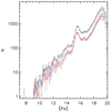 |
Fig. 6. KLF for the large field (black), after exclusion of foreground sources, correction for completeness due to crowding, and correction for differential extinction, assuming a mean extinction of AKs = 2.62. The blue and red lines are the KLFs of the same data, but for the region inside (blue) and outside (red) of a projected radius of 0.5 pc around Sgr A*. The red and blue lines have been scaled by an arbitrary factor to match at Ks > 14. |
Since the faintest stars have higher photometric uncertainties (∼0.3 mag at Ks ≈ 19), they show a significant scatter in colour (see Fig. 5). We considered all stars with H − Ks < 1.4 (roughly two standard deviations from the mean colour) as foreground stars.
The blue and red lines in Fig. 6 show the KLFs for the regions inside (blue) and outside (red) of a projected radius R = 0.5 pc around Sgr A*. At Ks ≤ 14 one can see some systematic excess in the inner half parsec. It is caused by the roughly 200 spectroscopically identified massive young stars located within a projected radius of R = 0.5 pc around Sgr A*. They are strongly concentrated towards the centre (Paumard et al. 2006; Bartko et al. 2009; Lu et al. 2009; Yelda et al. 2014). There is no significant difference between the two KLFs at fainter magnitudes.
5.2. Central field
In Fig. 7 we show a comparison between the KLF of the large field and the one we created from the star list of the holographic image of the central field both corrected for extinction and crowding, foreground stars excluded. There is no significant difference, except for the excess due to young massive stars at Ks ≤ 14 in the central field, as mentioned above. We can see that at the faintest magnitudes the KLF of the central field does not show any deficiencies. This is in spite of the central field suffering extreme crowding and the presence of a high concentration of bright stars, while the number counts of the KLF from the large field are dominated by much larger and less crowded fields. This vindicates the application of the holography technique to the central field.
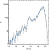 |
Fig. 7. Comparison between the KLF of the large field (blue, scaled by an arbitrary factor to facilitate comparison) and the KLF for the central field (black) (both LFs corrected for differential extinction and for completeness due to crowding, with foreground sources excluded). |
The fact that the KLFs of the central and large regions are indistinguishable after the exclusion of the spectroscopically identified young stars supports strongly the notion that the most recent star formation event near Sgr A* had a top-heavy initial mass function, as analysed and discussed by, e.g. Bartko et al. (2010) and Lu et al. (2013). Gallego-Cano et al. (2018) show how the pre-main sequence stars of this population should show up prominently in the KLF of the central region if the initial mass function had been of standard form. The only caveat of this reasoning is that it does not consider potential mass segregation between the heavier and the lighter stars of the young population.
Potential sources of systematics in the creation of the KLF for the central field are, for example: (1) The acceptance threshold for real stars in the bootstrap procedure, (2) the colour cut, and (3) the inclusion of the crowded IRS 13 area that contains much gas and dust and may give rise to spurious sources or bias the results because it may contain young stellar objects (see, e.g. Mužić et al. 2008; Eckart et al. 2013). Changing the colour cut from H − Ks = 1.4 to 1.6 will make the data points vary well within their 1σ uncertainties. The same is the case for inclusion or exclusion of the IRS 13 area. In order to take the acceptance threshold into account, we computed the mean KLF and its corresponding uncertainties resulting from combining acceptance thresholds of 50%, 70%, and 90%. This is the KLF shown in Fig. 7.
Since the KLFs of the large and of the central fields are indistinguishable within their uncertainties, we only analyse the KLF of the large field in the following sections. The KLF of the large field offers the advantage of smaller statistical uncertainties.
6. Star formation history
The KLF can be used to constrain the star formation history of the MWNSC by comparing it with models created on the basis of theoretical isochrones. While colour-magnitude diagrams are more powerful tools, of course, the intrinsic stellar colours in the two near-infrared bands used in this work are small and the measured colours have uncertainties H − Ks ≳ 0.1 due to measurement uncertainties, potential variability (data are not from the same epoch), and the uncertainty of the extinction correction. Also, since extinction rises steeply towards shorter wavelengths, completeness at H is significantly smaller than at Ks. We therefore use the colour information only for extinction correction, but not for studying the stellar population.
We use combinations of single age stellar populations based on the updated BaSTI isochrones1 (Pietrinferni et al. 2004, 2013; Bedin et al. 2005; Cordier et al. 2007; Hidalgo et al. 2018). The isochrones were computed based on scaled solar metallicities, taking overshooting and diffusion into account, assuming a mass loss coefficient of η = 0.3 and a Helium fraction of 0.247. We used a Salpeter initial mass function (IMF). Given that the range of masses sampled by our observational data is very small (very roughly 1−2 M⊙, with the exception of the youngest stars) the exact IMF used will have very little impact on the results. From the BaSTI models we chose isochrones for metallicities of approximately twice solar ([Fe/H] = 0.30 dex), one and a half times solar ([Fe/H] = 0.15 dex), solar ([Fe/H] = 0.06 dex) and half solar ([Fe/H] = −0.30 dex).
We limit the fits on the bright end of the KLF to Ks ≤ 10.0 because the isochrones used do not extend to include brighter stars, and at its faint end to Ks ≤ 19.0 because of completeness. These magnitudes corresponds to extinction corrected magnitudes 7.4 ≲ Ks ≲ 16.4, where completeness is above 50%. We treat the extinction, AKs as a free parameter. In order to account for photometric uncertainties, uncertainties of the line-of-sight distance, uncertainties in the differential extinction correction of our photometry, and photometric uncertainties intrinsic to the stars (e.g. due to variability of differences in metal content), we include a smoothing parameter in the fits, which is used to smooth the theoretical models with a Gaussian function of FWHM given by this parameter. It is let to vary freely, and is typically of the order one to a few.
6.1. Number of star formation events
An important – and a priori unknown – ingredient in a stellar population model fit to the KLF is the number of the star formation events. In this work we are mainly interested in the question whether stars are old enough to be dynamically relaxed, which implies ages of at least a few Gyr. Since we are not interested in a high precision of the ages of given events (which is very difficult to obtain), we selected the ages that form part of our models after visual inspection of the differences between single age KLFs (see also Nogueras-Lara et al. 2019b). The older the stellar population is, the slower the LF changes with age. We chose the following 16 ages: 13, 11, 9, 7, 6, 5, 4, 3, 2, and 1 Gyr and 800, 500, 250, 150, 100, 80, and 30 Myr. We chose Johnson-Cousins filters for the models. The differences between a Johnson-Cousins K filter and the Ks filter used for the observations can be neglected for the aims of this work.
In a first step we estimated the number of single age populations necessary to provide a good fit to the measured KLF. We fitted all possible combinations of between two to eight theoretical LFs from our initial age selection to the data and plotted the best reduced χ2 against the number of populations, as shown in Fig. 8. All fits with solar and supersolar metallicities reach very similarly low levels of reduced χ2 with just five populations of different ages. Reduced χ2 values for half solar metallicity are consistently higher than for the higher metallicities. The best fit solutions were searched for with the IDL MPFIT package (Markwardt et al. 2009). We set the initial weight of all populations to zero except for the two oldest populations that were assigned ten different initial random values, with the best solution given by the lowest achieved χ2. We assured through extensive tests (using thousands of random initial values, assigning random or constant initial weights) that with this setup the best-fit solutions were robust and did not correspond to local minima.
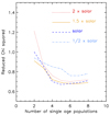 |
Fig. 8. Minimum reduced χ2 plotted against number of single age stellar populations that are used to fit the measured KLF. |
In Fig. 9 we show the SFH for assuming five single age star forming events and for metallicities of 0.5, 1, 1.5, and 2 times solar. In all cases, >50% of the original stellar mass formed ≳10 Gyr ago. In the solar metallicity model about 40% of the stellar mass may have formed at intermediate (3–4 Gyr) ages. Spectroscopic studies indicate that about 80% of the stellar mass formed more than 5 Gyr ago (Blum et al. 2003; Pfuhl et al. 2011) and that the mean metallicity in the NSC is super-solar (Do et al. 2015; Schultheis et al. 2019). Therefore, we prefer the models with 1.5 to 2 times solar metallicity.
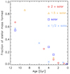 |
Fig. 9. Star formation histories for five single age events with different mean metallicities. Not all data points can be clearly seen because they bunch together at young ages. |
6.2. Fits with many populations
Next, we determined the best fit solution by allowing a combination made up of all 16 single age populations for which we had calculated the KLF. We set the initial weight of all populations to zero except for the five oldest populations that were assigned one thousand different initial random values. We ensured by extensive tests that we could find the global χ2 minimum successfully with this approach. Table 2 gives the values of the parameters for the best fits for the models with mean metallicities of 0.5, 1.0, 1.5, and 2 times solar as well as for a model with a mixture of metallicities for the three oldest ages (20% for 0.5, 20% for 1, 30% for 1.5, and 30% for 2 times solar). The resulting best-fit parameters for the latter are close to the case of 1.5 times solar metallicity, as expected. This test served to verify the validity of our approach to fit mean metallicity models to a stellar population that contains in reality a range of different metallicities. The top panel of Fig. 10 shows the best fit for the 1.5 solar metallicity case, that results in the overall lowest χ2. The formal uncertainties of the parameters are not listed in the table. They are generally large because of the degeneracy of the high similarity of KLFs between adjacent age bins.
Best model fits to the KLF, considering stellar populations of 16 different ages and different metallicities.
While binned data have the advantage of being easier to interpret, the binning may impose a loss of information or additional uncertainty. We therefore also performed fits on cumulative KLFs. The resulting best-fit parameters are listed in Table 3. The bottom panel of Fig. 10 shows the fit of the cumulative KLF for [Fe/H] = 1.5 solar. The fits to the cumulative LF are more stable to initial conditions and are more consistent in the derived SFH for different metallicities. Therefore, in the following part of this work, we focus on the results from fits to the cumulative KLF from this point on.
Best model fits to the cumulative KLF, considering stellar populations of 16 different ages and different metallicities, with and without spectroscopically confirmed young stars.
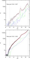 |
Fig. 10. Top: best fit of the KLF (foreground sources excluded, corrected for differential extinction and for completeness due to crowding) with 16 single age populations for 1.5 times solar [Fe/H] (Col. 4 in Table 2). Violet: 13, 11, 9, 7 Gyr; green: 2 and 3 Gyr; blue: ≲0.5 Gyr. Bottom: same, but for the cumulative KLF (Col. 4 in Table 3). |
6.3. Systematics
There are many potential sources of systematic uncertainty in the stellar population fits. In this section we examine the ones that we could identify and considered possibly significant. By using the cumulative LFs we can already eliminate binning as a possible source of systematics. Other sources are:
1. Foreground stars, IRS 13. Systematic effects may result from our choice of threshold for exclusion of foreground stars and from the inclusion or exclusion of the potential cluster IRS 13 (e.g. Schödel et al. 2005; Fritz et al. 2010), We created the KLF of the large field with a stricter criterion for the exclusion of foreground stars (H − Ks < 1.7). The resulting KLF is indistinguishable, within the errors, from the one used in the analysis above. The inclusion or exclusion of sources from the IRS 13 region into the KLF did not have any significant effect.
2. Spectroscopically identified massive, young stars. It is well established that there is a few million year old population of massive young stars present within a projected distance of 0.5 pc from Sgr A*. The properties and formation of these stars are still a topic of intense investigation. There is now strong evidence that the corresponding starburst must have had a top-heavy initial mass function (Nayakshin & Sunyaev 2005; Bartko et al. 2010; Pfuhl et al. 2011; Lu et al. 2013). This means that the contamination of the KLF by lower-mass young stars from this event, which have not been spectroscopically identified, is probably minor (see Fig. 12 in Gallego-Cano et al. 2018). Evidence for this latter point is also provided by our comparison of the KLFs inside and outside a projected radius of R = 0.5 pc from Sgr A*, as shown in Fig. 6. In our modelling we have not included any population of stars in the corresponding age range, in particular because BaSTI models do not extend to such young ages. We therefore cleaned the LFs from the spectroscopically identified young, massive stars. The resulting best-fit parameters are listed in the columns after Col. 5 in Table 3. The reduced χ2 values become somewhat smaller and super-solar metallicities become somewhat more favoured. The general SFH is not changed. We conclude that the presence of young, massive stars does not introduce any strong bias, but that it is better to remove those stars from the sample. From here on, we therefore only use LFs without the spectroscopically identified young, massive stars.
3. Initial mass function. We used a Salpeter IMF, that is, an exponential IMF with an exponent of −2.35. Our data are dominated by giants which cover a very narrow mass range, (e.g. 0.7−1.7 M⊙ for 2 Gyr age, 0.7−1.1 M⊙ for 9 Gyr age). Therefore there is little leverage to measure the IMF. Also, the SFH study by Pfuhl et al. (2011) finds that a Chabrier/Kroupa IMF (very similar to a Salpeter IMF at masses above one solar mass) works well on the central parsec, except for the already discussed case of the young, massive stars. We tested the assumptions on the IMF by fitting the cumulative KLF with BaSTI isochrones with a top-heavy IMF with an exponent of −1.7. The resulting SFH is detailed in Col. 9 of Table 3. Within the uncertainties it is indistinguishable from the one derived assuming a Salpeter IMF.
4. Fitting range. In order to test the importance of the faint magnitude cut-off used to fit the cumulative KLF – for example because of potential completeness variation due to spatially variable extinction –, we performed fits with cut-offs at Ks = 18.75 and at Ks = 19.25 instead of at Ks = 19. The resulting SFHs are listed in Cols. 10 and 11 of Table 3. The brighter cut-off results in a somewhat stronger contribution appearing at 3 Gyr, while the fainter cut-off will increase the weight of the oldest population and shift the age of the 3 Gyr population a bit towards 4 Gyr. The changes are not substantial and reflect the fact that the oldest population are traced best by the increase of star counts at the faintest magnitudes.
5. Metallicity. Most spectroscopic studies in the past decades found solar to supersolar mean metallicities at the GC (Ramírez et al. 2000; Cunha et al. 2007; Do et al. 2015; Feldmeier-Krause et al. 2017b; Nandakumar et al. 2018). Some studies found somewhat lower mean metallicities (Rich et al. 2017). The meta-study by Schultheis et al. (2019) argues that the metallicity distribution in the innermost bulge is complex, but that the GC has a high supersolar mean metallicity with [Fe/H] = +0.2 dex. We note that the latter study uses GC sample of Nandakumar et al. (2018), who did not find any stars with sub-solar metallicity in the proper GC field. Finally, the photometric study by Nogueras-Lara et al. (2018b) of the innermost bulge, at projected distances of 60−90 pc to Galactic north from Sgr A*, indicates a single-age stellar population of twice solar metallicity. In conclusion, current evidence points towards solar to super-solar mean metallicity in the nuclear star cluster.
The stellar population fits to the KLFs performed here, are consistent with the spectroscopic results, as can be seen in Fig. 8 and Table 3. We note that exclusion of the spectroscopically identified massive stars improves the χ2 of the fit with supersolar metallicities, but not for the one with solar mean metallicity. A mean metallicity of half solar for all ages can be excluded with high confidence and the overall best fit is achieved for a metallicity of [Fe/H] = +0.2 dex, after exclusion of the spectroscopically identified young stars. Finally, we have performed a population fit in which we assign half solar metallicity only to the oldest two age bins (13 and 11 Gyr). The result is shown in the last column of Table 3: reduced χ2 is higher than for all other cases except the one when all populations are forced to have low metallicity. In fact, the weights of the low metallicity populations result to be zero, which is equivalent to limiting the age of the stars in the cluster. At the same time the best-fit smoothing factor is higher than in all other cases. We conclude that setting the oldest populations to a low metallicity does not lead to a satisfactory fit. To conclude, as concerns metallicity, the inferred star formation history is robust with respect to the assumed mean metallicity in the range one to two times solar [Fe/H].
6. Stellar evolutionary codes. We also fitted the data with theoretical cumulative KLFs based on two other stellar evolution codes: PARSEC (release v1.2S + COLIBRI S_35 Bressan et al. 2012; Chen et al. 2014, 2015; Tang et al. 2014; Marigo et al. 2017; Pastorelli et al. 2019) and MIST (Dotter 2016; Choi et al. 2016; Paxton et al. 2011, 2013, 2015). We used scaled solar metallicities. The parameters of the best fits are listed in Tables D.1 and D.2. We note:
– The achieved minimum χ2 values are worse for PARSEC and MIST than for BaSTI. More importantly, while for BaSTI the minimum χ2 values decrease further when we exclude the spectroscopically young, massive stars from the data, as is expected because our models do not contain sufficiently young isochrones, the χ2 values actually increase in this case for MIST and PARSEC to about twice the minimum values reached in BaSTI. It appears that the most recent release of BaSTI (Hidalgo et al. 2018) is suited better for the GC stellar populations than the other two models.
– Independent of metallicity and whether the young massive stars are excluded or included, all SFHs derived with PARSEC imply that ≳40% of stars formed 5 Gyr or less ago. This result contradicts constraints from spectroscopic studies, which require the stellar mass formed at these ages to be ≲20% (Blum et al. 2003; Pfuhl et al. 2011).
– The SFH inferred with MIST isochrones after exclusion of spectroscopically identified massive, young stars agrees for solar and 1.5 solar [Fe/H] – in spite of the high χ2 values – reasonably well with the SFH from BaSTI isochrones at these metallicities. The main difference is that the stellar mass formed at intermediate ages is concentrated at 3 Gyr in the BaSTI fits and split between 4 and 2 Gyr in the MIST fits. Some age shifts between the models are expected (see also the comparison of MIST and BaSTI LFs discussed in the appendix of Nogueras-Lara et al. 2019b).
Conclusion. The systematic effects studied here show that the mean metallicity of the NSC appears to be solar to super solar, with only small differences in the derived SFH. In agreement with spectroscopic studies, sub-solar mean metallicity appears to be highly unlikely. After excluding fits with PARSEC isochrones on the basis that they do not agree with the mentioned spectroscopic findings and do not agree with the fits based on MIST or BaSTI isochrones, we conclude that none of the examined systematics alters the derived SFH significantly.
6.4. Monte Carlo simulation
To further explore uncertainties, we created 10 000 realisations of the cumulative KLF in a Monte Carlo (MC) simulation, based on the mean and standard deviation in each magnitude bin, and fitted those random cumulative KLFs again with a combination of 16 different populations. Spectroscopically confirmed massive, young stars were excluded. The fits were performed for mean [Fe/H] of 1.0, 2.0, and 1.5 times solar. The lowest reduced χ2 values were achieved for [Fe/H] = 2.0 solar in 26% of the cases, for [Fe/H] = 1.5 solar in 74% of the cases, and for [Fe/H] = 1.0 solar in 0% of the cases, indicating a preference for super solar mean metallicity of roughly +0.2 dex, in agreement with the spectroscopic analysis by Schultheis et al. (2019). Figure 11 show histograms of the relative contributions of the different ages for a mean metallicity of 1.5 times solar [Fe/H]. We show the corresponding plot for BaSTI isochrones and solar metallicity and for MIST isochrones and 1.5 times solar metallicity in Appendix B, too. They show broader, less well defined distributions, but agree well with Fig. 11 in general. In Appendix B we also show histograms of the reduced χ2 values for the MC fits with BaSTI isochrones and different mean metallicities.
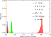 |
Fig. 11. Histograms of the stellar mass fraction formed in given age ranges derived from fits to MC simulations of the cumulative KLF with BaSTI isochrones and assuming a mean [Fe/H] of 1.5 times solar. |
6.5. Conclusions on the star formation history
Star formation history: After having examined systematics and having performed the MC simulations, a clear picture of the formation history of the MWNSC emerges:
1. About 80% or of the star formation occurred > 10 Gyr ago.
2. Very little activity occurred between 5 and 10 Gyr ago, where at most 5%, but probably close to 0% of star formation occurred.
3. There is clear evidence for an intermediate age population of 2−4 Gyr, which contributes around 15% of star formation.
4. A clear minimum existed at around 1 Gyr.
5. Finally, a few percent of the nuclear cluster’s mass formed in the past 150–500 Myr.
6. ≲1% of star formation happened in the past 100 Myr, with the caveat that our models do not include populations younger than 30 Myr and that the spectroscopically confirmed stars pertaining to the youngest star formation event were excluded from the fits.
7. Stellar density near Sgr A*
We used the high quality central field data to infer the profile of the stellar surface number density within 5″, or 0.2 pc, of Sgr A*. The aim is to look for the signature of a relaxed stellar cusp, which can only be traced by stars old enough to have undergone dynamical relaxation. Since stars at different mean magnitudes can have different mean ages, we plot the analysis for different magnitude bins (Fig. 12). Extinction and completeness correction were applied and spectroscopically identified young hot stars were excluded. Power laws were fitted to the data points. The different power-law indices are listed in Table 4.
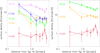 |
Fig. 12. Projected stellar surface density in the deep field. Left: one-magnitude wide bins. Right: two-magnitude wide bins (the brightest bin contains all stars Ks < 15. The dashed lines show simple power-law fits. |
Power-law index α of a single power-law fitted to the projected surface density of stars around Sgr A* in one-magnitude wide brightness bins.
All stars in magnitude bins fainter than Ks = 15 show a density increase towards Sgr A* that can be approximated by a power-law. The power-law indices are consistent with each other within the uncertainties. Stars in the brightest bin do not show this increase, but are rather consistent with a constant, or even decreasing, surface density. The stellar surface densities presented here reach about 0.5 mag deeper than the ones presented in Gallego-Cano et al. (2018).
8. Discussion
8.1. Stellar population and formation history
The photometric measurements for > 30 000 stars, combined with extinction measurements with an angular resolution around 1″, allow us to present the so far deepest and most detailed KLF of the Milky Way’s NSC.
An important fundamental question is the approximate distance depth of the data, that determines which stellar structure dominates our sample. As concerns stars in the Galactic foreground, located in spiral arms or in the bar/bulge in front of the central molecular zone, they can be reliably excluded by their blue colours as we do in this work and as can be seen in the detailed colour magnitude diagrams presented in previous work (see, e.g., Schödel et al. 2010; Nogueras-Lara et al. 2019c). It is less straightforward to assess the contribution from background stars. However, a look at the surface density of stars in the GC region can help. The surface flux and number density as a projected function from Sgr A* show that the projected stellar density within a projected radius R ≲ 1 pc is at least five times higher than at R ≳ 5 pc because of the steep increase of stellar density towards the cusp of the Milky Way’s nuclear star cluster (e.g. Schödel et al. 2014a; Gallego-Cano et al. 2018). Therefore, we assume here that our KLF is dominated by stars inside the central few parsecs of the MWNSC, with a contamination of not more than about 10% of stars in the fore- and background of the cluster. Also, our observation of an indistinguishable KLF between the very central parts of the MWNSC (R < 0.5 pc) and the parts at somewhat greater R, as shown in Sect. 5.2 supports our assumption that our sample is dominated by stars within a few parsecs around Sgr A*.
The KLF appears to be well mixed and shows hardly any kind of dependence on distance from Sgr A*. There is some excess in the numbers of stars brighter than Ks ≈ 14.5 at projected distances R < 12.5″/0.5 pc from Sgr A* due to the presence of young, massive stars, but this excess is small. At magnitudes Ks > 15 the KLF in the centralmost arcseconds is identical, within the uncertainties, to the one at distances of R = 25″/1 pc. The stellar population therefore appears to be homogeneous and we can analyse the SFH history by using the KLF of the entire field.
Because of the sensitivity of our data we detect an upturn of the KLF at Ks > 18. While previous, shallower KLFs, as presented in Genzel et al. (2003), Schödel et al. (2007), or Pfuhl et al. (2011), were consistent with an old, bulge-like stellar population with an admixture of young stars, the KLF presented here requires the presence of intermediate-age stars of ages 2–4 Gyr.
This is the first time that a detailed SFH of the MWNSC has been inferred from its KLF. Although the KLF of the MWNSC is included in the data of Figer et al. (2004) it is not discussed separately there. Other publications, e.g. Genzel et al. (2003) and Schödel et al. (2010) present KLFs for the central parsec of the GC, but the KLFs are shallower and less detailed. Also, they do not discuss the SFH apart from noting that the KLF is consistent with an old, bulge-like population. The deep, carefully extinction-corrected KLF presented here contains features that are sensitive to the SFH. Those are: (1) The number of stars brighter than the AGB are sensitive to recently formed massive stars, (2) the relative weights and distances between the RC and the RGBB (Red Giant Branch Bump) are sensitive to age and metallicity of stars older than a few Gyr (RC and RGBB are not individually resolved in our KLF but are mixed together in the RC bump), (3) the upturn of the KLF at magnitudes fainter than the RGBB (intermediate age stars), and (4) the number counts in the region between the upturn of the KLF and the RC/RGBB bumps (young stars). Finally through the use of the cumulative KLF we can minimise potential systematic effects due to the choice of the bin size in the differential KLF.
After investigating the possible systematics, the following general picture emerges: (1) About 80 ± 5% of originally formed stellar mass formed very early in the Milky Way’s history. In all cases the model LFs fitted to the data prefer ages of 13 Gyr. We are certain that such an old age must be interpreted with certain caution given that stellar evolutionary models may give rise to ambiguities at such old ages and high metallicities, where they cannot be calibrated well. We therefore believe that it may be safe to say that ∼80% of the original cluster mass formed at least about 10 Gyr ago. (2) Very little star formation occurred at intermediate-old ages of 5–9 Gyr, at most a few percent, with zero being the most likely scenario. (3) Star formation clearly occurred at intermediate-young ages of 2–4 Gyr, when roughly 15% of the originally created stellar mass formed. The age uncertainty is largely model-dependent. If we rely on any given evolutionary track then this star formation event appears to be clearly placed in time, for example 3.0 ± 0.5 Gyr when relying on BaSTI isochrones. (4) Star formation activity was close to zero about 1 Gyr ago (see Table 2). (5) Finally, there is evidence of star formation in the past few 100 Myr and in the recent past (< 100 Myr ago), although we cannot pinpoint the exact ages. About 1% of the stars formed in the past 100 Myr, and of the order 3% between 150 and 500 Myr ago. Our elaborate multi-population fitting therefore confirms that the star formation history of the NSC can be fitted well with a small number of star formation events: One at ≳10 Gyr, one at ∼3 Gyr and about 3 at 0–500 Myr, as shown in Sect. 6.1 (see Fig. 8). More star formation events are needed at young ages because of the rapid evolution of the KLF of at ages younger than about 1 Gyr.
The SFH derived here agrees well with the most recent spectroscopic determination of the SFH by Pfuhl et al. (2011) or with previous work by Blum et al. (2003). Those publications found that of the order 70–80% of the stars in the NSC formed more than 5 Gyr ago. We note, however, that: (a) Our work on the KLF has pushed back the age of the NSC considerably because of the sensitivity of the KLF to the onset of the main sequence of old stellar populations. (b) It appears that there was just a single star formation period at intermediate age, around 3 Gyr. We can also confirm the global star formation minimum that Pfuhl et al. (2011) found for ages ∼1 Gyr.
In Fig. 13, we present the star formation rate on a linear scale, by dividing the stellar mass fractions formed in a given time by the approximate length of the time interval. For the latter we assumed 3 Gyr for the oldest event, 5 Gyr for the quiescent time 5–9 Gyr ago, 1 Gyr for the intermediate age stars and correspondingly shorter (and better defined) time intervals for younger events. In agreement with the SFR derived from spectroscopic work by Pfuhl et al. (2011) we see that the star formation rate decreased until 1 Gyr ago but then increased again. Contrary to the model presented in Pfuhl et al. (2011) we find a long minimum of the SFR at ages roughly 5–9 Gyr ago. For modelling purposes the SFH of the NSC can be simply reproduced by assuming five different bursts of star formation. Minima similar to the one observed at ∼1 Gyr may have occurred at other times because star formation will probably not have been homogeneous in time and have proceeded in bursts separated by tens or hundreds of millions of years. The one at 0.8–1 Gyr can, however, be easily detected because the RC magnitude shows a very clear minimum brightness at ages around 1 Gyr that lasts for at most a few 100 Myrs (Girardi 2016). Combined with the large number of stars in the RC, we would be very sensitive to any star formation event that occurred about 1 Gyr ago.
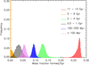 |
Fig. 13. Relative star formation rate in the NSC as a function of time. Histograms corresponding to the SFH from the lower panel of Fig. 11 divided by the approximate length of the corresponding time intervals. |
Our SFH fits prefer high metallicities. This agrees with the most recent spectroscopic analyses (Schultheis et al. 2019). Hence, the assumption of supersolar metallicity of NSC appears to be correct.
8.2. Stellar cusp around Sgr A*
The presence of a density cusp around Sgr A* is expected for stars older than the dynamical relaxation time. Relaxation by two-body effects takes of the order 10 Gyr in the NSC, but several effects, such as the presence of massive perturbers or mass segregation can speed this process up significantly (Perets et al. 2007; Preto & Amaro-Seoane 2010; Alexander 2017). It appears therefore reasonable to assume that stars older than a few Gyr are dynamically relaxed at the GC. The expected stellar cusp is not observed for bright giants, but has been confirmed to be present for stars fainter than Ks ≈ 15.5 (Yusef-Zadeh et al. 2012; Gallego-Cano et al. 2018; Schödel et al. 2018; Habibi et al. 2019). Here we present even deeper star counts than in Gallego-Cano et al. (2018) and confirm that the cusp is consistently detected in the form of a power-law increase of the stellar surface density towards Sgr A*.
While the evidence for a stellar cusp is now strong, its exact properties remain elusive. All tracer stars (even the ones creating the diffuse, unresolved light) are confined to narrow mass intervals. With BaSTI models and at the distance and extinction (assuming AK = 2.5 mag) of the GC all stars of brightness 19 ≲ K < 10 are confined to the narrow mass interval of 1.05−1.10 M⊙ at 11 Gyr age and to 1.45−1.55 M⊙ at 3 Gyr age (see also Baumgardt et al. 2018; Schödel et al. 2018) and should therefore show the profile of a classical Bahcall-Wolf cusp with a power-law exponent of γ = −1.5 for the 3D stellar density (Bahcall & Wolf 1976; Alexander 2017). The projected densities found here and in the above cited publications are mostly flatter than what would be expected for this value. In particular when the 2D data are de-projected, then relatively the power-law exponent takes on relatively small values (as low as γ = −1.1, see Schödel et al. 2018).
Apart from possible systematic effects, in particular when de-projecting the data, a decisively limiting factor in our analyses is the unknown age of individual stars. Aharon & Perets (2015) and Baumgardt et al. (2018) have shown how repeated star formation can create a cusp that is flatter than the classical Bahcall-Wolf cusp, which is based on the simplifying assumptions of a single-age, single-mass, old, dynamically relaxed population. To properly investigate the shape of the cusp, we would need to know the age of the tracer stars. This requires careful spectro-photometric work. Also, currently, efficient spectroscopy is limited to giants brighter than Ks ≈ 16 and to small fields due to the small fields-of-view of adaptive optics assisted integral field spectrographs. The work of Habibi et al. (2019) presents a first step into this direction, but a more global and detailed study of all spectro-photometric data (including a complex completeness analysis) is necessary to address this problem. Alternatively, we may wait for the advent of Extremely-Large-Telescopes to solve this question.
Gallego-Cano et al. (2018) presented a plot of the observable fraction of stars at a given magnitude that is older than 3 Gyr (their Fig. 11). Here, we present a similar plot, based on the MC simulation from Sect. 6.4. In Fig. 14 we show the fraction of stars older than 10 Gyr, along with confidence intervales. As concerns a comparison of this plot with the one shown in Gallego-Cano et al. (2018), the fraction of old stars is lower because the latter was based on the SFH derived by Pfuhl et al. (2011) and considered stars older than 3 Gyr. In our newly derived SFH we find no relevant star formation at ages 5–9 Gyr. This implies an overall higher contamination by young, dynamically unrelaxed stars at magnitudes brighter than K ≈ 20.
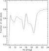 |
Fig. 14. Fraction of observed stars older than 10 Gyr as a function of magnitude at the GC, based on the MC modelling of the data with BaSTI models and mean [Fe/H] of 1.5 solar (corresponding to the SFH shown in Fig. 11). The lines correspond to cumulative probabilities of the simulations: 5% or less of the MC runs (blue dotted), 50% or less of the MC runs (black solid), 95% or less of the MC runs (red dotted). |
We can see the fraction of old, dynamically relaxed stars among the currently observable ones is only around 60% at most magnitudes. Potential contamination by young stars is lowest at the peak of the RC, at K ≈ 16, and highest at K ≈ 19. Consequently, it is not straightforward to compare the observations to the theoretical predictions, in particular quantitatively. With next generation AO instruments and/or extremely large telescopes we will be able to probe the old main sequence stars at K ≳ 20 and thus derive a much clearer picture of the cusp around Sgr A*.
8.3. Stellar remnants
Pulsars in the GC are of great interest because they can serve as exquisite probes of General Relativity if they are located in a tight orbit around Sgr A* or, alternatively, form a binary with a stellar mass black hole (e.g. Eatough et al. 2015). We find that not more than about 1% of the NSC may have formed less than 100 Myr ago. Stars with masses between about 8 to 25 M⊙ that formed during this time may have given rise to still active pulsars (assuming a 100 Myr death line due to spin-down). As a very rough estimate, assuming conservatively that all these young stars formed within 1 pc of Sgr A* and that there are 1 × 10⁶M⊙ of stellar mass within 1 pc of Sgr A*, this results in ∼100 pulsars, assuming a Salpeter IMF and a lower mass cut-off of 0.5 M⊙. This number is not very sensitive to changes in the slope of the IMF: While a more top heavy IMF will produce more massive stars, it will also produce less stars in the mass interval where they end up in neutron stars. However, a lower mass cut-off of the IMF can change this number. For example, for a lower mass cut off of 1 (2) M⊙, the number of expected pulsars increases by a factor of 3 (7).
Of the order 20% of these pulsars could be beamed towards Earth (Eatough et al. 2015). Indeed, a magnetar was detected at 0.1 pc projected distance from Sgr A* (Rea et al. 2013). However, given the small number of expected pulsars, it is highly unlikely that any normal pulsar may be detected that is on a tight orbit around Sgr A* and is beamed towards Earth. Previous estimates of up to 1000 pulsars on short-period (< 100 yr) orbits around Sgr A* appear to be significant overestimations (Pfahl & Loeb 2004). The search for so-called “recycled” pulsars, milli-second pulsars spun up by accretion onto old neutron stars, may be more promising (Eatough et al. 2015).
As concerns the predicted cusp of stellar mass black holes around Sgr A*, stellar mass black holes constitute the heaviest long-lived constituents of the stellar cluster they will mass-segregate towards the central black hole and form a steep cusp around it, which may also be termed dark cluster (see Alexander 2017, and references therein). The existence of a stellar cusp around Sgr A* suggests that stellar cusps and thus dark clusters exist around similar massive black holes in the Universe. In this case, future space-borne gravitational wave observatories will probably detect a significant rate of so-called extreme mass ratio inspiral events (EMRIs, see Amaro-Seoane et al. 2007, and references therein). In simulations, stellar mass black holes are typically assigned masses of 10 M⊙. The higher the metallicity of a star, the more mass it looses via stellar winds during its post-main sequence evolution. This will result in smaller remnant masses. The stellar mass black holes formed in the high-metallicity NSC may therefore have preferentially of the order 6 M⊙ for solar metallicity, and even less for supersolar metallicity precursors (e.g. Banerjee et al. 2020). This may slow down mass segregation and result in a somewhat less steep cusp of the dark cluster.
8.4. Formation of the MWNSC
The two basic formation scenarios suggested for NSCs are globular cluster infall and merger or in-situ growth by star formation within the cluster or accretion of star clusters formed in its vicinity (Böker et al. 2010; Neumayer et al. 2020). In case of the Milky Way, there is direct evidence for the in-situ growth scenario from the observation of young, massive stars close to Sgr A* (see review by Genzel et al. 2010).
If globular clusters were the precursors of a significant fraction of the MWNSC’s mass, we would expect that a very old, sub-solar metallicity population made up a large fraction of its mass. The fact that no RR Lyrae stars have been discovered in the central few parsecs (or at most a single one) points towards a very small fraction of such an old, metal poor population (Dong et al. 2017). This agrees well with the spectroscopic observations by Do et al. (2015) and Feldmeier-Krause et al. (2017b, 2020), who find only of the order 5% of stars with metallicity of half solar or less. Recent spectroscopic studies (Schultheis et al. 2019) and the photometric analysis in this work support a supersolar mean metallicity. The catalogue by Harris (2010) lists 152 Milky Way globular clusters with valid metallicity measurements. There are only five globular clusters with a metallicity > − 0.3 dex and 97% of the clusters in the sample have a lower metallicity. All these observations therefore disfavour globular clusters, such as they are observed today in the Milky Way halo, as MWNSC precursors.
The new SFH of the MWNSC derived in this work appears to push back its original formation to a time ∼10 Gyr ago, when the Milky Way may have suffered its last major mergers (Wyse et al. 2001; Helmi et al. 2018). Such mergers are efficient in funnelling gas to galaxy centres and can thus lead to growth of nuclear star clusters and massive black holes. Dense, metal rich star clusters may have formed closed to the Galactic centre and then have merged to form the MWNSC. By forming originally in dense clusters close to the centre but not in accretion discs around the central black hole, the IMFs of these cluster may have avoided to be strongly top-heavy or bottom-truncated IMF as it has been observed for the youngest stars within 0.5 pc of Sgr A*, which may have formed in such an accretion disc (see Bartko et al. 2010; Genzel et al. 2010; Lu et al. 2013). The IMF of the NSC can therefore be close to standard, as is also suggested by observational work (Löckmann et al. 2010), even though the newest batch of stars has a top-heavy IMF.
8.5. Comparison to SFH of nuclear disc
The SFH of the nuclear stellar disc, that surrounds the MWNSC, has recently been published by Nogueras-Lara et al. (2019b). They find that 80%–90% of the stellar mass in the NSD formed over 8 Gyr ago, followed by a long minimum in activity that was ended by a starburst like event about 1 Gyr ago. They also find increased star formation activity in the past few 100 Myr. The general old age and the high activity in the recent past are consistent with the star formation history of the MWNSC as derived here. There are two notable differences: (1) Nogueras-Lara et al. (2019b) do not report any star forming activity in the nuclear disc at intermediate ages, contrary to the very clear signs of an about 3 Gyr old population that we find in the MWNSC. Either the latter event was limited by some mechanisms to the MWNSC or it was missed in the study of Nogueras-Lara et al. (2019b) because their data are of lower angular resolution and therefore limited by crowding to magnitudes ≲17. The intermediate age population manifests itself in the form of an upturn of the KLF at K > 17.5 (see Fig. 10). (2) The star burst event about 1 Gyr ago found by Nogueras-Lara et al. (2019b) in the NSD does not have any counterpart in the MWNSC. It may have been limited to the NSD with too little gas reaching the MWNSC.
9. Summary and conclusions
We present a new photometric analysis of the Milky Way’s nuclear star cluster in a region within about 1 pc in projection around the massive black hole Sgr A*. The stacked high-quality images result in a star list for what we call the large field here, containing 39 000 Ks magnitudes, which is complemented by 11 000 H measurements. The smaller number of H-band data points is caused by the significantly higher extinction in H and by the availability of less high quality images in that band. In addition, we provide a deep image of a small region of about 10″ × 10″ that results from stacking the AO images with the speckle holography technique. The latter leads to a narrow, Gaussian PSF across the entire image and compensates the relative changes of the PSF across the individual exposures. Applying the speckle holography technique to the AO data significantly reduces incompleteness due to crowding and results in about 50% more stars detected at faint magnitudes as compared to the classical shift-and-add technique. We also provide the source list of the ∼3000 stars detected at Ks in this so-called deep field.
An analysis of the sensitive, extinction and completeness corrected KLF obtained from our data shows that there is no detectable dependence of the KLF on distance from Sgr A*. The only exception is a slightly increased number of stars at Ks = 12−14 within a projected distance of 0.5 pc from Sgr A*, which is due to the young, massive stars present in this region. The super-exponential increase of the KLF at faint magnitudes is evidence for the presence of intermediate age stars (2–4 Gyr), while its high level on the faint side of the Red Clump bump provides evidence for the presence of young (less than a few 100 Myr) stars.
We derive new constraints on the star formation history (SFH) of the NSC from the KLF. A large fraction (∼80%) of the stars formed ≳10 Gyr ago, followed by almost zero activity during more than 5 Gyr. Significant star formation occurred then again ∼3 Gyr ago, when roughly 15% of the original stellar mass were formed. There was a clear minimum in star formation around 0.8–1 Gyr ago and a few percent of the mass formed in the past few 100 Myr. This is not consistent with a quasi-continuous SFH as hypothesised by Morris & Serabyn (1996). The spectroscopic and photometric data can be fit with a simple model, where most of the MWNSC formed ∼10 Gyr ago, with additional star formation at ∼3 Gyr and in the recent past (100 Myr ago to present).
We use the data from the central holographic image to probe for the existence of the predicted stellar cusp at the faintest magnitudes studied via star counts yet. Consistent with previous work we find evidence for a power-law increase of the stellar surface density at all magnitudes fainter than Ks ≈ 15. Brighter giants show a flat profile in the inner ∼5″/0.2 pc. With the help of our analysis of the SFH history we show that the fraction of dynamically relaxed stars (here assumed to be older than about 10 Gyr), which are adequate tracers of the cusp, appears not be much higher than 60% at the observed magnitudes. This means that contamination of the star counts by younger, dynamically unrelaxed stars can be significant at all magnitudes. While the detection of similar power-law profiles at all magnitude bins and even in the faint, unresolved light strongly support the existence of a stellar cusp, the potentially high contamination makes it difficult to infer its properties accurately.
From the SFH we argue that the detection of normal pulsars in tight (< 100 year period) orbits around Sgr A* is unlikely. The high mean metallicity of the MWNSC may imply stellar black hole masses significantly smaller than the typically assumed 10 M⊙.
The high mean metallicity of the MWNSC and its star formation history, which may be quasi-continuous, argue against the hypothesis that globular clusters – such as they are observed in the Milky Way’s halo – have contributed a significant amount of the mass of the MWNSC. However, the MWNSC may have formed from metal-rich dense clusters that formed near the Galactic Centre after gas infall in a major merger.
Further progress in the field can be achieved by studying the stellar density profile using a carefully calibrated sample of stars age-dated via spectrophotometry. Improved instrumentation for AO near-infrared imaging (perhaps the upcoming ERIS at the ESO VLT) may allow us to probe deeper into the faint end of the KLF and thus to obtain better constraints on the relative contributions from the oldest and intermediate-old populations. Adding mid-infrared photometry from the James-Webb-Space Telescope will finally allow us to break the degeneracy between reddening and intrinsic stellar colours and use colour-magnitude diagrams as diagnostics for the formation history of the MWNSC. The superb capabilities of spectroscopic and imaging instrumentation (MOSAIC, HARMONI) at the ESO ELT (Extremely Large Telescope) will probably finally enable us to unambiguously infer the properties of the stellar cusp around Sgr A* and to determine the SFH of the NSC in detail.
Acknowledgments
The research leading to these results has received funding from the European Research Council under the European Union’s Seventh Framework Programme (FP7/2007-2013) / ERC grant agreement no: [614922]. RS, FNL, EGC, ATGC, and BS acknowledge financial support from the State Agency for Research of the Spanish MCIU through the “Center of Excellence Severo Ochoa” award for the Instituto de Astrofísica de Andalucía (SEV-2017-0709). ATGC, BS, and RS acknowledge financial support from national project PGC2018-095049-B-C21 (MCIU/AEI/FEDER, UE). F. N.-L. gratefully acknowledges funding by the Deutsche Forschungsgemeinschaft (DFG, German Research Foundation) – Project-ID 138713538 – SFB 881 (“The Milky Way System”, subproject B8). This work is based on observations made with ESO Telescopes at the La Silla Paranal Observatory under programmes IDs 083.B-0390, 183.B-0100 and 089.B-0162. We thank the staff of ESO for their great efforts and helpfulness.
References
- Abuter, R., Amorim, A., Bauboeck, M., et al. 2020, A&A, 625, L10 [Google Scholar]
- Aharon, D., & Perets, H. B. 2015, ApJ, 799, 185 [NASA ADS] [CrossRef] [Google Scholar]
- Alexander, T. 2017, ARA&A, 55, 17 [NASA ADS] [CrossRef] [Google Scholar]
- Amaro-Seoane, P., Gair, J. R., Freitag, M., et al. 2007, Classical Quantum Gravity, 24, 113 [Google Scholar]
- Bahcall, J. N., & Wolf, R. A. 1976, ApJ, 209, 214 [NASA ADS] [CrossRef] [Google Scholar]
- Banerjee, S., Belczynski, K., Fryer, C. L., et al. 2020, A&A, 639, A41 [CrossRef] [EDP Sciences] [Google Scholar]
- Bartko, H., Martins, F., Fritz, T. K., et al. 2009, ApJ, 697, 1741 [NASA ADS] [CrossRef] [Google Scholar]
- Bartko, H., Martins, F., Trippe, S., et al. 2010, ApJ, 708, 834 [NASA ADS] [CrossRef] [Google Scholar]
- Baumgardt, H., Amaro-Seoane, P., & Schödel, R. 2018, A&A, 609, A28 [NASA ADS] [CrossRef] [EDP Sciences] [Google Scholar]
- Bedin, L. R., Cassisi, S., Castelli, F., et al. 2005, MNRAS, 357, 1038 [NASA ADS] [CrossRef] [Google Scholar]
- Blum, R. D., Ramírez, S. V., Sellgren, K., & Olsen, K. 2003, ApJ, 597, 323 [NASA ADS] [CrossRef] [Google Scholar]
- Böker, T. 2010, in IAU Symposium, eds. R. de Grijs, & J. R. D. Lépine, IAU Symp., 266, 58 [Google Scholar]
- Bressan, A., Marigo, P., Girardi, L., et al. 2012, MNRAS, 427, 127 [NASA ADS] [CrossRef] [Google Scholar]
- Buchholz, R. M., Schödel, R., & Eckart, A. 2009, A&A, 499, 483 [NASA ADS] [CrossRef] [EDP Sciences] [Google Scholar]
- Chen, Y., Girardi, L., Bressan, A., et al. 2014, MNRAS, 444, 2525 [NASA ADS] [CrossRef] [Google Scholar]
- Chen, Y., Bressan, A., Girardi, L., et al. 2015, MNRAS, 452, 1068 [NASA ADS] [CrossRef] [Google Scholar]
- Choi, J., Dotter, A., Conroy, C., et al. 2016, ApJ, 823, 102 [Google Scholar]
- Cordier, D., Pietrinferni, A., Cassisi, S., & Salaris, M. 2007, AJ, 133, 468 [NASA ADS] [CrossRef] [Google Scholar]
- Cunha, K., Sellgren, K., Smith, V. V., et al. 2007, ApJ, 669, 1011 [Google Scholar]
- Diolaiti, E., Bendinelli, O., Bonaccini, D., et al. 2000, A&AS, 147, 335 [NASA ADS] [CrossRef] [EDP Sciences] [Google Scholar]
- Do, T., Ghez, A. M., Morris, M. R., et al. 2009, ApJ, 703, 1323 [NASA ADS] [CrossRef] [Google Scholar]
- Do, T., Kerzendorf, W., Winsor, N., et al. 2015, ApJ, 809, 143 [NASA ADS] [CrossRef] [Google Scholar]
- Do, T., Hees, A., Ghez, A., et al. 2019, Science, 365, 664 [NASA ADS] [CrossRef] [Google Scholar]
- Dong, H., Schödel, R., Williams, B. F., et al. 2017, MNRAS, 471, 3617 [NASA ADS] [CrossRef] [Google Scholar]
- Dotter, A. 2016, ApJS, 222, 8 [NASA ADS] [CrossRef] [Google Scholar]
- Eatough, R., Lazio, T. J. W., Casanellas, J., et al. 2015, Advancing Astrophysics with the Square Kilometre Array (AASKA14), 45 [CrossRef] [Google Scholar]
- Eckart, A., Mužić, K., Yazici, S., et al. 2013, A&A, 551, A18 [NASA ADS] [CrossRef] [EDP Sciences] [Google Scholar]
- Eisenhauer, F., Quirrenbach, A., Zinnecker, H., & Genzel, R. 1998, ApJ, 498, 278 [NASA ADS] [CrossRef] [Google Scholar]
- Feldmeier, A., Neumayer, N., Seth, A., et al. 2014, A&A, 570, A2 [NASA ADS] [CrossRef] [EDP Sciences] [Google Scholar]
- Feldmeier-Krause, A., Zhu, L., Neumayer, N., et al. 2017a, MNRAS, 466, 4040 [NASA ADS] [Google Scholar]
- Feldmeier-Krause, A., Kerzendorf, W., Neumayer, N., et al. 2017b, MNRAS, 464, 194 [NASA ADS] [CrossRef] [Google Scholar]
- Feldmeier-Krause, A., Kerzendorf, W., Do, T., et al. 2020, MNRAS, 494, 396 [CrossRef] [Google Scholar]
- Figer, D. F., Rich, R. M., Kim, S. S., Morris, M., & Serabyn, E. 2004, ApJ, 601, 319 [NASA ADS] [CrossRef] [Google Scholar]
- Fritz, T. K., Gillessen, S., Dodds-Eden, K., et al. 2010, ApJ, 721, 395 [NASA ADS] [CrossRef] [Google Scholar]
- Gallego-Cano, E., Schödel, R., Dong, H., et al. 2018, A&A, 609, A26 [NASA ADS] [CrossRef] [EDP Sciences] [Google Scholar]
- Genzel, R., Schödel, R., Ott, T., et al. 2003, ApJ, 594, 812 [NASA ADS] [CrossRef] [PubMed] [Google Scholar]
- Genzel, R., Eisenhauer, F., & Gillessen, S. 2010, Rev. Mod. Phys., 82, 3121 [NASA ADS] [CrossRef] [Google Scholar]
- Girardi, L. 2016, ARA&A, 54, 95 [NASA ADS] [CrossRef] [EDP Sciences] [Google Scholar]
- Gravity Collaboration (Abuter, R., et al.) 2018, A&A, 615, L15 [NASA ADS] [CrossRef] [EDP Sciences] [Google Scholar]
- Habibi, M., Gillessen, S., Pfuhl, O., et al. 2019, ApJ, 872, L15 [CrossRef] [Google Scholar]
- Hailey, C. J., Mori, K., Bauer, F. E., et al. 2018, Nature, 556, 70 [NASA ADS] [CrossRef] [Google Scholar]
- Harayama, Y., Eisenhauer, F., & Martins, F. 2008, ApJ, 675, 1319 [NASA ADS] [CrossRef] [Google Scholar]
- Harris, W. E. 2010, ArXiv e-prints [arXiv:1012.3224] [Google Scholar]
- Helmi, A., Babusiaux, C., Koppelman, H. H., et al. 2018, Nature, 563, 85 [NASA ADS] [CrossRef] [Google Scholar]
- Hidalgo, S. L., Pietrinferni, A., Cassisi, S., et al. 2018, ApJ, 856, 125 [NASA ADS] [CrossRef] [Google Scholar]
- Launhardt, R., Zylka, R., & Mezger, P. G. 2002, A&A, 384, 112 [NASA ADS] [CrossRef] [EDP Sciences] [Google Scholar]
- Löckmann, U., Baumgardt, H., & Kroupa, P. 2010, MNRAS, 402, 519 [NASA ADS] [CrossRef] [Google Scholar]
- Lu, J. R., Ghez, A. M., Hornstein, S. D., et al. 2009, ApJ, 690, 1463 [NASA ADS] [CrossRef] [Google Scholar]
- Lu, J. R., Do, T., Ghez, A. M., et al. 2013, ApJ, 764, 155 [NASA ADS] [CrossRef] [Google Scholar]
- Marigo, P., Girardi, L., Bressan, A., et al. 2017, ApJ, 835, 77 [NASA ADS] [CrossRef] [Google Scholar]
- Markwardt, C. B. 2009, in Astronomical Data Analysis Software and Systems XVIII, eds. D. Durand, D. A. Bohlender, & P. Dowler, ASP Conf. Ser., 411, 251 [Google Scholar]
- Morris, M., & Serabyn, E. 1996, ARA&A, 34, 645 [NASA ADS] [CrossRef] [Google Scholar]
- Mužić, K., Schödel, R., Eckart, A., Meyer, L., & Zensus, A. 2008, A&A, 482, 173 [NASA ADS] [CrossRef] [EDP Sciences] [Google Scholar]
- Nandakumar, G., Ryde, N., Schultheis, M., et al. 2018, MNRAS, 478, 4374 [NASA ADS] [CrossRef] [Google Scholar]
- Nayakshin, S., & Sunyaev, R. 2005, MNRAS, 364, L23 [NASA ADS] [CrossRef] [Google Scholar]
- Neumayer, N., & Walcher, C. J. 2012, Adv. Astron., 2012, 709038 [NASA ADS] [Google Scholar]
- Neumayer, N., Seth, A., Böker, T. 2020, A&ARv, 28, A4 [CrossRef] [Google Scholar]
- Nguyen, D. D., Seth, A. C., Reines, A. E., et al. 2014, ApJ, 794, 34 [NASA ADS] [CrossRef] [Google Scholar]
- Nogueras-Lara, F., Gallego-Calvente, A. T., Dong, H., et al. 2018a, A&A, 610, A83 [NASA ADS] [CrossRef] [EDP Sciences] [Google Scholar]
- Nogueras-Lara, F., Schödel, R., Dong, H., et al. 2018b, A&A, 620, A83 [NASA ADS] [CrossRef] [EDP Sciences] [Google Scholar]
- Nogueras-Lara, F., Schödel, R., Najarro, F., et al. 2019a, A&A, 630, L3 [NASA ADS] [CrossRef] [EDP Sciences] [Google Scholar]
- Nogueras-Lara, F., Schödel, R., Gallego-Calvente, A. T., et al. 2019b, Nat. Astron., 4, 377 [Google Scholar]
- Nogueras-Lara, F., Schödel, R., Gallego-Calvente, A. T., et al. 2019c, A&A, 631, A20 [NASA ADS] [CrossRef] [EDP Sciences] [Google Scholar]
- Pastorelli, G., Marigo, P., Girardi, L., et al. 2019, MNRAS, 485, 5666 [NASA ADS] [CrossRef] [Google Scholar]
- Paumard, T., Genzel, R., Martins, F., et al. 2006, ApJ, 643, 1011 [NASA ADS] [CrossRef] [Google Scholar]
- Paxton, B., Bildsten, L., Dotter, A., et al. 2011, ApJS, 192, 3 [Google Scholar]
- Paxton, B., Cantiello, M., Arras, P., et al. 2013, ApJS, 208, 4 [NASA ADS] [CrossRef] [Google Scholar]
- Paxton, B., Marchant, P., Schwab, J., et al. 2015, ApJS, 220, 15 [Google Scholar]
- Perets, H. B., Hopman, C., & Alexander, T. 2007, ApJ, 656, 709 [NASA ADS] [CrossRef] [Google Scholar]
- Pfahl, E., & Loeb, A. 2004, ApJ, 615, 253 [NASA ADS] [CrossRef] [Google Scholar]
- Pfuhl, O., Fritz, T. K., Zilka, M., et al. 2011, ApJ, 741, 108 [NASA ADS] [CrossRef] [Google Scholar]
- Pietrinferni, A., Cassisi, S., Salaris, M., & Castelli, F. 2004, ApJ, 612, 168 [NASA ADS] [CrossRef] [Google Scholar]
- Pietrinferni, A., Cassisi, S., Salaris, M., & Hidalgo, S. 2013, A&A, 558, A46 [NASA ADS] [CrossRef] [EDP Sciences] [Google Scholar]
- Plewa, P. M., Gillessen, S., Eisenhauer, F., et al. 2015, MNRAS, 453, 3234 [NASA ADS] [CrossRef] [Google Scholar]
- Preto, M., & Amaro-Seoane, P. 2010, ApJ, 708, L42 [NASA ADS] [CrossRef] [Google Scholar]
- Ramírez, S. V., Sellgren, K., Carr, J. S., et al. 2000, ApJ, 537, 205 [NASA ADS] [CrossRef] [Google Scholar]
- Rea, N., Esposito, P., Pons, J. A., et al. 2013, ApJ, 775, L34 [NASA ADS] [CrossRef] [Google Scholar]
- Reid, M. J., Menten, K. M., Trippe, S., Ott, T., & Genzel, R. 2007, ApJ, 659, 378 [NASA ADS] [CrossRef] [Google Scholar]
- Rich, R. M., Ryde, N., Thorsbro, B., et al. 2017, AJ, 154, 239 [NASA ADS] [CrossRef] [Google Scholar]
- Schödel, R. 2010, A&A, 509, A260000+ [Google Scholar]
- Schödel, R., Eckart, A., Iserlohe, C., Genzel, R., & Ott, T. 2005, ApJ, 625, L111 [NASA ADS] [CrossRef] [Google Scholar]
- Schödel, R., Eckart, A., Alexander, T., et al. 2007, A&A, 469, 125 [NASA ADS] [CrossRef] [EDP Sciences] [Google Scholar]
- Schödel, R., Najarro, F., Muzic, K., & Eckart, A. 2010, A&A, 511, A18+ [NASA ADS] [CrossRef] [EDP Sciences] [Google Scholar]
- Schödel, R., Yelda, S., Ghez, A., et al. 2013, MNRAS, 429, 1367 [NASA ADS] [CrossRef] [Google Scholar]
- Schödel, R., Feldmeier, A., Kunneriath, D., et al. 2014a, A&A, 566, A47 [NASA ADS] [CrossRef] [EDP Sciences] [Google Scholar]
- Schödel, R., Feldmeier, A., Neumayer, N., Meyer, L., & Yelda, S. 2014b, Classical Quantum Gravity, 31, 244007 [Google Scholar]
- Schödel, R., Gallego-Cano, E., Dong, H., et al. 2018, A&A, 609, A27 [NASA ADS] [CrossRef] [EDP Sciences] [Google Scholar]
- Schultheis, M., Rich, R. M., Origlia, L., et al. 2019, A&A, 627, A152 [NASA ADS] [CrossRef] [EDP Sciences] [Google Scholar]
- Seth, A. C., Dalcanton, J. J., Hodge, P. W., & Debattista, V. P. 2006, AJ, 132, 2539 [NASA ADS] [CrossRef] [Google Scholar]
- Seth, A. C., Neumayer, N., & Boeker, T. 2019, Proc. IAU, 14, 13 [CrossRef] [Google Scholar]
- Tang, J., Bressan, A., Rosenfield, P., et al. 2014, MNRAS, 445, 4287 [NASA ADS] [CrossRef] [Google Scholar]
- Wyse, R. F. G. 2001, in Galaxy Disks and Disk Galaxies, eds. J. G. Funes, & E. M. Corsini, ASP Conf. Ser., 230, 71 [Google Scholar]
- Yelda, S., Ghez, A. M., Lu, J. R., et al. 2014, ApJ, 783, 131 [NASA ADS] [CrossRef] [Google Scholar]
- Yusef-Zadeh, F., Bushouse, H., & Wardle, M. 2012, ApJ, 744, 24 [NASA ADS] [CrossRef] [Google Scholar]
Appendix A: Systematic uncertainties in the KLF
The choices of parameters for source extraction and completeness correction may cause systematic effects in the measured KLFs. The correlation threshold set in StarFinder to decide whether a source is a star or not has a direct effect on the number of sources detected in an image. If it is very low, many spurious sources may be picked up. If it is too high, we will miss many real sources. A typical choice of the correlation value is 0.7, which is also the default setting of StarFinder. We explored using values of 0.6, 0.7, and 0.9 on the Ks mosaic. Figure A.1 shows the resulting KLFs. The star counts start diverging significantly at Ks ≳ 18. In the main text we use a correlation threshold of 0.7, which is also the value used for the sources reported in Table C.1. We determine the standard deviation of the three measurements for the different correlation thresholds and add it quadratically to the uncertainties of the KLF for correlation threshold 0.7, which is used in the analysis in the main text.
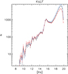 |
Fig. A.1. KLFs derived from the Ks mosaic with StarFinder, using correlation thresholds of 0.6 (blue line), 0.7 (black), and 0.9 (red). |
Appendix B: Additional results for MC simulation
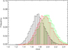 |
Fig. B.1. Best fit reduced chi2 values for the fits to the MC simulated data for mean [Fe/H] of solar (green), 1.5 solar (black), and 2.0 solar (red). |
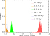 |
Fig. B.2. Histograms of the stellar mass fraction formed in given age ranges derived from fits to MC simulations of the cumulative KLF with BaSTI isochrones and assuming a mean [Fe/H] of 1.0 times solar. |
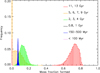 |
Fig. B.3. Histograms of the stellar mass fraction formed in given age ranges derived from fits to MC simulations of the cumulative KLF with MIST isochrones and assuming a mean [Fe/H] of 1.5 times solar. |
Appendix C: Tables of detected sources
Detected point sources in the NACO Ks and H-band large field mosaics.
Detected point sources in the deep, central NACO Ks holographic image.
Appendix D: Cumulative KLF fits with different theoretical isochrones
Best model fits to the cumulative KLF, considering stellar populations of 16 different ages and different metallicities, using PARSEC isochrones.
Best model fits to the cumulative KLF, considering stellar populations of 16 different ages and different metallicities, using MIST isochrones.
All Tables
Best model fits to the KLF, considering stellar populations of 16 different ages and different metallicities.
Best model fits to the cumulative KLF, considering stellar populations of 16 different ages and different metallicities, with and without spectroscopically confirmed young stars.
Power-law index α of a single power-law fitted to the projected surface density of stars around Sgr A* in one-magnitude wide brightness bins.
Best model fits to the cumulative KLF, considering stellar populations of 16 different ages and different metallicities, using PARSEC isochrones.
Best model fits to the cumulative KLF, considering stellar populations of 16 different ages and different metallicities, using MIST isochrones.
All Figures
|
Fig. 1. Upper left: deep image after combining all 2012 Ks exposures with the holography technique. Lower left: deep image after combining all 2012 Ks exposures with the SSA technique. The insets on the right hand side show magnifications of the areas marked by the green squares. Colour scales are logarithmic. The axes mark offsets from Sgr A* along Right Ascension and Declination in arcseconds. |
| In the text | |
|
Fig. 2. Photometric and astrometric uncertainties in the central, 9.72″ × 9.72″ field. Upper plot: 1σ uncertainty of the measured Ks magnitude of the detected stars plotted over the corresponding Ks magnitude. Lower plot: 1σ relative astrometric uncertainties. Red crosses refer to stars measured in the holographic image. Black triangles mark stars measured in the SSA image. |
| In the text | |
|
Fig. 3. KLF for the stars detected in the holographic image (red) and in the SSA image (black). |
| In the text | |
|
Fig. 4. Completeness as a function of stellar magnitude for the central field. The horizontal line indicates 50% completeness due to crowding. |
| In the text | |
|
Fig. 5. Upper panel: HKs colour magnitude diagram (CMD) for our data (large field). Colour cuts for the creation of the extinction map to exclude foreground stars, highly reddened stars, and faint stars, where the H-band data become incomplete, are indicated by dashed lines. Blue diamonds mark spectroscopically identified young, massive stars. Lower panel: extinction corrected CMD. |
| In the text | |
|
Fig. 6. KLF for the large field (black), after exclusion of foreground sources, correction for completeness due to crowding, and correction for differential extinction, assuming a mean extinction of AKs = 2.62. The blue and red lines are the KLFs of the same data, but for the region inside (blue) and outside (red) of a projected radius of 0.5 pc around Sgr A*. The red and blue lines have been scaled by an arbitrary factor to match at Ks > 14. |
| In the text | |
|
Fig. 7. Comparison between the KLF of the large field (blue, scaled by an arbitrary factor to facilitate comparison) and the KLF for the central field (black) (both LFs corrected for differential extinction and for completeness due to crowding, with foreground sources excluded). |
| In the text | |
|
Fig. 8. Minimum reduced χ2 plotted against number of single age stellar populations that are used to fit the measured KLF. |
| In the text | |
|
Fig. 9. Star formation histories for five single age events with different mean metallicities. Not all data points can be clearly seen because they bunch together at young ages. |
| In the text | |
|
Fig. 10. Top: best fit of the KLF (foreground sources excluded, corrected for differential extinction and for completeness due to crowding) with 16 single age populations for 1.5 times solar [Fe/H] (Col. 4 in Table 2). Violet: 13, 11, 9, 7 Gyr; green: 2 and 3 Gyr; blue: ≲0.5 Gyr. Bottom: same, but for the cumulative KLF (Col. 4 in Table 3). |
| In the text | |
|
Fig. 11. Histograms of the stellar mass fraction formed in given age ranges derived from fits to MC simulations of the cumulative KLF with BaSTI isochrones and assuming a mean [Fe/H] of 1.5 times solar. |
| In the text | |
|
Fig. 12. Projected stellar surface density in the deep field. Left: one-magnitude wide bins. Right: two-magnitude wide bins (the brightest bin contains all stars Ks < 15. The dashed lines show simple power-law fits. |
| In the text | |
|
Fig. 13. Relative star formation rate in the NSC as a function of time. Histograms corresponding to the SFH from the lower panel of Fig. 11 divided by the approximate length of the corresponding time intervals. |
| In the text | |
|
Fig. 14. Fraction of observed stars older than 10 Gyr as a function of magnitude at the GC, based on the MC modelling of the data with BaSTI models and mean [Fe/H] of 1.5 solar (corresponding to the SFH shown in Fig. 11). The lines correspond to cumulative probabilities of the simulations: 5% or less of the MC runs (blue dotted), 50% or less of the MC runs (black solid), 95% or less of the MC runs (red dotted). |
| In the text | |
|
Fig. A.1. KLFs derived from the Ks mosaic with StarFinder, using correlation thresholds of 0.6 (blue line), 0.7 (black), and 0.9 (red). |
| In the text | |
|
Fig. B.1. Best fit reduced chi2 values for the fits to the MC simulated data for mean [Fe/H] of solar (green), 1.5 solar (black), and 2.0 solar (red). |
| In the text | |
|
Fig. B.2. Histograms of the stellar mass fraction formed in given age ranges derived from fits to MC simulations of the cumulative KLF with BaSTI isochrones and assuming a mean [Fe/H] of 1.0 times solar. |
| In the text | |
|
Fig. B.3. Histograms of the stellar mass fraction formed in given age ranges derived from fits to MC simulations of the cumulative KLF with MIST isochrones and assuming a mean [Fe/H] of 1.5 times solar. |
| In the text | |
Current usage metrics show cumulative count of Article Views (full-text article views including HTML views, PDF and ePub downloads, according to the available data) and Abstracts Views on Vision4Press platform.
Data correspond to usage on the plateform after 2015. The current usage metrics is available 48-96 hours after online publication and is updated daily on week days.
Initial download of the metrics may take a while.