| Issue |
A&A
Volume 641, September 2020
|
|
|---|---|---|
| Article Number | A142 | |
| Number of page(s) | 17 | |
| Section | Stellar structure and evolution | |
| DOI | https://doi.org/10.1051/0004-6361/201935392 | |
| Published online | 23 September 2020 | |
Validating post-AGB candidates in the LMC and SMC using SALT spectra⋆,⋆⋆
1
Nicolaus Copernicus Astronomical Center, Rabiańska 8, 87-100 Toruń, Poland
e-mail: szczerba@ncac.torun.pl
2
Space Radio-Diagnostics Research Centre, University of Warmia and Mazury in Olsztyn, 10-719 Olsztyn, Poland
3
Main Astronomical Observatory, NASU, Zabolotnoho 27, 03680 Kyiv, Ukraine
4
Department of Physics and Astronomy, Valparaiso University, Valparaiso, IN 46383, USA
5
Space Telescope Science Institute, 3700 San Martin Drive, Baltimore, MD 21218, USA
6
Warsaw University Astronomical Observatory, Al. Ujazdowskie 4, 00-478 Warszawa, Poland
7
Laser Center, Faculty of Physics and Mathematics, University of Latvia, Raina bulvaris 19, LV-1586, Riga, Latvia
8
Nicolaus Copernicus Astronomical Center, Bartycka 18, 00-716 Warszawa, Poland
Received:
4
March
2019
Accepted:
22
June
2020
We selected a sample of post-AGB candidates in the Magellanic Clouds on the basis of their near- and mid-infrared colour characteristics. Fifteen of the most optically bright post-AGB candidates were observed with the South African Large Telescope in order to determine their stellar parameters and thus to validate or discriminate their nature as post-AGB objects in the Magellanic Clouds. The spectral types of absorption-line objects were estimated according to the MK classification, and effective temperatures were obtained by means of stellar atmosphere modelling. Emission-line objects were classified on the basis of the fluxes of the emission lines and the presence of the continuum. Out of 15 observed objects, only 4 appear to be genuine post-AGB stars (27%). In the SMC, 1 out of 4 is post-AGB, and in the LMC, 3 out 11 are post-AGB objects. Thus, we can conclude that the selected region in the colour-colour diagram, while selecting the genuine post-AGB objects, overlaps severely with other types of objects, in particular young stellar objects and planetary nebulae. Additional classification criteria are required to distinguish between post-AGB stars and other types of objects. In particular, photometry at far-IR wavelengths would greatly assist in distinguishing young stellar objects from evolved ones. On the other hand, we showed that the low-resolution optical spectra appear to be sufficient to determine whether the candidates are post-AGB objects.
Key words: stars: AGB and post-AGB / stars: abundances / stars: atmospheres / stars: emission-line, Be
The final spectra are only available at the CDS via anonymous ftp to cdsarc.u-strasbg.fr (130.79.128.5) or via http://cdsarc.u-strasbg.fr/viz-bin/cat/J/A+A/641/A142
© ESO 2020
1. Introduction
The stars with the initial mass range of about 1−8 M⊙ lose most of their mass during the asymptotic giant branch (AGB) phase (see e.g. Habing & Olofsson 2004, for review). Once the star leaves the AGB, it starts to increase its surface temperature and the mass loss gradually decreases. The star is heavily obscured by an expanding dusty envelope until the envelope disperses into the interstellar medium. Post-AGB1 stars comprise a group of objects in the transition stage between the AGB and planetary nebula (PN) phase. Most of them are quite faint or even undetectable in the optical. Their spectral energy distribution (SED) is dominated by a dusty shell, which is bright in the infrared. The SED show one or two distinguishable peaks (one corresponding to the shell and the other to the central star, if visible), depending on the orientation and characteristics of the dusty shell (e.g. Siódmiak et al. 2008). Only about 300 post-AGB stars are known in our Galaxy. This small number is due primarily to their short evolutionary timescale (Szczerba et al. 2007).
The Magellanic Clouds (MCs) provide an excellent environment to study stellar populations thanks to the known distances and negligible extinction. However, only about 70 optically bright post-AGB candidates have been suggested in the Large Magellanic Cloud (LMC; van Aarle et al. 2011) and 21 high-probability post-AGB candidates have been found in Small Magellanic Cloud (SMC; Kamath et al. 2014) using optical spectroscopy. Kamath et al. (2015) extended the analysis of van Aarle et al. (2011), and selected 35 likely post-AGBs in the LMC on the basis of determined stellar parameters.
We selected a sample of post-AGB candidates in the MCs using solely the infrared colours (for details, see Sect. 2) of known post-AGB stars from our Galaxy and the MCs. The selected region on the colour-colour diagram (CCD) is not free from other kinds of objects, namely planetary nebulae, young stellar objects (YSOs), or Seyfert galaxies. While these objects have different spectral characteristics in the optical than post-AGB stars, they could have similar photometric colours or magnitudes. However, Seyfert galaxies can be easily distinguished by means of the radial velocity shift, while PNe show highly excited emission lines requiring a hot central source.
We performed spectroscopic observations of the brightest objects in optical wavelengths. The sample was selected on the basis of the optical photometry from Zaritsky et al. (2004) for the LMC and Zaritsky et al. (2002) for the SMC. In one case, data from the NOMAD catalogue (Zacharias et al. 2004) were used. The immediate goal is to know which objects in the sample belong to the small class of post-AGB objects so that we might add to the confirmed sample and better understand their properties, while the overall goal is to determine the fraction of post-AGB stars and other types of objects (planetary nebulae, young stellar objects) that are present in the infrared-selected sample.
The paper is organised as follows. In Sect. 2 we describe our criteria used for the selection of post-AGB candidates in the MCs, and in Sect. 3 we describe briefly their South African Large Telescope (SALT) observations and present complementary photometric data. In Sect. 4 we discuss results, starting with emission-line objects and then the objects with absorption lines in their spectra. Model atmospheres are used to determine physical parameters of the latter group. Finally, we present the discussion and summary.
2. Selection of post-AGB candidates
van Aarle et al. (2011) identified some high-probability post-AGB objects in the LMC, using a combination of infrared photometry from the Spitzer Space Telescope (SST: Werner et al. 2004) and ground-based optical data. The work on selecting post-AGB candidates in the LMC was then extended by Kamath et al. (2015). A similar work to search for optically visible post-AGB candidates in the SMC was carried out by Kamath et al. (2014). Interestingly, post-red giant branch (post-RGB) stars were recognised in the SMC and LMC by Kamath et al. (2014) and Kamath et al. (2015), respectively. In addition, the authors show that SEDs indicative of discs (results of binary evolution) are dominant among post-AGB and post-RGB objects.
In all these works spectroscopic confirmation (determination of the stellar parameters from the spectral observations) was still necessary to recognise the real nature of the object. However, the large initial number of candidates required a correspondingly large number of spectra to be obtained. For example, Kamath et al. (2014) obtained spectra for 801 SMC objects to find out that 21 of them are “likely post-AGB” and 42 are post-RGB objects (about 8%), while in the case of the LMC Kamath et al. (2015) classified 35 sources as “likely post-AGB”, and 119 as post-RGB objects by analysis spectra for 2102 sources (i.e. about 7% are confirmed post-AGB and/or RGB objects).
In general, there are no good mid-IR colour-colour or colour-magnitude criteria for selecting post-AGB candidates. The AGB stars, which generally have simpler geometry of circumstellar shells than post-AGB objects, can be more easily recognised on CCDs or colour-magnitude diagrams (CMDs; see e.g. Blum et al. 2006; Sewiło et al. 2013; Matsuura et al. 2014). For example, the CMDs discussed by Blum et al. (2006) are shown for LMC objects from Jones et al. (2017) in Appendix A. While some groups of objects (like AGBs, massive stars, or planetary nebulae) are located in relatively distinct regions of the CCDs, the post-AGB objects are highly mixed with these groups (especially with YSOs and PNe).
To select post-AGB candidates in the Magellanic Clouds, we used K-[8] versus K-[24] CCD. This diagram can be used for sources with and without known distances. We verified that among different CCDs constructed from near-IR and SST photometry, this CCD is the best suited for separating evolved stars from other types of objects (Szczerba et al. 2016; Matsuura et al. 2014; Jones et al. 2017). Both O- and C-rich AGB stars are nicely separated on this diagram and there is a region where post-AGB objects are located as well, but mixed especially with young stellar objects (Szczerba et al. 2016; Jones et al. 2017). The colour indices constructed using wavelengths longer than 24 μm would serve better as a discriminator between evolved and young stars. The reason is that very often YSOs are embedded in their parental cloud and this results in a larger far-IR excess than is observed from post-AGB objects. However, IRAS (Neugebauer et al. 1984), AKARI (Murakami et al. 2007), and SST observations at longer wavelengths are not as numerous for the MCs objects as are the SST photometric data at 24 μm. For the post-AGB candidates in the LMC and SMC on this CCD, we used K photometry from 2MASS and 8 and 24 μm SST photometry from the Surveying the Agents of a Galaxy’s Evolution (SAGE) project (Meixner et al. 2006) for the LMC and SAGE-SMC (Gordon & SAGE-SMC Spitzer Legacy Team 2010).
The first step was to identify the region on this CCD which contains most of the known post-AGB objects. For this purpose we used a sample of Galactic post-AGB objects from the Torun catalogue (Szczerba et al. 2007, 2012). In Fig. 1 we present their distribution, based on synthetic photometry from their Infrared Space Observatory (ISO) spectra, as black star symbols (Galactic post-AGB in the inset on Fig. 1). The sample of post-AGB candidates in the LMC and SMC, known to us at the time of the SALT proposal preparation, from Volk et al. (2011), are plotted as cyan squares (Volk11_C-PAGB). The selection of post-AGB candidates in Volk et al. (2011) was based on the SAGE-Spec Spitzer Legacy Program (Kemper et al. 2010). Using triangles of different colours and orientations we show the positions of newly discovered (RP06-newPN) and previously known (RP06-oldPN) LMC planetary nebulae from Reid & Parker (2006), as well as those from Leisy & Dennefeld (2006) (LD06-PN). The number of sources plotted, limited by available photometry of good quality, is shown in parentheses in the inset.
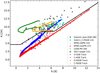 |
Fig. 1. Colour–colour diagram used for the selection of the post-AGB candidates. The main post-AGB candidate area is above the black lines. The numbers in parentheses in the inset list the total number of each class of objects plotted in this figure (see text for details). |
In addition, in Fig. 1 we overplot positions of self-consistent time-dependent hydrodynamical (HD) radiative transfer calculations for gaseous dusty circumstellar shells around C-rich and O-rich stars in the final stages of their AGB/post-AGB evolution. These calculations are based on the evolutionary track for a star with an initial mass of 3.0 M⊙, which, due to mass loss, is reduced to a typical mass for central stars of post-AGB objects of 0.605 M⊙ (Bloecker 1995) at the end of the AGB evolution. We used a single dust grain size (a = 0.05 μm) for both chemical compositions: amorphous carbon (AC) and astronomical silicates (ASil) (see Steffen et al. 1998, for details). The HD evolutionary track for AC dust is shown by red/orange dots (C-AGB Track/C-PAGB Track in the inset on Fig. 1), while for ASil dust by blue/green dots (O-AGB Track/O-PAGB Track) for the AGB/post-AGB phase, respectively. The HD models are plotted in equidistant intervals in time (100 years for AGB and 0.3 year for post-AGB), so the density of the points is a direct measure of the probability of finding various objects in different parts of the diagram. The last 200 years during AGB (the quick transition to post-AGB phase) are plotted each 20 years. The AGB phase covers 350 000 years, while the post-AGB only about 1000 years. While new models for the evolution of post-AGB stars exist (Miller Bertolami 2016), their much faster evolution results in optically thicker circumstellar envelopes for the post-AGB models, thus resulting in a smaller loops in the diagram. For the purpose of post-AGB candidates selection, the older evolutionary tracks of Bloecker (1995) seem to be sufficient and appropriate.
Taking into account the distribution of different classes of sources as well as the position of post-AGB HD tracks, we defined somewhat arbitrarily a region which should contain post-AGB objects. This region is located in the upper left portion of Fig. 1. The boundary points, which allow us to reconstruct the lines delineating the lower boundary of the post-AGB region in the (K-[8.0], K-[24]) plane are (−1.0, 4.6), (0.75, 4.6), (4.4, 8.6), (6.5, 8.6), and (14.0, 17.5). Although these boundary lines were based on post-AGB objects from the Galaxy, for the purpose of selecting post-AGB candidates in the two MCs, we assume that they lie in the same region on the colour-colour plane. We note that K-[8.0] minimum and maximum values are arbitrary, and are related to the size of the plot. The selected objects are distributed within 0 < K − [8.0] < 12 (see below).
Altogether we selected 716 and 274 post-AGB candidates in the LMC and SMC, respectively, in this way. However, this approach does not guarantee that only post-AGB objects are selected. We should expect contamination by other sources with similar SEDs in the 2–24 μm range, like oxygen-rich AGB stars, PNe, and especially YSOs (see e.g. Szczerba et al. 2016). To test our selection criteria for post-AGB candidates, we selected a small subsample of 15 post-AGB candidates (SALT-target in the inset on Fig. 1) in order to validate their nature with the SALT telescope. We selected the brightest post-AGB candidates (the faintest has 16.6 mag in V). For these candidates we expected to obtain S/N ≥ 30, which would be sufficient for spectral type classification. In addition, we observed for comparison purposes one relatively bright star with a spectral type similar to that expected for the post-AGB stars, the yellow supergiant Sk 105. The observed sources are listed in Table 1. This table contains for each source its running number (SK 105 does not have an attributed running number); SAGE designation, short name, and 2 MASS designation (and IRAS and other names if they exist); and coordinates (sources are ordered according to right ascension, RA) taken from the SAGE catalogues. Four of our post-AGB candidates come from the SMC, while 11 are from the LMC.
Designations and positions for the standard star and post-AGB candidates in the Magellanic Clouds.
3. Observations
We made our observations with the Robert Stobie Spectrograph mounted on the South African Large Telescope (SALT). Two settings were used. The red setting used the 900 l mm−1 grating and an 8 arcmin long, 1.2 arcsec wide slit. The spectrum covered the wavelength range 6160−9140 Å, with two gaps, 7130−7200 Å and 8170−8220 Å, and a resolution of R = 1500 (1 Å pix−1) at the central wavelength. The blue setting used a slit similar to that of the red setting and the 3000 l mm−1 grating. It covered the wavelength range 3280−4090 Å, with the gaps 3550−3580 Å and 3840−3850 Å, and a resolution of R = 3000 (0.25 Å pix−1) at the central wavelength. The log of observations is shown in Table 2, which contains date of observations, the object running number (see Table 1 for these numbers), short object name, setting, V magnitude, and the exposure time. Observations were repeated when the observing conditions did not meet the proposal criteria. Table 3 contains photometry and errors of the observed sources at U, B, V, J, H, K, [3.6], [4.5], [5.8], [8.0], and [24] (see the table notes for the source of the photometry).
Log of spectroscopic observations.
Photometry for the standard star and the Magellanic Clouds post-AGB candidates.
4. Results
In the observed sample one object (J004747) has a rather featureless spectrum, ten objects show emission lines, or emission and absorption lines in their spectra (see Fig. 2), while five objects show clear absorption-line spectra (including the standard star Sk 105) (see Fig. 3). We classified objects with the absorption lines according to the MK system (Jacoby et al. 1984) and performed quantitative analysis with atmospheric modelling to derive their basic physical parameters.
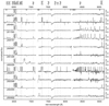 |
Fig. 2. Red spectra of the objects showing emission lines or emission and absorption lines. The spectra were normalised to continuum. A constant offset of 2.5 was applied between the adjacent spectra. Telluric lines are indicated by wheel cross symbols at the top of the plot. Vertical dashed lines give rest wavelength of the indicated emission lines. For clarity, lines representing Fe II emissions are not described. |
For emission-line spectra, we analysed these line intensities and measured radial velocities of emission lines present in the spectra in order to assign them to the relevant object class. We also inspected the 2D spectra in order to look for diffuse emission that could result from proximity of star forming regions. Our results are summarised in Table 4, which contains the object running number, short object name, classification of the object according to the literature, spectral class obtained tentatively from the comparison of the spectra with the spectra by Andrillat et al. (1995), the effective temperature determined from our atmosphere modelling, log of the surface gravity obtained from our atmosphere modelling, and remarks on the given object.
Summary of the results.
4.1. Emission-line objects
In Fig. 2 we present the red spectra of the objects clearly showing emission, and in two cases (J045907, J054055) also showing absorption lines of He I. The objects are plotted in order of increasing RA There are three SMC and eight LMC objects in the plot. Below we discuss in detail their spectra.
Object No.1: (see Table 1) J004747 is an O7 dusty star (Sheets et al. 2013). The SALT spectrum shows weak Hα emission superimposed on strong featureless continuum (top spectrum in Fig. 2). Most probably it is residual emission not well subtracted from the background. No other spectral features have been identified in the spectrum allowing for the object classification. Diffuse background emission suggests that it is located in an emission region and is likely a relatively young object.
Object No.2: J004841 shows [S III] 6312 Å and 9069 Å lines and likely the [Ar III] 7751 Å line on a detectable continuum. The object resides in a faint extended Hα emission region, and was considered a very low excitation (VLE) object by Meyssonnier & Azzopardi (1993) and classified as a young stellar object (YSO) of B0 V? spectral type by Sheets et al. (2013). In addition, Oliveira et al. (2013) classified this object as a candidate YSO.
Objects No.4: J011542 and No.5: J045747 have very similar spectra: both show very strong Hα emission, exceeding by far any other lines in the spectrum, with broad wings and no detectable [N II] 6583/6548 Å lines. Instead, they show Fe II and oxygen emission lines in the spectra. Paschen series lines in emission dominate in the red part of the spectra. These characteristics fits the criteria of the so-called Be phenomenon (Zickgraf 2000). However, these stars have strong IR excess, which is due to circumstellar dust not to free-free emission as in classical Be stars. Therefore, they are likely Herbig Ae/Be (HAeBe) stars. The diffuse background emission, which is detected in the spectra of both these objects (see Table 4) and indicates that there is a lot of matter in the vicinity of both stars, supports their classification as young objects.
J045747 has a Spitzer spectrum and Jones et al. (2017) classified it as YSO4. As we have checked, its bolometric luminosity is of the order of 45 000 solar luminosities, and there is no doubt that this is a massive Herbig Ae/Be star taking into account the above-discussed properties; we note, however, that van Aarle et al. 2011 retains J045747 in the catalogue of post-AGB candidates. On the other hand, Kamath et al. (2014) classified J011542 as a hot post-AGB/RGB candidate. We estimated that the bolometric luminosity is about 18 000 solar luminosities, and in principle it could be a massive post-AGB object. However, the similarity of features observed in the optical spectra of both objects suggests that it is also a Herbig Ae/Be object.
Object No.6: J045907 and No.14: J054055 both show strong H α together with [N II] 6584/6548 Å emission, and 6678 Å and 7065 Å He I absorption lines. In addition, emission lines of Si II 6347 Å and 6371 Å, [S III] 6312 Å and 9069 Å, [S II] 6716/6731 Å, and [O II] 7319/7330 Å are seen in the spectra. J045907 was classified as a O9ep/B1-2ep star by van Aarle et al. (2011) and was not considered a post-AGB star, due to its excessively high luminosity. Our spectrum suggests an O type (possibly O9e:), but it relies only on two He I lines (6678 Å and 7065 Å) seen in absorption. Similarly, J054055 has been classified as O-B type by van Aarle et al. (2011), and was not considered a post-AGB star, due to its observed luminosity exceeding the upper limit expected for a post-AGB star. Our spectrum suggests O type (possibly O9), but again it relies on only two He I absorption lines at 6678 Å and 7065 Å.
Object No.8: J051228 shows only Hα, [N II] 6584/6548 Å, He I 7065 Å, and O I 8446 Å lines superimposed on relatively strong continuum in its spectrum. A planetary nebula central star would have a much weaker continuum. van Aarle et al. (2011) did not assign any spectral type for this object, but list it as a post-AGB candidate. However, a weak diffuse emission is detected in the vicinity of the object, which suggests its young age. For this reason the object appears to be a YSO or H II region rather than a post-AGB star.
Object No.10: J052229 shows Hα, [N II] 6584/6548 Å, [S II] 6716/6731 Å, and other emission lines redshifted by ∼ 10 000 km s−1 with respect to the LMC (Fig. 2). We classify it as a background galaxy, in agreement with van Aarle et al. (2011).
Object No.12: J052915 is listed as a post-AGB candidate by van Aarle et al. (2011), but it is a known PN (Reid & Parker 2010). Our observation supports this classification. The object shows strong [N II] 6584/6548 Å, [O I] 6300/6363 Å, [S II] 6723/6737 Å, [O II] 7319/7330 Å, [S III] 9096/6312 Å, and [Ar III] 7751 Å lines in addition to the helium and hydrogen lines.
Objects No.13: J053348 and No.15: J055825 show very similar spectra (Fig. 2). Alcock et al. (1996) classified J053348 as a hot R CrB star with a Teff of about 20 000 K. J055825 has been classified as an He-burning AGB star (Vijh et al. 2009). Absorption lines or bands and emission lines are observed in the blue part of the spectrum of J055825 (Fig. 4). van Aarle et al. (2011) classified both objects as Wolf–Rayet carbon stars and discard them from the post-AGB sample. They noted, however, the resemblance of the spectra of both stars with that of Galactic R CrB star V 348 Sagittarius.
4.2. Absorption-line objects
In Fig. 3 we present the red spectra of the five objects with absorption lines in their spectra. First the spectrum of our standard star, Sk 105, is plotted, and then objects No. 11, 9, 7, and 3 (the only object from the SMC). We put them in order of decreasing RA to facilitate further discussion. We present our MK classification of the spectra and by comparing the synthesised colours for a given spectral class with observed values we derive total (circumstellar plus interstellar) extinction. Then we present quantitative analysis with the model atmosphere and spectra synthesis technique to derive basic physical parameters of the objects.
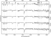 |
Fig. 3. Spectra of the absorption line or featureless objects in the red setting. The spectra were normalised to continuum. A constant offset of 1.2 was applied between the adjacent spectra. Vertical dashed lines indicate the rest wavelengths of the indicated absorption lines. |
4.2.1. MK classification
We performed the MK classification according to Gray & Corbally (2009) and standards observed by Andrillat et al. (1995). Our MK classifications relies mainly on the strength of the Ca II triplet 8498 Å, 8542 Å, and 8662 Å, blended with P16, P15, and P13 Paschen lines, relative to other lines from the Paschen sequence, which is sensitive to stellar temperature (Gray & Corbally 2009). In supergiants the Paschen lines are narrower with respect to other luminosity classes. However, it should be noted that the standards observed by Andrillat et al. (1995) are mainly (or exclusively) population I stars with higher metallicities than our targets, thus more relevant for comparison with Galactic objects. The decreased metallicity in MC objects results in reduced strength of the Ca II lines. Thus, the spectral types and stellar temperatures derived from MK classification based on the relative strength of the Ca II lines would be systematically higher. This poses the main problem and main source of uncertainties in our classification. The spectral resolution of our observations in the red setting and observations by Andrillat et al. (1995) is quite similar (about 1 Å) and should not introduce additional uncertainties.
All five objects show hydrogen Paschen series in absorption. The lines are relatively narrow and deep, which results in lines from upper levels, including those above P17, to be visible. This indicates a supergiant luminosity class. The lines identified in the spectra are listed in Table 4. The detailed discussion of the spectral type classification of each is given below.
Sk 105 is a yellow supergiant of MK spectral type F0 I (Neugent et al. 2010). Our spectrum allowed us to constrain the spectral type between A7 and F2, and luminosity class Ib. The photometric B–V colour index (see Table 3) match this spectral type quite closely, assuming negligible circumstellar or interstellar extinction, and the corresponding effective temperature for the assigned F0Ib spectral type is 7460 K (Cox 2000).
Object No.11: J052520 is a C-rich post-AGB star with a strong 21 μm dust feature (Volk et al. 2011; Matsuura et al. 2014); Sloan:2014uq. This object varies with a periodicity between 34 and 45 days, but does not have a stable dominant period (Hrivnak et al. 2015). From their low-resolution spectra, van Aarle et al. (2011) determined the spectral type of this object as A1Ia (about 9700 K; Cox 2000), and estimated its effective temperature from the SED to be 9250 ± 250 K. However, Matsuura et al. (2014) derived a spectral type of F2-F5 I, with reference to the spectral atlas of Jacoby et al. (1984), based on strong Ca II H and K, weak G band, sharp weak H line absorption, and strong O I 7774 Å seen in their spectrum.
J052520 was observed in the red and blue settings with SALT (see blue spectrum in top panel of Fig. 4). We classify this star as an A2Ib type (about 9000 K; Cox 2000). Clearly, the Ca II triplet is less pronounced than in Sk 105, indicating earlier spectral type. Strong Ca II H and K lines present in the blue part of the spectrum indicate, on the other hand, A0 type or later. The spectrum shows strong Sr II 4077 Å line, confirming luminosity class I. J052520 clearly shows an s-process Ba element line at 6496 Å (see further discussion). The observed colour B − V = 1.25 (Zaritsky et al. 2004), with a spectral type of A2I ((B − V)0 = 0.03; Cox 2000) indicates a total (circumstellar plus interstellar) reddening EB − V of about 1.2.
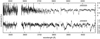 |
Fig. 4. Spectra of objects in the blue setting. The spectra are normalised to continuum. |
Object No.9: J052043 is another C-rich post-AGB star with a strong 21 μm dust feature (Volk et al. 2011); Matsuura:2014ve; Sloan:2014uq. It has a complicated variability pattern with dominant period of about 74 days (Hrivnak et al. 2015). This object is classified as a F5Ib(e) type (about 6400 K; Cox 2000) by van Aarle et al. (2011), or F8I(e) (about 5750 K; Cox 2000) by Hrivnak et al. (2015). J052043 clearly shows an s-process Ba element line at 6496 Å (see further discussion). We assign F5I spectral type (about 6370 K; Cox 2000) for this object based on the strength of Ca II triplet compared to Pa series. The observed colour B − V = 1.44 (Zaritsky et al. 2004), with a spectral type of F5I ( (B − V)0 = 0.32; Cox 2000) indicates a total reddening EB − V of about 1.1.
Object No.7: J051110 is also a C-rich post-AGB star with 21 μm dust feature (Volk et al. 2011; Matsuura et al. 2014; Sloan et al. 2014)). This object shows clear evidence of variability with two significant periods of about 112 and 96 days (Hrivnak et al. 2015). van Aarle et al. (2011) determined the spectral type of this object as F3II(e) type (about 6800 K for luminosity class I; Cox 2000), or slightly more for luminosity class II, which agrees with Teff of 7000 ± 250 K obtained from their SED modelling. We classify it as F0Ib type (about 7460 K; Cox 2000), but with large uncertainty. J051110 also shows an s-process Ba element line at 6496 Å (see further discussion). The observed colour B − V of about 1.8 (Zaritsky et al. 2004), with a spectral type of FOIb ((B − V)0 = 0.17 for luminosity class I object; Cox 2000) indicates a total reddening EB − V of about 1.6. Clearly, the object is heavily reddened.
Object No. 3: J010546 is the only SMC object in our sample with stellar absorption lines in its spectrum. It shows relatively weak Hα emission with broad wings superimposed on continuum, and some weak absorption lines. The Ca triplet does not appear to be superimposed on a Paschen series. The O I line at 7774 Å is visible, as are the Si II 6347, 6371 Å lines. The best fit to the standards was achieved for B8 Ia/b type (temperature of about 11 100 K; Cox 2000). The observed colour indicates the total reddening EB − V of about 0.4 for this object. This source also shows the 21 μm feature (Volk et al. 2011; Sloan et al. 2014), so it is a C-rich post-AGB star. Kamath et al. (2014) list it as a hot post-AGB/RGB candidate.
4.2.2. Synthetic spectra: analysis procedure
A grid of model atmospheres of supergiants2 was computed using the SAM12 program (Pavlenko 2003). SAM12 is a modification of the ATLAS12 code of Kurucz (1993). When computing cooler model atmospheres (Teff ≤ 9000 K), we modelled the convective energy transport using mixing-length theory with the ratio of mixing length to scale height l/h = 1.6. The line opacity was used in the framework of opacity sampling technique (Sneden et al. 1976) with the VALD2 atomic list (Kupka et al. 1999).
We computed model atmospheres of effective temperatures Teff = 5250−8000 K with steps of 250 K and Teff = 9000 K; gravities log g = 0, 0.5, 1 for the cooler models and log g = 1.5−2.5 for the hotter models (step of 0.5 in log g ); and metallicities [Fe/H] = 0, −0.2, −0.5, −1, −1.5, −2, −2.5. Since these objects are all C-rich, we then computed model atmosphere grids for a set of [C/O] = +0.2, +0.4. We found that the dependence of our results on [C/O] is marginal; nevertheless, we carried out our analysis for different values of [C/O]. For analysis of the hottest star in our sample we computed an additional set of hot model atmospheres of Teff from 10 000 to 20 000 K, with step of 1000 K and log g = 2.0−3.5.
The technique of synthetic spectra was used to carry out our analysis of the observed spectra computed with the WITA6 program (Pavlenko 1997) within the classical framework. A microturbulent velocity of Vt = 3.5 km s−1 was adopted. Our synthetic spectra were computed with wavelength steps of 0.025 Å, which provided detailed profiles of all the lines.
In the most general case the quality of the fits to the observed spectra depends on many adopted parameters: effective temperature, gravity, microturbulent velocity, and the abundances of elements. In this paper we solve a restricted case using fits to the selected narrow spectral region 8450−8800 Å. Unfortunately, we do not have good enough data to provide the detailed numerical analysis of the abundance of all elements. Therefore, we used the parameter of metallicity for most of the elements, except for carbon and s-elements. Some s-process elements are so overabundant that their lines are seen in the spectra of the absorption-line objects. This allowed us to estimate their abundances (see Sect. 4.2.4).
The observed spectra are broadened by macroturbulence and by instrumental broadening; both are implemented in the modelling by smoothing the computed spectra with a correspondent Gaussian, which is a reasonable approach for fitting stellar spectra. The appropriate values of full width at half maximum were determined from every spectrum during the procedure of finding the best fit to the observed spectrum.
Using the standard χ2 procedure to determine the best fit of synthetic spectra (Ssynt) from our grid to the observed spectrum (Sobs), we find the minimum of the 3D functional

where fh is the flux normalisation coefficient, fs is the wavelength shift between the theoretical and observed spectra, and fg a parameter of convolution describing the broadening by macroturbulent motions and instrumental broadening. The observed spectra had been normalised to the continuum/pseudo-continuum prior modelling.
4.2.3. Fits to the observed spectra
The parameters of the stellar atmospheres were obtained from the fits to the H I Paschen lines and the Ca II triplet at 8498 Å, 8542 Å, and 8662 Å lines. All three Ca lines were blended with the H I Paschen lines at the resolution of our red spectra. This is demonstrated in Fig. 5, which shows an example of a synthetic spectrum without hydrogen (red line) where the Ca II triplet lines are clearly seen, and a spectrum of pure hydrogen (green line) where the subsequent lines of the H Paschen series are identified. It is worth noting that for a given metallicity, Ca lines become weaker on the hot edge of our temperature range, while the strength of H lines increases at the same time. Thus, this spectral region provides a good opportunity for the self-consistent determination of Teff and [Fe/H]. For simplicity, we made the reasonable assumption that the abundance of Ca follows the trend of [Fe/H].
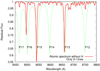 |
Fig. 5. Synthetic spectrum computed from a model atmosphere without hydrogen (red line), and synthetic spectrum of pure hydrogen atmosphere (green line). The Ca II triplet 8498 Å, 8542 Å, and 8662 Å lines are clearly seen in the red spectrum. The subsequent transitions of the hydrogen Paschen series seen in the green spectrum are indicated in the plot. |
All observed spectra were affected by fringing, which possessed an amplitude of about 10% on the red side. This restricted the accuracy of our fit. Nevertheless, using the procedure of fitting the observed spectra in the spectral region of the Ca II and Paschen lines, we were able to determine Teff and log g. In our case, the formal error in the measured quantities should be equivalent to the lowest step in the grid, namely 250 K in Teff and 0.5 in log g.
Due to the broad profiles and blending effects of the Paschen H I photospheric lines, it is very difficult to perform proper normalisation of the spectra with respect to the local continuum level for the Paschen series lines. Thus, after preliminary modelling we normalised the spectra to the continuum for a second time. Then the modelling was performed again to get more accurate stellar parameters.
We began by testing our modelling procedure by fitting the spectrum of the supergiant Sk 105, observed by us as a template star. Sk 105 is the brightest star in our sample and was observed with the best S/N. Results of the fit to the Sk 105 spectrum are shown in Fig 6. The best fit to the observed spectrum, determined primarily by fitting the H Paschen lines and Ca II subordinate triplet at 8498, 8542, and 8662 Å, provides our estimation of its effective temperature, gravity, metallicity, and [C/O]: 6500/0.5/-0.5/0.0. Our estimation of Teff is quite similar to the value of Teff = 6800 K derived by Neugent et al. (2010). The presence of Paschen lines of H I and lines of the Ca II triplet of the observed strength qualitatively agree with our Teff estimation.
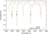 |
Fig. 6. Best fit of the synthetic spectrum computed for a model atmosphere with effective temperature, gravity, metallicity, and [C/O]: 6500/0.5/−0.5/0.0 (green line) to the observed spectrum of Sk 105 (red line). Arrows indicate the Ca II lines, which are blended with H I Paschen lines. |
Following the reasonably good fit to the spectrum of Sk 105, we applied our procedure to the four objects with absorption lines in their SALT spectra. Our best fits, together with the obtained model atmosphere parameters, are shown in Fig. 7 for object No. 11: J052520, in Fig. 9 for object No. 9: J052043, in Fig. 10 for object No. 7: J051110, and in Fig. 11 for object No. 3: J010546. The obtained model atmosphere parameters confirm the post-AGB nature of each object, and they are the first such values determined for J051110 and J010546. These model atmosphere values are listed in Table 5.
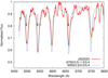 |
Fig. 7. Best fit of the synthetic spectrum computed for a model atmosphere of 6750/0.5/−1.5/0.4 (green line) to the observed spectrum (red line) of object No. 11: J052520. The blue line shows the best solution for the theoretical spectrum computed for model atmospheres with Teff = 9000. |
Parameters of the model atmospheres.
For J052520 the fit to the observed spectrum is fairly good (see Fig. 7) and the correctness of the parameters is supported by the good agreement of the fit to the blue part of the spectrum (see Fig. 8). The blue part of the spectrum shows strong resonance lines of Ca II at λλ 3934 and 3968 Å, which can be used as an independent check of the obtained best stellar parameters from the fits to lines in the near-IR spectrum. In Fig. 8 we compare observed blue part of the spectrum (red line) with the theoretical spectrum (green line) obtained for the best fitting parameters (see Table 5). As can be seen, the theoretical spectrum reproduces fairly well the observed Ca II lines, and the H Paschen lines, thus providing evidence that our method gives consistent results and that the obtained stellar parameters are correct.
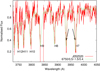 |
Fig. 8. Fit to the blue part of spectrum (red line) of object No. 11: J052520 with stellar model parameters derived from the best fit to the red spectrum of this object. The Ca II resonance lines are indicated by arrows. |
Kamath et al. (2015) has also derived stellar parameters from model atmosphere fitting to their low-resolution spectrum of this object. While their effective temperature is the same as in our model (6750 K), the metallicity and especially the gravity differ. They obtained log g = 2.5, causing them to classify the star as a young object. Since the post-AGB nature of this object is well established (presence of 21 μm feature), they argue that a large uncertainty in their log g value arises from the difficulty in fitting the Ca triplet region in spectra of this temperature and the rather noisy spectrum in the region of the Balmer lines 3750−3950 Å.
The obtained Teff of 6750 K is very different to that inferred from the MK classification of about 9000 K (see Sect. 4.2.1). In Fig. 7 we also show the best fit obtained with 9000 K. Clearly this temperature value results in hydrogen lines that are too strong. Taking into account all the above arguments we can conclude that the MK classification gives the wrong spectral type. Modelling yields the lowest metallicity for J052520 of all observed absorption-line objects, and this may be the reason for the large difference between MK classification and the model.
In the case of J052043, the fit to the spectrum is good except for the Paschen line at 8600 Å (see Fig. 9). Our spectral classification of F5I (about 6370 K) is consistent with the derived temperature of 6250 K. van Aarle et al. (2013) derived a lower temperature (5750 K) and lower metallicity ([Fe/H] = −1.0) from the analysis of their UVES spectra. In Fig. 9 we show the synthetic spectrum computed for parameters obtained by van Aarle et al. (2013). As can be seen, the hydrogen lines are too weak for Teff = 5750 K, and the Ca lines are shallower for a metallicity [Fe/H] = −1.0, as expected. One explanation for this difference could be variability of the source. J052043 has a dominant period of about 74 days (Hrivnak et al. 2015). Hrivnak et al. (2010) found that PPNe show colour changes corresponding to temperature changes of 300−700 K.
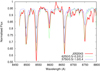 |
Fig. 9. Best fit of the synthetic spectrum computed for a model atmosphere of 6250/0.5/−0.2/0.2 (green line) to the observed spectrum (red line) of object No. 9: J052043. The blue line shows the fit to the observed spectrum with parameters 5750/0.5/−1.0 found by van Aarle et al. (2013). |
The fit for J051110 is reasonably good (see Fig. 10), but it does not fit the Ca 8500 Å line or the Paschen line at 8600 Å. The fit gives a temperature of 6750 K. This disagrees quite a bit with the temperature estimation of 7460 K based on our MK classification as F0I. However, as we mention in Sect. 4.2.1, this determination was made with a large uncertainty. On the other hand, the difference can be accounted for by stellar pulsations and related variability in temperature. We note that the value of Teff determined by our model agrees within the error with the temperature determination from MK classification or SED modelling by van Aarle et al. (2011).
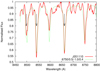 |
Fig. 10. Best fit of the synthetic spectrum computed for a model atmosphere of 6750/0.5/−1.0/0.4 (green line) to the observed spectrum of object No.7: J051110. |
J010546 is the hottest star among our absorption-line objects. It shows relatively weak lines of hydrogen and ionised calcium, which both indicate a rather high effective temperature. Our fit indicates that the temperature of J010546 is in the range 10 000−15 000 K (see Fig. 11), which agrees with the MK classification of B8I (11 100 K). In general, the results of the best fit depend on the adopted continuum level in the selected spectral range. For this source the structure of the spectrum is quite complicated, and the continuum level is poorly determined. Therefore, we performed fits for two adopted continuum levels in the observed spectrum. Results for the continuum at 1.0 and 1.03 are shown in Fig. 11 as the green and blue line, respectively. Both models reproduce the P12–P15 lines of hydrogen and the Ca II lines fairly well. However, the formal goodness S = 0.750 ± 0.003 is slightly better for the fit with Teff = 15 000 K than S = 0.890 ± 0.004 for Teff of 10 000 K.
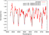 |
Fig. 11. Best fit of the synthetic spectra computed for model atmospheres of 15 000/2.5/0.0/0.4 (green line) and 10 000/3.0/0.0/0.2 (blue line) to the observed spectrum (red line) of object No. 3 J010546, assuming different continuum levels at 1.0 and 1.03, respectively. |
4.2.4. s-elements abundance.
As we already noted, the resolution of our spectra is not high enough to carry out accurate determination of abundances. However, we see evidence of a significant contribution of s-element lines in the spectra of our cooler absorption-line stars. As an example, in Fig. 12, we compare the spectrum of J051110, which is shown by a red line, with the spectrum of our standard star Sk 105 (green line) in the range from 6200 to 6850 Å. The positions of some transitions of s-process elements (Ba, Ce, La, Sm, Y, and Zr) are shown by vertical arrows. As can be seen, the spectrum of J051110 clearly shows absorption lines of s-process elements.
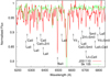 |
Fig. 12. Comparison between the spectra of J051110 (red line) and the standard star Sk 105 (green line). Positions of some s-process element transitions are identified on the plot. |
To get reliable fits to the observed spectra of our stars in the wavelength range where s-process elements are clearly seen, we increased the abundance of s-process elements during computations of the model atmospheres (see Table 6). Computations were carried out for the model atmospheres with parameters found from the fits to hydrogen Paschen and Ca II lines (Table 5). However, while fitting the atomic lines of intermediate strength in the observed spectra, we found that a microturbulent velocity Vt = 4.5 km s−1 better describes the observations of s-element absorption lines. Our numerical experiments show that the resulting changes to the model atmospheres is marginal in the case of changing Vt from 3.5 to 4.5 km s−1.
Abundances of s-elements in the atmospheres of three post-AGB stars.
The results of our fitting are shown in Fig. 13. The accuracy of the abundance determination is not high (±0.5 dex), mainly due to the low resolution of our spectra. In the case of J052520, we obtained similar results from the blue and red spectral ranges. However, the red spectral range provides less confident results. In the case of J052043, while fitting the model with the s-process elements enhanced, we reduced the abundances of Ti and Fe by −0.5 dex to get a better fit in the spectrum at 6200–6500 Å.
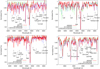 |
Fig. 13. Best fit of synthetic spectra with enhanced abundances of s-elements to the observed spectra of J051110 (top left), J052043 (top right), J052520 (bottom left), and blue spectrum of J052520 (bottom right). The fit with s-process elements enhanced to the spectrum of J052043 required a reduction in abundances of Ti and Fe of −0.5 dex. |
Finally, we note that in the spectrum of J051110, we detected a strong absorption feature near 6708 Å. Reyniers et al. (2002), in a study of post-AGB stars, identified the feature at 6708 Å as a Ce II line λ 6708.099 Å. However, to get the right fit to wavelength and strength of this feature in J051110 the contribution from Li I 6707.8 Å line seems to be necessary. In this spectral region, Ce II has three transitions at 6704.5 Å, 6706.1 Å, and 6708.1 (see e.g. Reyniers et al. 2002), which in our resolution are blended into a single line, and a strong line at 6775 Å (see red line in Fig. 14).
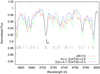 |
Fig. 14. Observed spectrum of J05110 (red line) and two fits with enhancement of Ce and no Li (green line), and with both elements enhanced (blue line). See text for more details. The vertical lines show the positions of the Ce II lines. |
In order to fit the observed intensity of the 6708 Å absorption and position of the 6775 Å line, we had to enhance the Ce abundance to [Ce/Fe] = +2.9 and to shift the theoretical spectrum by about 45 km s−1 (about 1 Å) to the right. We note that the resolution of our spectra is about 1500 and the position of each line is known with an accuracy of about 2 Å. However, this shift in wavelengths, while giving right position of the Ce II 6775 Å line, does not seem to reproduce the position of the 6708 Å blend. In addition, the assumed enhancement of Ce results in absorption that is too strong at 6775 Å (see green line in Fig. 14). One of the obvious explanations for this discrepancy is that the lithium Li I 6707.8 Å line contributes to the observed blend at 6708 Å. This fit, with the large enhancement of [Li] = +4.1 and slightly reduced overabundance of Ce ([Ce/Fe] = +2.5), is shown in Fig. 14 (blue line). The match in position and strength for both features at 6708 and 6775 Å is much better now. However, the limited resolution of our spectrum does not allow us to perform a more detailed analysis. Spectra of much higher resolutions are necessary to confirm the presence of lithium in the atmosphere of J05110. Interestingly, the other stars in our sample do not show the 6708 Å feature.
5. Discussion and conclusions
We observed fifteen optically bright post-AGB candidates and one spectroscopic standard in the MCs using the SALT telescope. The candidates were selected on the basis of the infrared colour-colour diagram [K]-[24] versus [K]-[8], residing in the region where most of the known post-AGBs and PNe, as well as our HD evolutionary tracks, are located. The spectra were obtained mainly in the red region (6160−9140 Å) and have relatively low resolution R ∼ 1500. Ten stars show emission lines or combined emission and absorption lines in their spectra, one object has an essentially featureless spectrum, and four stars have absorption-line spectra and are likely post-AGB stars. We examined the long-slit spectra for diffuse background Hα emission; it is found in most of the emission-line objects, but in none of the likely post-AGB stars. The summary of the obtained results is presented in Table 4.
Among the emission-line objects, we classify three as young stellar objects (objects No. 1, 2, and 8 according to the numbers from Table 1), two as possible Herbig Ae/Be stars (No. 4 and 5), two as massive stars probably post-main sequence (No. 6 and 14), one as a galaxy (No. 10), one as a planetary nebula (No. 12), and two as R CrB stars (No. 13 and 15, the latter classified as such for the first time).
For the four absorption-line objects (No. 3, 7, 9, and 11), we performed MK classification of the spectra and found them to range from B8 to F5 supergiants. We then fitted model atmospheres to the spectra to derive their physical parameters. The obtained model parameters confirm the post-AGB nature of the objects, and physical parameters were obtained for the first time for objects No. 3 and 7. For three of them (No. 7, 9, and 11), we calculated the approximate abundances of the s-process elements, and for object No. 11 we argued that lithium contributes to the absorption structure observed at about 6708 Å. All absorption-line objects are C-rich as they possess the characteristic 21 μm feature. However, the C/O ratio is poorly known in the atmospheres of our stars due to the lack of the appropriate absorption lines in their spectra.
Among the 15 objects from our sample, we identified 7 evolved objects (four genuine post-AGB stars, two R CrB stars, and one PN), 7 young objects (three YSOs, two massive stars, and two Herbig Ae/Be stars), and one galaxy. Thus, we can conclude that the selected region on [K]-[24] versus [K]-[8] colour-colour diagram is able to discriminate evolved objects at a success rate of about 50% (about 25% for genuine post-AGB objects). The remaining objects are YSOs or massive post-main sequence stars taking into account their circumstellar dust emission. These statistics are valid only for the brightest objects, which were selected in order to obtain optical spectroscopy with SALT at a reasonable S/N. We normally expect massive stars to be relatively rare in a general sample because they are relatively short-lived. However, by selecting the brightest objects our sample was biased toward the inclusion of massive evolved stars.
It is possible to use an independent test to check the usefulness of the area that we denoted as “post-AGB candidates area”. Recently, Jones et al. (2017) classified about 1000 Spitzer spectra for about 800 sources in the Large Magellanic Cloud. These sources cover most star evolutionary stages. Those with good photometry at K, [8], and [24] bands are plotted in Fig. 15. We counted together objects of different chemistry (C- and O-rich) for AGB and post-AGB stars, and different classes of YSOs. The numbers in parentheses in the inset indicate the total number of sources in each class plotted in the figure. In the post-AGB candidate area (above the black line) there are altogether 172 objects: 84 YSOs; 26 massive stars; 14 others; 5 AGB stars; 23 PNe; 19 genuine post-AGB stars; and 1 RCrB star. As can be seen, young objects compose more than 60% of the total number of sources, while evolved stars less than 30% of them. About 66% (19/29) of the genuine post-AGB stars are located in the selected region, but they compose only about 11% of the total number of sources above the black solid line in Fig. 15.
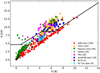 |
Fig. 15. Colour-colour diagram used for selection of the post-AGB candidates (same as in Fig. 1). The main post-AGB candidate area is above the black lines. The grouped class of objects (see text for details) from Jones et al. (2017) are plotted with different symbols. The numbers in parentheses show the total number of each class of object plotted in this figure. |
Thus the region we delineated of the [K]-[24] versus [K]-[8] colour-colour diagram as a “post-AGB candidate area” seems to select most of them, but it is populated by far more YSOs and other types of emission-line objects than it is by post-AGB stars. Photometry at longer wavelength bands would allow us to better discriminate on the basis of colour, as it was in the case with the IRAS filters (see e.g. van der Veen & Habing 1988). Until that is available, it appears that it is possible to use low-resolution spectra to eliminate the strong emission-line objects from consideration as post-AGB stars (but perhaps losing some PN). In addition, post-AGB objects of F–G spectral types are known to pulsate with periods from about 30 to about 150 days (see e.g. Hrivnak et al. 2010, 2015), so studies of light variability of the selected candidates may be helpful in identifying post-AGB objects.
The model atmospheres are available from ftp.mao.kiev.ua/pub/y/2017/postAGB/.
Acknowledgments
The spectroscopic observations reported in this paper were obtained with the Southern African Large Telescope (SALT). Polish participation in SALT is funded by grant No. MNiSW DIR/WK/2016/07. Our studies are partially supported by FP7 Project No:. 269193 “Evolved stars: clues to the chemical evolution of galaxies”. This work was co-funded under the Marie Curie Actions of the European Commission (FP7-COFUND). RSz and NS acknowledge support from the NCN grant 2016/21/B/ST9/01626 and 2014/15/B/ST9/02111. MH thanks the Ministry of Science and Higher Education (MSHE) of the Republic of Poland for granting funds for the Polish contribution to the International LOFAR Telescope (MSHE decision no. DIR/WK/2016/2017/05-1) and for maintenance of the LOFAR PL-612 Baldy (MSHE decision no. 59/E-383/SPUB/SP/2019.1). BJH was supported by NSF AST 1413660. This research has made use of the SIMBAD database, operated at CDS, Strasbourg, France. We thank the anonymous Referee for his/her thorough review and highly appreciate the comments and suggestions, which significantly contributed to improving the quality of the publication.
References
- Alcock, C., Allsman, R. A., Alves, D. R., et al. 1996, ApJ, 470, 583 [NASA ADS] [CrossRef] [Google Scholar]
- Andrillat, Y., Jaschek, C., & Jaschek, M. 1995, A&AS, 112, 475 [NASA ADS] [Google Scholar]
- Bloecker, T. 1995, A&A, 299, 755 [NASA ADS] [Google Scholar]
- Blum, R. D., Mould, J. R., Olsen, K. A., et al. 2006, AJ, 132, 2034 [NASA ADS] [CrossRef] [Google Scholar]
- Bolatto, A. D., Simon, J. D., Stanimirović, S., et al. 2007, ApJ, 655, 212 [NASA ADS] [CrossRef] [Google Scholar]
- Cox, A. 2000, Allen’s Astrophysical Quantities, 4th edn. (New York: Springer-Verlag) [Google Scholar]
- Gordon, K. D., & SAGE-SMC Spitzer Legacy Team 2010, Amer. Astron. Soc. Meet. Abstr. #215, BAAS, 42, 489 [Google Scholar]
- Gray, R. O., & Corbally, J. C. 2009, Stellar Spectral Classification (Princeton University Press) [Google Scholar]
- Gruendl, R. A., & Chu, Y.-H. 2009, ApJS, 184, 172 [Google Scholar]
- Habing, H. J., & Olofsson, H. 2004, Asymptotic Giant Branch Stars (Springer) [CrossRef] [Google Scholar]
- Hrivnak, B. J., Lu, W., Maupin, R. E., & Spitzbart, B. D. 2010, ApJ, 709, 1042 [NASA ADS] [CrossRef] [Google Scholar]
- Hrivnak, B. J., Lu, W., Volk, K., et al. 2015, ApJ, 805, 78 [NASA ADS] [CrossRef] [Google Scholar]
- Jacoby, G. H., Hunter, D. A., & Christian, C. A. 1984, ApJS, 56, 257 [NASA ADS] [CrossRef] [Google Scholar]
- Jones, O. C., Woods, P. M., Kemper, F., et al. 2017, MNRAS, 470, 3250 [NASA ADS] [CrossRef] [Google Scholar]
- Kamath, D., Wood, P. R., & Van Winckel, H. 2014, MNRAS, 439, 2211 [NASA ADS] [CrossRef] [Google Scholar]
- Kamath, D., Wood, P. R., & Van Winckel, H. 2015, MNRAS, 454, 1468 [NASA ADS] [CrossRef] [Google Scholar]
- Kemper, F., Woods, P. M., Antoniou, V., et al. 2010, PASP, 122, 683 [NASA ADS] [CrossRef] [Google Scholar]
- Kupka, F., Piskunov, N., Ryabchikova, T. A., Stempels, H. C., & Weiss, W. W. 1999, A&AS, 138, 119 [NASA ADS] [CrossRef] [EDP Sciences] [MathSciNet] [PubMed] [Google Scholar]
- Kurucz, R. 1993, ATLAS9 Stellar Atmosphere Programs and 2 km/s grid. KuruczCD-ROM No. 13 (Cambridge, Mass.: Smithsonian Astrophysical Observatory), 13 [Google Scholar]
- Leisy, P., & Dennefeld, M. 2006, A&A, 456, 451 [NASA ADS] [CrossRef] [EDP Sciences] [Google Scholar]
- Matsuura, M., Bernard-Salas, J., Lloyd Evans, T., et al. 2014, MNRAS, 439, 1472 [NASA ADS] [CrossRef] [Google Scholar]
- Meixner, M., Gordon, K. D., Indebetouw, R., et al. 2006, AJ, 132, 2268 [NASA ADS] [CrossRef] [Google Scholar]
- Meyssonnier, N., & Azzopardi, M. 1993, A&AS, 102, 451 [NASA ADS] [Google Scholar]
- Miller Bertolami, M. M. 2016, A&A, 588, A25 [NASA ADS] [CrossRef] [EDP Sciences] [Google Scholar]
- Murakami, H., Baba, H., Barthel, P., et al. 2007, PASJ, 59, S369 [NASA ADS] [CrossRef] [MathSciNet] [Google Scholar]
- Neugebauer, G., Habing, H. J., van Duinen, R., et al. 1984, ApJ, 278, L1 [Google Scholar]
- Neugent, K. F., Massey, P., Skiff, B., et al. 2010, ApJ, 719, 1784 [NASA ADS] [CrossRef] [Google Scholar]
- Oliveira, J. M., van Loon, J. T., Sloan, G. C., et al. 2013, MNRAS, 428, 3001 [NASA ADS] [CrossRef] [Google Scholar]
- Pavlenko, Y. V. 1997, Ap&SS, 253, 43 [NASA ADS] [CrossRef] [Google Scholar]
- Pavlenko, Y. V. 2003, Astron. Rep., 47, 59 [NASA ADS] [CrossRef] [Google Scholar]
- Reid, W. A., & Parker, Q. A. 2006, MNRAS, 373, 521 [NASA ADS] [CrossRef] [Google Scholar]
- Reid, W. A., & Parker, Q. A. 2010, MNRAS, 405, 1349 [NASA ADS] [Google Scholar]
- Reyniers, M., Van Winckel, H., Biémont, E., & Quinet, P. 2002, A&A, 395, L35 [NASA ADS] [CrossRef] [EDP Sciences] [Google Scholar]
- Sanduleak, N., MacConnell, D. J., & Philip, A. G. D. 1978, PASP, 90, 621 [NASA ADS] [CrossRef] [Google Scholar]
- Sewiło, M., Carlson, L. R., Seale, J. P., et al. 2013, ApJ, 778, 15 [NASA ADS] [CrossRef] [Google Scholar]
- Sheets, H. A., Bolatto, A. D., van Loon, J. T., et al. 2013, ApJ, 771, 111 [NASA ADS] [CrossRef] [Google Scholar]
- Siódmiak, N., Meixner, M., Ueta, T., et al. 2008, ApJ, 677, 382 [NASA ADS] [CrossRef] [Google Scholar]
- Sloan, G. C., Lagadec, E., Zijlstra, A. A., et al. 2014, ApJ, 791, 28 [NASA ADS] [CrossRef] [Google Scholar]
- Sneden, C., Johnson, H. R., & Krupp, B. M. 1976, ApJ, 204, 281 [NASA ADS] [CrossRef] [Google Scholar]
- Steffen, M., Szczerba, R., & Schoenberner, D. 1998, A&A, 337, 149 [NASA ADS] [Google Scholar]
- Szczerba, R., Siódmiak, N., Stasińska, G., & Borkowski, J. 2007, A&A, 469, 799 [NASA ADS] [CrossRef] [EDP Sciences] [Google Scholar]
- Szczerba, R., Siódmiak, N., Leśniewska, A., Karska, A., & Sewiło, M. 2016, J. Phys. Conf. Ser., 728, 042004 [CrossRef] [Google Scholar]
- Szczerba, R., Siódmiak, N., Stasińska, G., et al. 2012, IAU Symp., 283, 506 [NASA ADS] [Google Scholar]
- van Aarle, E., van Winckel, H., Lloyd Evans, T., et al. 2011, A&A, 530, A90 [NASA ADS] [CrossRef] [EDP Sciences] [Google Scholar]
- van Aarle, E., Van Winckel, H., De Smedt, K., Kamath, D., & Wood, P. R. 2013, A&A, 554, A106 [NASA ADS] [CrossRef] [EDP Sciences] [Google Scholar]
- van der Veen, W. E. C. J., & Habing, H. J. 1988, A&A, 194, 125 [NASA ADS] [Google Scholar]
- Vijh, U. P., Meixner, M., Babler, B., et al. 2009, AJ, 137, 3139 [NASA ADS] [CrossRef] [Google Scholar]
- Volk, K., Hrivnak, B. J., Matsuura, M., et al. 2011, ApJ, 735, 127 [NASA ADS] [CrossRef] [Google Scholar]
- Werner, M. W., Roellig, T. L., Low, F. J., et al. 2004, ApJS, 154, 1 [NASA ADS] [CrossRef] [Google Scholar]
- Zacharias, N., Monet, D. G., & Levine, S. E. 2004, Amer. Astron. Soc. Meet. Abstr., BAAS, 36, 1418 [Google Scholar]
- Zaritsky, D., Harris, J., Thompson, I. B., Grebel, E. K., & Massey, P. 2002, AJ, 123, 855 [NASA ADS] [CrossRef] [Google Scholar]
- Zaritsky, D., Harris, J., Thompson, I. B., & Grebel, E. K. 2004, AJ, 128, 1606 [NASA ADS] [CrossRef] [Google Scholar]
- Zickgraf, F. 2000, IAU Colloq. 175: The Be Phenomenon in Early-Type Stars, eds. M. A. Smith, H. F. Henrichs, & J. Fabregat, ASP Conf. Ser., 214, 1418 [Google Scholar]
Appendix A: Colour-magnitude diagrams.
The four colour-magnitude diagrams investigated by Blum et al. (2006) are shown here with application to the selected sample of post-AGB candidates. In each figure we plotted different classes of LMC sources from Jones et al. (2017), which have good corresponding photometry. We counted together objects with different chemistry (C- and O-rich) for AGB and post-AGB stars, and different classes of YSOs. In addition, we overplotted positions of self-consistent, time-dependent hydrodynamical (HD) radiative transfer calculations for gaseous dusty circumstellar shells around C-rich and O-rich stars in the final stages of their AGB/post-AGB evolution. These calculations are based on the evolutionary track for a star with an initial mass of 3.0 M⊙, which, due to mass loss, is reduced to typical mass for central stars of post-AGB objects of 0.605 M⊙ (Bloecker 1995) at the end of the AGB evolution, and single dust grain size (a = 0.05 μm) for both chemical compositions: amorphous carbon (AC) and astronomical silicates (ASil) (see Steffen et al. 1998, for details). The HD evolutionary track for AC dust is shown by red/orange dots (C-AGB Track/C-PAGB Track in the insets), while for ASil dust by blue/light blue dots (O-AGB Track/O-PAGB Track) for the AGB/post-AGB phase, respectively. The HD models are plotted in equidistant intervals in time (100 years for AGB and 0.3 year for post-AGB), so the density of the points is a direct measure of the probability of finding various objects in different parts of the diagram. The last 200 years during AGB (the quick transition to post-AGB phase) are plotted each 20 years. The AGB phase covers 350 000 years, while the post-AGB only about 1000 years. The confirmed post-AGB objects are indicated by the filled circles.
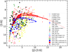 |
Fig. A.1. Colour–magnitude diagram [3.6] vs. [J]–[3.6]. The selected targets for SALT observations are indicated by circles: black (LMC), red (SMC), and green (SK 105). The confirmed post-AGB objects (No. 3, 7, and 11) are plotted as filled circles and are located within 0< [J]–[3.6] < 2 and 12> [3.6]> 14, which may be compared with Fig. 3 of Blum et al. (2006). Object No. 9 has no J photometry. |
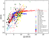 |
Fig. A.2. Colour–magnitude diagram [8.0] vs. [J]-[8.0]. The selected targets for SALT observations are indicated by circles: black (LMC), red (SMC), and green (SK 105). The confirmed post-AGB objects (No. 3, 7, and 11) are plotted as filled circles and are located within 5 < [J]–[8.0] < 7 and 7 > [3.6] > 9, which is located within the extreme AGB star region in Fig. 4 of Blum et al. (2006). Object No. 9 has no J photometry. |
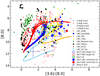 |
Fig. A.3. Colour–magnitude diagram [8.0] vs. [3.6]−[8.0]. The selected targets for SALT observations are indicated by circles: black (LMC), red (SMC), and green (SK 105). The confirmed post-AGB objects (No. 3, 7, 9, and 11) are plotted as filled circles and are located within 3 < [3.6]–[8.0] < 6 and 7 > [8.0] > 9, which can be compared with Fig. 5 of Blum et al. (2006). |
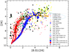 |
Fig. A.4. Colour–magnitude diagram [24.0] vs. [8.0]–[24]. The selected targets for SALT observations are indicated by circles: black (LMC), red (SMC), and green (SK 105). The confirmed post-AGB objects (No. 3, 7, 9, and 11) are plotted as filled circles and are located within 3 < [8.0]–[24] < 5 and 3> [24]> 5, which can be compared with Fig. 6 of Blum et al. (2006). |
All Tables
Designations and positions for the standard star and post-AGB candidates in the Magellanic Clouds.
All Figures
|
Fig. 1. Colour–colour diagram used for the selection of the post-AGB candidates. The main post-AGB candidate area is above the black lines. The numbers in parentheses in the inset list the total number of each class of objects plotted in this figure (see text for details). |
| In the text | |
|
Fig. 2. Red spectra of the objects showing emission lines or emission and absorption lines. The spectra were normalised to continuum. A constant offset of 2.5 was applied between the adjacent spectra. Telluric lines are indicated by wheel cross symbols at the top of the plot. Vertical dashed lines give rest wavelength of the indicated emission lines. For clarity, lines representing Fe II emissions are not described. |
| In the text | |
|
Fig. 3. Spectra of the absorption line or featureless objects in the red setting. The spectra were normalised to continuum. A constant offset of 1.2 was applied between the adjacent spectra. Vertical dashed lines indicate the rest wavelengths of the indicated absorption lines. |
| In the text | |
|
Fig. 4. Spectra of objects in the blue setting. The spectra are normalised to continuum. |
| In the text | |
|
Fig. 5. Synthetic spectrum computed from a model atmosphere without hydrogen (red line), and synthetic spectrum of pure hydrogen atmosphere (green line). The Ca II triplet 8498 Å, 8542 Å, and 8662 Å lines are clearly seen in the red spectrum. The subsequent transitions of the hydrogen Paschen series seen in the green spectrum are indicated in the plot. |
| In the text | |
|
Fig. 6. Best fit of the synthetic spectrum computed for a model atmosphere with effective temperature, gravity, metallicity, and [C/O]: 6500/0.5/−0.5/0.0 (green line) to the observed spectrum of Sk 105 (red line). Arrows indicate the Ca II lines, which are blended with H I Paschen lines. |
| In the text | |
|
Fig. 7. Best fit of the synthetic spectrum computed for a model atmosphere of 6750/0.5/−1.5/0.4 (green line) to the observed spectrum (red line) of object No. 11: J052520. The blue line shows the best solution for the theoretical spectrum computed for model atmospheres with Teff = 9000. |
| In the text | |
|
Fig. 8. Fit to the blue part of spectrum (red line) of object No. 11: J052520 with stellar model parameters derived from the best fit to the red spectrum of this object. The Ca II resonance lines are indicated by arrows. |
| In the text | |
|
Fig. 9. Best fit of the synthetic spectrum computed for a model atmosphere of 6250/0.5/−0.2/0.2 (green line) to the observed spectrum (red line) of object No. 9: J052043. The blue line shows the fit to the observed spectrum with parameters 5750/0.5/−1.0 found by van Aarle et al. (2013). |
| In the text | |
|
Fig. 10. Best fit of the synthetic spectrum computed for a model atmosphere of 6750/0.5/−1.0/0.4 (green line) to the observed spectrum of object No.7: J051110. |
| In the text | |
|
Fig. 11. Best fit of the synthetic spectra computed for model atmospheres of 15 000/2.5/0.0/0.4 (green line) and 10 000/3.0/0.0/0.2 (blue line) to the observed spectrum (red line) of object No. 3 J010546, assuming different continuum levels at 1.0 and 1.03, respectively. |
| In the text | |
|
Fig. 12. Comparison between the spectra of J051110 (red line) and the standard star Sk 105 (green line). Positions of some s-process element transitions are identified on the plot. |
| In the text | |
|
Fig. 13. Best fit of synthetic spectra with enhanced abundances of s-elements to the observed spectra of J051110 (top left), J052043 (top right), J052520 (bottom left), and blue spectrum of J052520 (bottom right). The fit with s-process elements enhanced to the spectrum of J052043 required a reduction in abundances of Ti and Fe of −0.5 dex. |
| In the text | |
|
Fig. 14. Observed spectrum of J05110 (red line) and two fits with enhancement of Ce and no Li (green line), and with both elements enhanced (blue line). See text for more details. The vertical lines show the positions of the Ce II lines. |
| In the text | |
|
Fig. 15. Colour-colour diagram used for selection of the post-AGB candidates (same as in Fig. 1). The main post-AGB candidate area is above the black lines. The grouped class of objects (see text for details) from Jones et al. (2017) are plotted with different symbols. The numbers in parentheses show the total number of each class of object plotted in this figure. |
| In the text | |
|
Fig. A.1. Colour–magnitude diagram [3.6] vs. [J]–[3.6]. The selected targets for SALT observations are indicated by circles: black (LMC), red (SMC), and green (SK 105). The confirmed post-AGB objects (No. 3, 7, and 11) are plotted as filled circles and are located within 0< [J]–[3.6] < 2 and 12> [3.6]> 14, which may be compared with Fig. 3 of Blum et al. (2006). Object No. 9 has no J photometry. |
| In the text | |
|
Fig. A.2. Colour–magnitude diagram [8.0] vs. [J]-[8.0]. The selected targets for SALT observations are indicated by circles: black (LMC), red (SMC), and green (SK 105). The confirmed post-AGB objects (No. 3, 7, and 11) are plotted as filled circles and are located within 5 < [J]–[8.0] < 7 and 7 > [3.6] > 9, which is located within the extreme AGB star region in Fig. 4 of Blum et al. (2006). Object No. 9 has no J photometry. |
| In the text | |
|
Fig. A.3. Colour–magnitude diagram [8.0] vs. [3.6]−[8.0]. The selected targets for SALT observations are indicated by circles: black (LMC), red (SMC), and green (SK 105). The confirmed post-AGB objects (No. 3, 7, 9, and 11) are plotted as filled circles and are located within 3 < [3.6]–[8.0] < 6 and 7 > [8.0] > 9, which can be compared with Fig. 5 of Blum et al. (2006). |
| In the text | |
|
Fig. A.4. Colour–magnitude diagram [24.0] vs. [8.0]–[24]. The selected targets for SALT observations are indicated by circles: black (LMC), red (SMC), and green (SK 105). The confirmed post-AGB objects (No. 3, 7, 9, and 11) are plotted as filled circles and are located within 3 < [8.0]–[24] < 5 and 3> [24]> 5, which can be compared with Fig. 6 of Blum et al. (2006). |
| In the text | |
Current usage metrics show cumulative count of Article Views (full-text article views including HTML views, PDF and ePub downloads, according to the available data) and Abstracts Views on Vision4Press platform.
Data correspond to usage on the plateform after 2015. The current usage metrics is available 48-96 hours after online publication and is updated daily on week days.
Initial download of the metrics may take a while.