| Issue |
A&A
Volume 640, August 2020
|
|
|---|---|---|
| Article Number | A73 | |
| Number of page(s) | 13 | |
| Section | Planets and planetary systems | |
| DOI | https://doi.org/10.1051/0004-6361/202038496 | |
| Published online | 12 August 2020 | |
A significant mutual inclination between the planets within the π Mensae system★
1
European Southern Observatory,
Alonso de Córdova 3107,
Vitacura,
Santiago, Chile
e-mail: This email address is being protected from spambots. You need JavaScript enabled to view it.
2
Department of Astronomy and Astrophysics, Center for Exoplanets and Habitable Worlds, The Pennsylvania State University, University Park,
PA
16802, USA
3
Kavli Institute for Particle Astrophysics and Cosmology, Stanford University,
Stanford,
CA
94305, USA
4
Department of Astronomy, New Mexico State University,
PO Box 30001, MSC 4500,
Las Cruces,
NM
88003, USA
Received:
26
May
2020
Accepted:
16
July
2020
Abstract
Context. Measuring the geometry of multi-planet extrasolar systems can provide insight into their dynamical history and the processes of planetary formation. These types of measurements are challenging for systems that are detected through indirect techniques such as radial velocity and transit, having only been measured for a handful of systems to date.
Aims. We aim to place constraints on the orbital geometry of the outer planet in the π Mensae system, a G0V star at a distance of 18.3 pc that is host to a wide-orbit super-Jovian (M sin i = 10.02 ± 0.15MJup) with a 5.7-yr period and an inner transiting super-Earth (M = 4.82 ± 0.85M⊕) with a 6.3-d period.
Methods. The reflex motion induced by the outer planet on the π Mensae star causes a significant motion of the photocenter of the system on the sky plane over the course of the 5.7-year orbital period of the planet. We combined astrometric measurements from the HIPPARCOS and Gaia satellites with a precisely determined spectroscopic orbit in an attempt to measure this reflex motion, and in turn we constrained the inclination of the orbital plane of the outer planet.
Results. We measure an inclination of ib = 49.9−4.5+5.3 deg for the orbital plane of π Mensae b, leading to a direct measurement of its mass of 13.01−0.95+1.03 MJup. We find a significant mutual inclination between the orbital planes of the two planets, with a 95% credible interval for imut of between 34.°5 and 140.°6 after accounting for the unknown position angle of the orbit of π Mensae c, strongly excluding a co-planar scenario for the two planets within this system. All orbits are stable in the present-day configuration, and secular oscillations of planet c’s eccentricity are quenched by general relativistic precession. Planet c may have undergone high eccentricity tidal migration triggered by Kozai-Lidov cycles, but dynamical histories involving disk migration or in situ formation are not ruled out. Nonetheless, this system provides the first piece of direct evidence that giant planets with large mutual inclinations have a role to play in the origins and evolution of some super-Earth systems.
Key words: astrometry / planets and satellites: dynamical evolution and stability / stars: individual: π Mensae
Tables 5–7 are only available at the CDS via anonymous ftp to cdsarc.u-strasbg.fr (130.79.128.5) or via http://cdsarc.u-strasbg.fr/viz-bin/cat/J/A+A/640/A73
© ESO 2020
1 Introduction
π Mensae (π Men) is a G0V star (Gray et al. 2006) at a distance of 18.2 pc. The star is known to host two planetary-mass companions; a massive super-Jovian with a 5.7-yr period, which was discovered via Doppler spectroscopy (Jones et al. 2002), and a transiting super-Earth with a 6.3-day period (Gandolfi et al. 2018; Huang et al. 2018), which was the first to have been discovered by the Transiting Exoplanet Survey Satellite (TESS; Ricker et al. 2015). Combined radial velocity and transit surveys (Zhu & Wu 2018; Bryan et al. 2019) and the identification of long-period transiting planets (Herman et al. 2019) have shown that these types of system configurations are common; the majority of systems with a long-period gas giant (a > 1 au) also harbor short-period super-Earths (1–4 R⊕), implying potential links between their formation and dynamics. Outer gas giants – particularly those with large eccentricities and/or mutual inclinations – can limit the masses and orbits on which super-Earths form (e.g., Walsh et al. 2011; Childs et al. 2019), stir up their eccentricities and mutual inclinations (e.g., Hansen 2017; Huang et al. 2017; Lai & Pu 2017), drive secular chaos (e.g., Lithwick & Wu 2011), and in extreme cases excite their eccentricities to values that are high enough for tidal migration (e.g., Dawson & Johnson 2018, Sect. 4.4). Masuda et al. (2020) present statistical evidence for a population of high mutual inclination gas giants in systems with single transiting super-Earths; however, due to the limits of the radial velocity and transit techniques, we have yet to directly measure the mutual inclination for any individual systems.
The full orbital characterization of systems containing both outer giant planets and inner super-Earths can also aid our understanding of the origin of short period (<10 day) super-Earths. Similar to hot Jupiters (see Dawson & Johnson 2018 for a review), they may have formed in situ or arrived close to their star via disk or tidal migration. The “Hoptune” population (planets with orbital periods of less than 10 days and sizes between 2 and 6 Earth radii), in particular, exhibits similarities to hot Jupiters in host star metallicity dependence, the lack of other transiting planets in the same system, and occurrence rates (Dong et al. 2018). Dawson & Johnson (2018) argue that high eccentricity tidal migration could account for the fact that these planets did not lose their atmospheres during the star’s young, active stage. Characterizing the full three-dimensional orbital architecture of individual systems containing asuper-Earth accompanied by an outer gas giant can aid us in testing the high eccentricity tidal migration scenario.
The orbital inclination of the outer planet had previously been investigated using HIPPARCOS astrometric measurements of the host star to detect the astrometric reflex motion induced by the planet (Reffert & Quirrenbach 2011). This analysis yielded a plausible range for the orbital inclination of 20.°3–150.°6, corresponding to a maximum mass for the companion of 29.9 MJup. This analysis was not able to conclusively differentiate between a co-planar and a mutually inclined configuration for the system. Efforts have also been made to resolve the outer planet via direct imaging, but the contrast achieved was not sufficient to detect the companion (Zurlo et al. 2018). A single epoch of relative astrometry between the planet and the host star would likely lead to an immediate determination of the inclination of the orbital plane.
In this paper we present an analysis of spectroscopic and astrometric measurements of the motion of the star induced by the orbit of π Men b. We describe the acquisition of the data in Sect. 2. We repeat the analysis presented in Reffert & Quirrenbach (2011) to demonstrate the improvement of the inclination constraints achieved with a revised spectroscopic orbit in Sect. 3. We incorporate the latest astrometric measurements from Gaia into our joint astrometric-spectroscopic model in Sect. 4. We discuss the measured mutual inclination in the context of the dynamical history of the system in Sect. 5, and conclude in Sect. 6.
While this manuscript was being reviewed independent analyses of the same astrometric datasets by Xuan & Wyatt (2020); Damasso et al. (2020) were published. We derive consistent results on the mutual inclination of the two planets despite using a different approach for incorporating the various astrometric measurements of the system.
2 Data acquisition
2.1 Radial velocities
We collected 359 literature and archival radial velocities of the π Men primary star were obtained between 1998 January 16 and 2020 January 8 using the University College London Echelle Spectrograph (UCLES; Diego et al. 1990) and the High Accuracy Radial velocity Planet Searcher (HARPS; Mayor et al. 2003). The 77 velocities from UCLES span from 1998 January 16 until 2015 November 22 (R. Wittenmyer, priv. comm.), the same record used for the discovery and characterization of π Men c (Gandolfi et al. 2018; Huang et al. 2018). The 282 velocities from HARPS span from 2003 December 28 until 2020 January 08 and were obtained from the reduced data products publicly available on the ESO Archive Facility1, an additional seven velocities from HARPS were available but were rejected due to a deterioration of the thorium-argon lamp on 2018 November 26 and 27. The HARPS instrument underwent an intervention on 2015 June 03 that led to a significant change in the radial velocity zero point of the instrument (Lo Curto et al. 2015). To correct for this in our analysis we treated the 129 velocities from before this date as coming from a different instrument (“HARPS1”) to the remaining 153 (“HARPS2”). A complete listing of the radial velocities used in this study is given in Table 5.
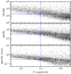 |
Fig. 1 Quality of fit metrics for π Men (yellow cross) and a sample of stars within a factor of two brightness (points) from the Gaia catalog. The parameters shown are the χ2 of the fit of the five-parameter astrometric model to the measurements (top panel), an analog of a reduced χ2 (middle panel), and the sum of the residuals (bottom panel). The quality of the fit for π Men is consistent with that of other stars of a similar brightness. |
2.2 Astrometric data
Astrometric measurements of the π Men systemwere obtained from HIPPARCOS catalog re-reduction (van Leeuwen 2007a) and from the second Gaia data release (DR2; Gaia Collaboration 2018). The coordinates are expressed in the ICRS reference frame at the 1991.25 epoch for HIPPARCOS and the 2015.5 epoch for Gaia. A minor correction to the Gaia astrometry was applied to account for the orientation and rotation of the bright star reference (for π Men: Δα⋆ = −1.37 ± 0.34 mas, Δδ = 0.15 ± 0.16 mas,  mas yr−1; Lindegren et al. 2018; Lindegren 2019)2, and the ~10% error inflation terms des- cribed in Arenou et al. (2018). We used the revised orientation and spin parameters presented in Lindegren (2020); ɛX = − 0.019 ±0.158 mas, ɛY = 1.304 ± 0.349 mas, ɛZ = 0.553 ± 0.135 mas, ωX = −0.068 ± 0.052 mas yr−1, ωY = −0.051 ± 0.045 mas yr−1, ωZ = −0.014 ± 0.066 mas yr−1), applying them to the catalog values using a Monte Carlo-based approach. The goodness of fit metrics given in the Gaia catalog are better than for a typical star of a similar magnitude (Fig. 1). The astrometric measurements from both catalogs, after applying the correction for the Gaia values, are given in Table 1.
In addition to the HIPPARCOS catalog values, we also obtained the individual measurements made by the satellite of π Men that were used toderive the five astrometric parameters given in Table 1. These measurements are effectively one-dimensional, constrainingthe position of the star to within 1–2 mas along a great circle on the celestial sphere with a scan orientation angle ψ (a north-south scan has ψ = π∕2). Instead of publishing the abscissa data Λ – the raw scan measurements – the re-reduction of the HIPPARCOS data presented the abscissa residuals δΛ after the best-fit astrometric model had been subtracted. These are referred to as the HIPPARCOS intermediate astrometric data (IAD; van Leeuwen 2007b).
The IAD for π Men contain the epoch t, parallax factor Π, scan orientation ψ, abscissa residual δΛ and corresponding uncertainty σΛ for each of the 137 measurements of the star (Table 6). The measurements span from 1989 November 05 until 1993 January 29, have an average uncertainty of 1.6 mas, and none were rejected when fitting the astrometric model presented in the catalog. The abscissa ΛHIP can be reconstructed using the formalism described in Sahlmann et al. (2011) as
 (1)
(1)
We also decomposed four of the astrometric parameters into a constant term and an offset (e.g.,  ) to avoid precision loss. When reconstructing the abscissa both the constant and offset terms were set to zero:
 (2)
(2)
which we can compare to a noiseless model abscissa generated with a small perturbation of the catalog parameters
 (3)
(3)
in order to compute a goodness of fit, for example.
The individual scan measurements from the Gaia satellite are only due to be published at the conclusion of the mission, limiting us to the astrometric parameters presented in the catalog. However, the predicted date, parallax factor, and scan orientation θ of the individual Gaia measurements are available3 (Table 7), giving us the necessary information to perform a simplistic simulation of the Gaia measurement of the position and motion of the photocenter. Unlike for HIPPARCOS, here the scan orientation describes the position angle of the scan direction relative to north4 (i.e., a north-south scan has θ = 0). These simulated measurements can be compared with the catalog values to constrain the photocenter motion during the time span of the Gaia measurements. We generated a forecast using this tool on 2020 January 7, resulting in a prediction of 26 measurements between 2014 August 26 and 2016 May 20, within the range of dates for which measurements were used to constructthe DR2 catalog. This is more than the 21 transits used to compute the astrometric parameters in the catalog, consistent with the warning on the gost utility website that only 80% of the measurements are usable.
Astrometric measurements of the photocenter of the π Mensae system.
3 Photocenter motion measured by HIPPARCOS
The presence of a massive companion to π Men makes interpretation of astrometric measurements of this object more challenging. In a single star system the barycenter and photocenter of the system are coincident with the location of the star. In an unresolved multiple system with two or more objects of unequal brightness – as is the case for the π Men system – the photocenter, barycenter, and the location of the primary star are no longer coincident. Astrometric measurements of this type of system are therefore of the position and motion of the photocenter of the system, a combination of the constant velocity of the system barycenter through space and the orbital motion of the photocenter around the barycenter.
We first investigated whether a combination of the HIPPARCOS IAD and the best fit spectroscopic orbit can provide any significant constraint on the geometry of the orbit of π Men b. We implemented the grid-based approach presented in Sahlmann et al. (2011) where for each combination of the orbital inclination i and longitude of the ascending node5 Ω, the orbital elements measured from the spectroscopic orbit were fixed, and the astrometric parameters were calculated using a least-squares based approach.
3.1 Model description
A Keplerian fit to the radial velocities provides a measurement of the period P, velocity semi-amplitude K1, eccentricity e, argument of periastron ω⋆ and the time of periastron T0 of the orbit of the star around the system barycenter. Here we use the notation ω⋆ to refer to the argument of periastron for the primary star, and ω = ω⋆ + π as the argument of periastron for the companion. These spectroscopic elements can be combined with an assumed mass of the primary star M1 and the inclination of the orbit i to determine the mass ratio q = M2∕M1 by solving the following expression for the mass function
 (4)
(4)
where G is the gravitational constant. The total semi-major axis a in astronomical units can then be calculated using Kepler’s third law as
 (5)
(5)
when the period and masses are expressed in years and solar masses.
The semi-major axis of the photocenter orbit ap around the barycenter of a binary system can be calculated from the total semi-major axis of the orbit a, the masses of the two components M1 and M2, and their magnitude difference Δm = − 2.5 log(F2∕F1). We define the fractional mass B as
 (6)
(6)
and the analogous fractional flux β as
 (7)
(7)
from which ap can be calculated as  (e.g., Heintz 1978; Coughlin & López-Morales 2012). In a binary system where the companion is much fainter than the primary star, the value of β asymptotes to zero and the photocenter orbit can be considered as coincident with the orbit of the primary around the barycenter (i.e., ap ≈ a1). We include this term for completeness; it is only relevant for extremely low inclinations where the mass of the secondary exceeds the hydrogen burning limit. The value of β is almost always wavelength dependent unless the spectral energy distributions of the two objects are identical. We refer to fractional fluxes computed using the HIPPARCOS Hp filter as βH, and those using the Gaia G filter as βG. We used an empirical mass-magnitude relationship for stars to determine the flux ratio for solutions where M2 > 0.077M⊙ (Pecaut & Mamajek 2013), and set βH = βG = 0 otherwise.
The position of the photocenter relative to the barycenter in the sky plane can be calculated from the elements discussed previously, the position angle of the ascending node Ω and the epoch of the observation. The radius of a photocenter orbit rp at a given epoch is defined as
 (8)
(8)
where the true anomaly ν is computed from the mean and eccentric anomalies M and E
 (9)
(9)
The offset between the photocenter and barycenter in the right ascension x and declination y directions can be calculated as
![Mathematical equation: \begin{equation*} \begin{split} \hspace*{-2pt}x &\,{=}\, r_{\textrm{p}}\left[\cos\left(\omega_{\star} + \nu \right)\sin\Omega + \sin\left(\omega_{\star} + \nu \right)\cos\Omega\cos i\right], \\ \hspace*{-2pt}y &\,{=}\, r_{\textrm{p}}\left[\cos\left(\omega_{\star} + \nu \right)\cos\Omega - \sin\left(\omega_{\star} + \nu \right)\sin\Omega\cos i\right]. \\ \end{split} \end{equation*}](/articles/aa/full_html/2020/08/aa38496-20/aa38496-20-eq15.png) (10)
(10)
We modeled a HIPPARCOS abscissa by combining the five standard astrometric parameters described previously with the motion of the photocenter in the right ascension and declination directions. As in Sahlmann et al. (2011) we defined a new variable
 (11)
(11)
that converts the two-dimensional measurement into a one-dimensional measurement along the orientation of the scan. This variable is expressed in astronomical units, allowing us to account for a potential change in the best fit parallax of the star. We combined this new variable with our model abscissa given in Eq. (3) as
 (12)
(12)
The least-squares solution to this linear equation can be found numerically via a matrix-based approach:
 (13)
(13)
where A is a (5, 137) matrix constructed using the values from the HIPPARCOS IAD and the variable ϒ defined previously;
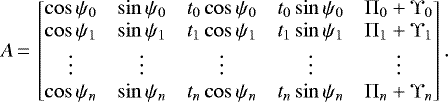 (14)
(14)
The least-squares solution can be used to construct a model abscissa using Eq. (12) which can be compared with the reconstructed HIPPARCOS abscissa to calculate the goodness of fit
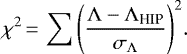 (15)
(15)
This calculation was performed on a finely sampled i-Ω grid, with 500 elements between i = 0 deg and 180 deg and 1000 elements between Ω = 0 deg and 360 deg.
3.2 Model validation
We verified our model implementation by comparing to the results of a previous study combining radial velocity and HIPPARCOS measurements by Reffert & Quirrenbach (2011). We first applied it to HD 168443, a brown dwarf with a minimum mass of M sin i = 18MJup on a 4.8 yr orbit. To ensure consistency with the previous study we used the same spectroscopic orbital elements from Butler et al. (2006). We found  at i = 36.°1 Ω = 131.°1 and a 3σ range for i of 17.°8–163.°0, consistent with their results for this system. Our χ2 surface for this example is a good match to their Fig. 3. We found similarly consistent results for other systems in their study.
3.3 Application to π Mensae
We first applied this model to π Men using the spectroscopic orbital elements from Butler et al. (2006) both to compare with previous results from Reffert & Quirrenbach (2011) and to demonstrate the effect of a revised spectroscopic orbit on the determination of the astrometric orbit of the photocenter. With data spanning slightly more than one orbital period, Butler et al. (2006) measured P = 2151 d, K1 = 196.4 m s−1, e = 0.6405, ω⋆ = 330.°24 and T0 = 47819.5 MJD. We used these spectroscopic elements and their estimate for the mass of the primary of 1.1M⊙. We used the same size and range for the i-Ω grid described previously. The small subset of inclinations that correspond to orbital configurations where M2 > M1 are ignored by setting χ2 = ∞.
The resulting χ2 surface is shown in Fig. 2 (left panel). We found a minimum χ2 of 198.0 at i = 55.°6 and Ω = 219.°5 ( given 137 measurements and five free parameters), with marginalized 1σ confidence intervals of 49.°6–99.°2 for i and 180.°5–248.°6 for Ω. The minimum χ2 is a slight improvement over the single star five-parameter astrometric model (
 ,
,  ), however the reduced χ2 in both cases suggests a slight underestimate in the HIPPARCOS abscissa uncertainties. Our results are consistent with the 3σ joint confidence interval on the inclination in Reffert & Quirrenbach (2011); we found a range of 21.°4–144.°6, compared to 20.°3–150.°6 within their study.
This technique is dependent on having a good estimate of the motion of the photocenter of the system during time span of the HIPPARCOS observations. The radial velocity record used by Butler et al. (2006) covered one and a third orbital periods, but only sampled the part of the orbit with the maximum velocity change near periastron once. This resulted in quite a large uncertainty in the period (σP = 85 d) which translated into an uncertainty of the epoch of periastron in late 1989/early 1990 of  d. This causes significant uncertainty in the model of the astrometric motion of the photocenter for a given M1, i, and Ω.
We used the radial velocity record that we compiled (Sect. 2.1) to revise the measurements of the spectroscopic orbital elements. We used maximum likelihood estimation to determine the Keplerian orbit that best fit the data. The radial velocity of the star v is calculated from the spectroscopic orbital elements as
![Mathematical equation: \begin{equation*} v\,{=}\,K_1\left[e\cos\omega_{\star}+ \cos\left(\nu + \omega_{\star}\right)\right] + \gamma. \end{equation*}](/articles/aa/full_html/2020/08/aa38496-20/aa38496-20-eq26.png) (16)
(16)
Here γ is the time-dependent apparent radial velocity of the system barycenter; secular acceleration due to the changing perspective between us an the π Mensae system cause a significant change in the apparent radial velocity of the barycenter, which is assumed to be moving linearly through space, over the twenty-year radial velocity record. We used the coordinate transformations described in Butkevich & Lindegren (2014) and the HIPPARCOS astrometry in Table 1 to account for this effect (see also Sect. 4.1). We evaluated the likelihood  using the predicted velocities derived from of a given set of orbital parameters as
![Mathematical equation: \begin{align*} \ln \mathcal{L}_i\,{=}&\,{-}\frac{1}{2} \sum_j^{n_i}\left[\frac{\left(v_j^{\textrm{model}} - \left[v_j^{\textrm{obs}}+\Delta v_i\right]\right)^2}{\sigma^2_j + \epsilon_i^2}+ \ln \left(2\pi\left[\sigma^2_j + \epsilon^2_i\right]\right)\vphantom{\frac{\left(v_j^{\textrm{model}} - \left[v_j^{\textrm{obs}}+\Delta v_i\right]\right)^2}{\sigma^2_j + \epsilon_i^2}}\right], \end{align*}](/articles/aa/full_html/2020/08/aa38496-20/aa38496-20-eq28.png) (17)
(17)
where  and
and  are the predicted and measured velocities for the jth epoch, and σj is the uncertainty of the measurement. The likelihood was evaluated for each instrument i independently. The summation was performed over the ni measurements for the ith instrument, with two additional terms describing the radial velocity offset for that instrument Δvi, and an error inflation term ɛi to account for both underestimated uncertainties and stellar jitter (e.g., Price-Whelan et al. 2017; Fulton et al. 2018). The final likelihood was then calculated as
  . We used the HARPS measurements taken prior to the replacement of the fibers (“HARPS1”) to define our absolute radial velocity zero-point by fixing Δvi to zero for this instrument.
Table 2 contains the maximum likelihood estimate of the set of spectroscopic orbital elements for the orbit of π Men b. We used a typical parameterization for the spectroscopic elements where the eccentricity e and argument of periastron ω⋆ are combined into  and
and  to avoid angle wrapping. The effect of the inner planet on these orbital parameters is negligible due to the significantly smaller velocity semi-amplitude and shorter orbital period. We repeated the analysis of the HIPPARCOS IAD using this updated set of orbital elements. Here we used the mass estimate of M1 = 1.094 ± 0.039M⊙ from Huang et al. (2018). The resulting χ2 surface is shown in Fig. 2 (right panel), showing a significant improvement of the constraint of the inclination of the orbit. We found a minimum χ2 of 193.4 at i = 45.°1 and Ω = 253.°0 (
 ), an improved goodness of fit with the more accurate model of the photocenter motion during the time span of the HIPPARCOS measurements. The marginalized 1σ confidence intervals for i and Ω are 37.°6–66.°0 and 237.°5–269.°2. An edge-on orbit of i ~ 90 deg for π Men b is weakly excluded when only using the HIPPARCOS IAD at the ~1.5σ level.
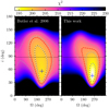 |
Fig. 2 Goodness of fit (χ2) as a functionof the inclination i and the position angle of the ascending node Ω for the photocenter orbit of the π Men system using the spectroscopic orbit from Butler et al. (2006; left), and the revised orbit presented in Table 2 (right). Dashed lines (black and white) denote areas enclosing 68, 95, and 99.7% of the probability. The value of
|

Maximum likelihood estimate of the spectroscopic orbit of π Mensae b.
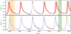 |
Fig. 3 Spectroscopic orbit of the star π Men aroundthe system barycenter using the radial velocity record presented in Butler et al. (2006; top panel) and this work (bottom panel). Measurements are plotted from UCLES (black circles), HARPS1 (pre-upgrade, pink squares), and HARPS2 (post-upgrade; yellow diamonds). The maximum likelihood orbit is plotted as a dashed line, with draws from an MCMC fit shown as light solid lines. The orbit is now so well constrained that the uncertainty of the predicted radial velocity at any given epoch is smaller than the thickness of the dashed line. In both panels the best fit orbit computed by Butler et al. (2006) and used by Reffert & Quirrenbach (2011) is shown as a solid gray curve. Dates of the individual HIPPARCOS and Gaia measurements are denoted by orange and green vertical lines, respectively. |
4 Incorporating Gaia astrometry
Astrometric measurements of bright stars such as π Men with Gaia have a typical per-scan measurement error of ~1 mas, comparable to that achieved with HIPPARCOS, and worse than predicted from models of the instrument (Lindegren et al. 2018). Despite this, the combination of two extremely precise measurements of the photocenter location separated by approximately 24 yr, the HIPPARCOS IAD and the instantaneous proper motion measured by Gaia can be used to measure deviations from linear motion caused by the presence of an orbiting companion (e.g., Kervella et al. 2019).
Without access to the individual astrometric measurements used to fit the astrometric parameters given within the catalog it is not possible to perform the same analysis as applied to the HIPPARCOS data described in Sect. 3. Instead, we used the predicted scan timings, orientations, and parallax factors to forward model the Gaia measurement of the position and motion of the photocenter at the Gaia reference epoch of 2015.5. This method will be most reliable with a relatively constant photocenter motion over the time span of the Gaia scans of the star, with only a small deviation from linear motion. The Gaia scans of π Men are sampling a relatively slow part of the orbit (Fig. 3, bottom panel), with a constant rate of astrometric acceleration of ~1 mas yr−2 predicted from the best fit orbit from Sect. 3, depending on the orbital inclination. This is comparable in magnitude to the very smallest accelerations detected by HIPPARCOS with a longer baseline of observations; 99% of the stars where the accelerating model was a better fit than the linear motion model had accelerations of > 1.6 mas yr−2. The relatively constant motion of the photocenter also mitigates the effect of the discrepancy between the number of predicted scans (26) and the actual number of scans used in the Gaia catalog (21) as described in Sect. 2.2, especially if these five missing scans are randomly distributed throughout the time span of the Gaia measurements. The upcoming Gaia data releases will contain measurements of astrometric accelerations where appropriate with which it will be possible for a more precise simulation of the Gaia measurement without access to the individual measurements themselves.
4.1 Model description
The model was adapted from the one used in De Rosa et al. (2019) to handle radial velocity data from multiple instruments and the lack of any relevant direct imaging constraints for this system. The model consists of twenty parameters that allow us to connect our physical model of the system to the astrometric and spectroscopic observations. These parameters are described in Table 3. In this model the barycenter of the π Men system in 1991.25 is located at
 (18)
(18)
with a parallax and proper motion of
 (19)
(19)
where the H subscript denotes values from the HIPPARCOS catalog. We followed the same procedure described in Sect. 3 to generate a model HIPPARCOS abscissa Λ using the parallax ϖ, the offsets to the remaining four astrometric parameters, and the variable ϒ that encodes the photocenter motion for a given set of orbital parameters. The likelihood of the set of model parameters given the HIPPARCOS measurements was evaluated as
![Mathematical equation: \begin{equation*} \ln \mathcal{L_{\textrm{H}}}\,{=}\,{-}\frac{1}{2}\sum\left[\frac{\left(\Lambda - \Lambda_{\textrm{HIP}}\right)^2}{\sigma_{\Lambda}^2 + \epsilon_{\textrm{HIP}}^2} + \ln \left(2\pi\left[\sigma_{\Lambda}^2 + \epsilon_{\textrm{HIP}}^2\right]\right)\right]. \end{equation*}](/articles/aa/full_html/2020/08/aa38496-20/aa38496-20-eq37.png) (20)
(20)
The error inflation term ɛHIP was added to account for the apparent underestimation of the HIPPARCOS IAD uncertainties noted in Sect. 3.3.
The π Men barycenter was then propagated from the HIPPARCOS reference epoch (J1991.25) to the Gaia reference epoch (J2015.5) using the rigorous coordinate transformation procedure described in Butkevich & Lindegren (2014). This procedure propagates the spherical coordinates, parallax, and tangent-plane proper motions, accounting for the non-rectilinear nature of the ICRS coordinate system. This transformation is critical given the declination of the star; applying the simplistic transformation using the tangent plane approximation would result in a 2.9 mas error in the position and a 0.2 mas yr−1 error in the proper motion of the star at the Gaia reference epoch, mimicking photocenter motion due to the orbiting companion. This coordinate transform also accounts for the secular acceleration of the radial velocity of the system barycenter. As in Sect. 3.3, we fit for the apparent radial velocity of the system barycenter at 1991.25 (γ1991.25).
With the barycenter propagated to 2015.5, we simulated the motion of the photocenter during the time span of the Gaia measurements using the propagated parallax and proper motions, and the predicted photocenter motion caused by the orbiting companion. The photocenter orbit semi-major axis was calculated using βG due to the differing filter responses of HIPPARCOS and Gaia. We then performed a simple least-squares fit to the motion of the star to simulate theGaia measurement of the five astrometric parameters presented in the catalog using the scan timings, angles, and parallax factors obtained from the gost utility described previously. We constructed a residual vector r containing the difference between the catalog and simulated position and proper motion measurements. This was used to calculate the likelihood of the model parameters given the Gaia measurements as
 (21)
(21)
where C is the covariance matrix of the Gaia catalog measurements constructed using the uncertainties and relevant correlation coefficients.
The likelihood of the model parameters given the radial velocity measurements was calculated as in Sect. 3.3
 (22)
(22)
for each of the n instruments used to construct the radial velocity record in Table 5. The final likelihood was calculated by summing the three components
 (23)
(23)
Joint astrometric-spectroscopic model parameters.
4.2 Application to π Mensae
We used a combination of maximum likelihood estimation and Markov chain Monte Carlo (MCMC) to determine the best fit model parameters and their uncertainties and covariances given the astrometric and spectroscopic measurements of the π Men system. This was performed with four combinations of the astrometric data; HIPPARCOS only to compare with the results in Sect. 3, and with the various combinations of the HIPPARCOS and the Gaia position and proper motion measurements. The maximum likelihood parameter set was found using the Nelder-Mead simplex algorithm within the scipy.optimize package (Virtanen et al. 2020). We fixed M1 = 1.094M⊙ for this step as this parameter is not constrained by any of the measurements. The results for each of the four combinations of astrometric data are listed in Table 4.
The uncertainties on the model parameters were estimated using a Markov chain Monte Carlo algorithm. We used the parallel-tempering affine-invariant sampler emcee (Foreman-Mackey et al. 2013) to thoroughly explore the posterior distributions of each parameter. We initialized 512 MCMC chains at each of 16 “temperatures” (a total of 8192 chains) near the best fit solution identified via the maximum likelihood analysis described previously. The lowest temperature chains for parallel-tempering MCMC explore the posterior distribution of each parameter, whilst the highest temperature chains explore the priors. This is especially advantageous for complex likelihood volumes to ensure parameter space is fully explored.
Each chain was advanced by 105 steps with every tenth step saved to disk. At each step a probability was calculated by combining the likelihood from Eq. (23) with the prior probabilities given the distributions listed in Table 3. We discarded the first fifth of the chain as “burn-in” where the chain positions were still a function of their initial conditions. While we did not apply a statistical check for convergence, the chains appeared well-mixed based on a visual inspection of the chain position as a function of step number, with the median and 1σ ranges of each parameter not significantly changing. This process was repeated for each of the four combinations of astrometric data. The resulting median and 1σ credible intervals are given in Table 4 for the twenty fitted parameters, along with several derived parameters. A visualization of the fit using all of the available astrometric data is shown in Fig. 4. We found  for the maximum likelihood estimate of the fit using all of the astrometry available given the 500 measurements and 20 model parameters, but this parameter is dominated by the goodness of fit to the radial velocity measurements and the HIPPARCOS IAD. The quality of the fit to the Gaia measurements is good, although there is some tension between the prediction and measurement of the photocenter proper motion in the declination direction (Fig. 4). A potential source of this discrepancy is a residual systematic rotation of the bright star reference frame not corrected using the model from Lindegren (2019, 2020).
Maximum likelihood estimate and MCMC median and 1σ credible intervals for the fitted and derived parameters.
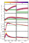 |
Fig. 4 Position (top two panels) and proper motion (bottom two panels) of the photocenter during time span of the HIPPARCOS and Gaia measurements used in this study from the fit using all available astrometric data. For the position plots the proper motion of the barycenter was subtracted, and the positions are relative to the catalog values. The position of the barycenter relative to the catalog value and its proper motion are also plotted (horizontal green lines). The significant change in the proper motion of the barycenter in the α⋆ direction is due to the southern declination of the star. catalog values are plotted as the circle with thick error bars. Simulated measurements based on a five-parameter fit to the combined motion of the photocenter and barycenter are shown by the more extended error bars. |
4.3 Independent analysis
In order to further verify these results, we performed a second analysis with an independent fitting routine for joint astrometry and RV fits, as previously used in Nielsen et al. (2020) for the directly-imaged planet β Pictoris b. This routine was modified for π Men b, fitting for 20 parameters, including the standard set of seven for visual orbits: semi-major axis (a), eccentricity (e), inclination angle (i), argument of periastron of the planet (ω), position angle of the ascending (Ω), epoch of periastron passage (T0), and period (P). Also fitted were seven radial velocity parameters, including system radial velocity at 1991.25 (γ1991.25), m sin i of the secondary, RV offsets (ΔvH2, ΔvU), and jitter terms for each instrument, ɛH1, ɛH2, and ɛU, as well as the error inflation term for the HIPPARCOS abscissa data ɛHIP. Finally, the five astrometric parameters; the offset of the photocenter from the HIPPARCOS catalog position of π Men at 1991.25 (Δα⋆, Δδ), parallax (ϖ), and proper motion at 1991.25 ( , μδ). We assumed priors that are uniform in loga, log P, cos i, and uniform in all other parameters, except for an additional prior on the derived mass of the primary (M1), as above taken to be a Gaussian with mean of 1.094 M⊙ and σ of 0.039 M⊙. As above, we utilized the full RV dataset for π Men, and the Gaia DR2 position and proper motion measurements and errors. However, we used a separate method to convert the hipparcos IAD residuals and scan directions into individual measurements, as in Nielsen et al. (2020). Unlike Nielsen et al. (2020), we used rigorous propagation of position and proper motion from 1991.25 to 2015.5, by transforming position, proper motion, radial velocity, and parallax from angular coordinate to Cartesian, update all six values assuming linear motion, then transform back to angular coordinates. Fitting is then done using a Metropolis-Hastings MCMC routine.
Despite the different method we found very similar results to the HIPPARCOS, Gaia, position and proper motion fit given in Table 4. This second method finds value of [semi-major axis, period, eccentricity, position angle of nodes, argument of periastron of the star, secondary mass, inclination angle] of [ au,
au,  , 0.6438 ± 0.0015,
  , 330.58 ± 0.31°,
  MJup,
MJup,  ], compared to the values aboveof [3.308 ± 0.039 au,
  d, 0.6450 ± 0.0011,
  ,
,  ,
,  MJup,
MJup,  ]. For all parameters, the medians and confidence intervals are almost identical from the two methods. This gives us further confidence in the measurement of the parameter most of interest, inclination angle, which is essentially the same for the two orbit-fitting methods.
4.4 Mutual inclination
The joint fit of the spectroscopic and all of the astrometric measurements yielded an inclination of  deg and a position angle of the ascending node of
  deg for the orbit of π Men b (Fig. 5). We found consistent values for these parameters for each of the four fitsshown in Table 4. This inclination corresponds to a mass of π Men b of
  MJup, a mass straddling the deuterium-burning limit sometimes used as the planet-brown dwarf boundary. The mutual inclination imut between the orbital plane of the two planets in this system cannot be directly measured as the position angle of the orbit of π Men c (Ωc) is currently unconstrained.
We instead estimated a plausible range of the mutual inclination assuming that the position angle of theorbit of the inner planet is randomly oriented relative to that of the outer planet,  . We estimated the posterior distribution of imut by combining the posterior distributions for the inclination and position angle for π Men b (ib, Ωb) calculated previously, the inclination for π Men c (
 deg; Huang et al. 2018, although an inclination of 180 − ic is also consistent with the transit observations), and our assumption for the posterior distribution of Ωc ;
 (24)
(24)
This yielded a 95th-percentile lower limit on the mutual inclination of imut > 34.°5 given our assumption for p(Ωc). The probability density function of the value of imut is shown in Fig. 6, alongside the prior probability density function to demonstrate the constraints provided by the measurements. The minimum value of imut from the 4 096 000 samples was 7.°4. We adopted the 95th-percentile credible interval of imut from 34.°5 to 140.°6 as the range of plausible mutual inclinations for the system given the observational data. We found a similar lower limit of imut > 30.°2 when assuming Ωb = Ωc, indicating that the lower limit of this value is not strongly affected by the assumption made regarding the value of Ωc. A co-planar configuration for the two planets in the π Men system is strongly excluded based on the spectroscopic and astrometric measurements used within this analysis.
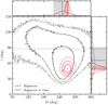 |
Fig. 5 Covariance between the position angle of the ascending node Ω and inclination i, and corresponding marginalized distributions, of the photocenter orbit of the π Men system from the MCMC calculation using only the HIPPARCOS measurements (black) and using all available astrometry (red). Contours denote areas encompassing 68, 95, and 99.7% of the probability. Marginalized 1σ credible intervals are indicated. The values of i and Ω from the maximum likelihood analyses are shown for reference (cross symbols). The orbital inclination of π Men b is significantly different from that of the inner planet (blue dotted line), indicating that the system is not aligned. |
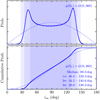 |
Fig. 6 Posterior probability (top) and cumulative (bottom) distribution for the value of imut under the assumption that |

5 Dynamical constraints on present-day orbit and dynamical history
On its current orbit, the inner planet π Men c is shielded by general relativistic precession from strong dynamical perturbations by π Men b. Therefore a long-term stability requirement does not place any additional constraints on π Men b’s orbital properties. We simulated the system at a range of mutual inclinations by approximating planet c as a test particle and solving Lagrange’s equations of motion using a secular disturbing potential expanded to octupolar order (Yokoyama et al. 2003), including general relativistic precession of both planets’ orbits. Including the octupolar order is particularly important for this nearby, eccentric outer planet (e.g., Ford et al. 2000; Naoz et al. 2011; Teyssandier et al. 2013; Li et al. 2014). We set planet c’s initial eccentricity to 0 and used the mass and orbit of planet b from Table 4. For the entire range of possible mutual inclinations, the system remained stable: planet c’s eccentricity is not excited to a value high enough for tidal disruption (Fig. 7). π Men c’s present-day semi-major axis is close to the value at which general relativistic precession prevents π Men b from exciting its eccentricity above 0.1 (Fig. 8).
π Men c may have undergone high eccentricity tidal migration (e.g., Hut 1981) to reach its present day short orbital period. In one version of this scenario, planets b and c form on or migrate to well-separated orbits. On a stable orbit, planet c must reside closer to the star than 0.69 au (Petrovich 2015a). π Men b is disturbed toits observed high eccentricity, perhaps by scattering or ejecting another planet (e.g., Jurić & Tremaine 2008). This disturbance creates a sufficient mutual inclination between planets b and c (e.g., Chatterjee et al. 2008) to trigger Kozai-Lidov cycles (e.g., Kozai 1962; Lidov 1962; Naoz 2016), raising planet c’s eccentricity and triggering high eccentricity tidal migration.
Figure 9 shows an example of this first scenario. We included tidal evolution following Wu & Murray (2003) with a tidal quality factor Qp = 103 and initial mutual inclination of 45 degrees, eccentricity of 0, and semi-major of 0.2 au for π Men c, resulting in a mutual final inclination of 38.5°. If planet c originally had its eccentricity excited by Kozai-Lidov cycles, underwent significant tidal migration, and is fully tidally circularized today, we expect to observe it at mutual inclination near ~ 40° or ~ 140° (e.g., Fabrycky & Tremaine 2007; Petrovich & Tremaine 2016). Much lower present-day mutual inclinations (i.e., closer to 0 and 180) are possible if planet c began with a large eccentricity. For example, in an initially coplanar configuration where planet b has an initial eccentricity of 0.45, longitude of periapse opposite planet b, and semi-major of 0.45 au, the final mutual inclination is 10°.
However, we cannot assume that planet c has completed its tidal circularization. Its observed eccentricity is not well constrained by the radial-velocity or transit light curve datasets (Huang et al. 2018; Gandolfi et al. 2018), and other mini-Neptunes at short orbital periods have retained their orbital eccentricities (e.g., GJ 436b, Maness et al. 2007). Their tidal quality factors are not well known, with values of Qp spanning 102 –106 (or an even wider range) quite plausible. We might observe a higher mutual inclination (i.e., much closer to polar than ~ 40 or 140°) if planet c is still in the process of tidally circularizing and has not migrated a substantial distance. For example, planet c could have started at a = 0.1 au and e = 0 and mutual inclination of 65°, been excited by Kozai-Lidov cycles onto an orbit with a periapse several times the Roche limit, experienced rather weak tidal dissipation with Qp = 107, and arrived to its present-day semi-major axis after 1 Gyr with e oscillating between 0.6 and 0.75 and mutual inclination oscillating between 54 and 63° as it continues ongoing tidal evolution. At larger initial semi-major axes, near polar mutual inclinations lead to either close periapse passages that result in tidal disruption or quick tidal circularization to semi-major axes much smaller than planet c’s current semi-major axis.
Another variation on the tidal migration scenario is that π Men c underwenthigh eccentricity migration initially triggered by planet-planet scattering (e.g., Rasio & Ford 1996) or secular chaos (e.g., Wu & Lithwick 2011) rather than planet-planet Kozai-Lidov cycles. This scenario does not require a particular mutual inclination. The evolution could involve Kozai-Lidov cycles – or coplanar secular eccentricity cycles (e.g., Petrovich 2015b) – once tidal evolution separates the planets.
Another possibility is that π Men c formed at or near its current location (e.g., Lee et al. 2014), or arrived via disk migration (e.g., Cossou et al. 2014). As described above, general relativistic precession mostly decouples it from planet b, with modest oscillations in eccentricity and inclination. Planet c may even reside in a close-in multi-planet system (which would not be easily compatible with the high eccentricity migration scenario above); radial velocity and transit timing constraints do not rule out the presence of other small planets. Depending on their spacing, coupling among the inner planets may cause them to oscillate in inclination together as a coplanar set, slightly excite their mutual inclinations (e.g., Lai & Pu 2017; Huang et al. 2017; Masuda et al. 2020; our Fig. 10), or even allow for a modest eccentricity excitation that results in short scale tidal migration of planet c. The detection of other planets in the system could allow for stronger stability constraints on mutual inclinations.
Therefore a variety of origins scenarios are consistent with the system’s known properties. The significant mutual inclination makes the high eccentricity migration scenario appealing and the most likely observed mutual inclinations coincide with those expected from high eccentricity tidal migration with planet c’s eccentricity originally excited by Kozai-Lidov cycles. Moreover, with a radius of 2.04 R⊕ (Huang et al. 2018) and period of 6.27 days, π Men c is a member population of short period, 2–6 R⊕ planets identified by Dong et al. (2018), which Dawson & Johnson (2018) argue are likely to have undergone high eccentricity tidal migration. However, we cannot rule out a quieter history involving in situ formation or disk migration. Crucially, this system provides thefirst direct measurement of a mutually inclined outer giant posited for a variety of super-Earth formation and evolution histories.
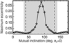 |
Fig. 7 Maximum eccentricity of π Men c excited by secular effects of π Men b over 2.7 Gyr as a function of semi-major axis. We assume an initial eccentricity of 0 for π Men c. π Men c is shielded by general relativistic precession from strong dynamical perturbations by π Men b. The shaded region indicates the 95% confidence interval on the observed imut and the dashed lines indicate the most likely values. |
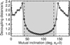 |
Fig. 8 Decoupling distance: semi-major axis of π Men c for which general relativistic precession prevents π Men b from exciting its eccentricity above 0.1. We assume an initial eccentricity of 0 for π Men c. Dotted horizontal line: π Men c’s present-day semi-major axis. The shaded region indicates the 95% confidence interval on the observed imut and the dashed lines indicate the most likely values. |
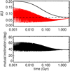 |
Fig. 9 Example of high eccentricity Kozai-Lidov tidal migration scenario. Top: evolution of π Men c’s semi-major axis (black) and periapse (red). Bottom panel: mutual inclination. π Men c circularizes to its present-day semi-major axis with a mutual inclination of 38.5°. |
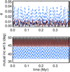 |
Fig. 10 Example behavior of multi-planet system, with π Men c (black solid) at its present-day semi-major axis, two other planets of the same mass located at 0.103 au (red dotted) and 0.185 au (blue dashed), and π Men b. Perturbations from planet b lead to modest eccentricities (top panel) and mutual inclinations among the planets (bottom panel; i.e., each planet has a slightly different mutual inclination with planet b). Dynamical evolution computed in mercury6. Chambers (1999), modified to include general relativistic precession of all planets. |
6 Conclusion
We have presented a joint analysis of spectroscopic and astrometric measurements of the motion of the planet-hosting star π Mensae induced by the massive ( MJup) planet π Mensae b orbiting with a period of 5.7 yr. This analysis yielded a direct measurement of the inclination of the orbital plane of the outer planet of
  deg, strongly excluding a co-planar configuration with the inner transiting super-Earth. The mutual inclination between the orbital planes of the two planets was constrained to be between 34.°5–140.°6 (95% credible interval), assuming a random orientation of the position angle of the orbit of π Men c.
Outer gas giants on mutually inclined orbits have been invoked in shaping the orbits and architectures of inner super-Earth systems, including stirring up the mutual inclinations in multi-planet systems (e.g., Huang et al. 2017; Lai & Pu 2017) and driving super-Earths close to their stars through high eccentricity tidal migration. The π Men system is the first directly measured example of a super-Earth accompanied by a mutually inclined giant, and is one of only three multi-planet systems with a measured and significant mutual inclination: the three super-Jovians of the υ Andromedae system (imut = 27 ± 2 deg; McArthur et al. 2010) and the two Saturn-mass planets of Kepler-108 (imut = 24 ± 15 deg; Mills & Fabrycky 2017).
Histories of in situ formation, disk migration, and high eccentricity migration are all compatible with the system’s current configuration. Future tighter upper limits on the inner planet’s eccentricity would allow us to rule out the scenario in which π Men c is still tidally migrating and to favor tidal eccentricity migration scenarios with a present-day mutual inclination close to 40 or 140° (while not ruling out in situ formation or disk migration). Detection of nearby planets to π Men c – through continuing radial-velocity follow-up or transit timing variations with future TESS observations – would favor the in situ formation or disk migration scenario, rather than long distance tidal migration, and potentially allow for tighter stability constraints on the mutual inclination between the inner planets and π Men b. Constraints on the composition of π Men c’s atmosphere (García Muñoz et al. 2020) may provide hints to the formation location (e.g., Rogers & Seager 2010). However, since in situ formation could involve assembly from outer disk materials (e.g., Hansen & Murray 2012) that could even be the in form of large icy cores, atmospheric clues to formation location are not likely to be definitive.
A single measurement of the relative astrometry between π Men b and its host star is likely sufficient to measure the orbital inclination without having to rely on absolute astrometric measurements such as those used in this study. A previous attempt to directly image this planet from the ground did not succeed due to the significant contrast between the host star and planet in the near-infrared, despite the observations being taken near the time of maximum angular separation (Zurlo et al. 2018). Developments in ground and space-based direct imaging techniques may enable a detection of this object in the near to medium-term. Indeed, the proximity of π Men to the Earth makes it one of a handful of targets that are amenable to direct imaging in reflected light with the coronagraphic instrument (CGI; Noecker et al. 2016) on the upcoming Wide Field Infrared Survey Telescope. The orbital elements for π Men b presented inthis study can be used to constrain the position and expected brightness of the planet during the course of the mission, enabling observations to be timed to maximize the expected signal-to-noise ratio. Future data releases from the Gaia consortium will enable a validation of the results presented here. The upcoming Gaia DR3 will contain measurements of accelerations for sources for which a model of constant motion is a poor fit; the acceleration of the π Men photocenter over the Gaia DR3 time span should be detectable at a significant level. The eventual release of the individual astrometric measurements made by the Gaia satellite will enable a measurement of the photocenter orbit using Gaia data alone for this, anda slew of other long-period planets detected via radial velocity.
Acknowledgements
We wish to thank both referees for their careful review that helped improve the overall quality of this work. We thank R. Wittenmyer for sharing the UCLES velocities used in this study. RID is supported by NASA Exoplanet Research Program Grant No. 80NSSC18K0355 and the Center for Exoplanets and Habitable Worlds at the Pennsylvania State University. The Center for Exoplanets and Habitable Worlds is supported by the Pennsylvania State University, the Eberly College of Science, and the Pennsylvania Space Grant Consortium. This research made use of computing facilities from Penn State’s Institute for CyberScience Advanced CyberInfrastructure. ELN is supported by NSF grant No. AST-1411868 and NASA Exoplanet Research Program Grant No. NNX14AJ80G. This research has made use of the SIMBAD database, operated at CDS, Strasbourg, France (Wenger et al. 2000), and the VizieR catalog access tool, CDS, Strasbourg, France (Ochsenbein et al. 2000). This work has made use of data from the European Space Agency (ESA) mission Gaia (https://www.cosmos.esa.int/gaia), processed by the Gaia Data Processing and Analysis Consortium (DPAC, https://www.cosmos.esa.int/web/gaia/dpac/consortium). Funding for the DPAC has been provided by national institutions, in particular the institutions participating in the Gaia Multilateral Agreement.
References
- Arenou, F., Luri, X., Babusiaux, C., et al. 2018, A&A, 616, A17 [Google Scholar]
- Bryan, M. L., Knutson, H. A., Lee, E. J., et al. 2019, AJ, 157, 52 [NASA ADS] [CrossRef] [Google Scholar]
- Butkevich, A. G., & Lindegren, L. 2014, A&A, 570, A62 [NASA ADS] [CrossRef] [EDP Sciences] [Google Scholar]
- Butler, R. P., Wright, J. T., Marcy, G. W., et al. 2006, ApJ, 646, 505 [NASA ADS] [CrossRef] [Google Scholar]
- Chambers, J. E. 1999, MNRAS, 304, 793 [NASA ADS] [CrossRef] [MathSciNet] [Google Scholar]
- Chatterjee, S., Ford, E. B., Matsumura, S., & Rasio, F. A. 2008, ApJ, 686, 580 [NASA ADS] [CrossRef] [Google Scholar]
- Childs, A. C., Quintana, E., Barclay, T., & Steffen, J. H. 2019, MNRAS, 485, 541 [NASA ADS] [CrossRef] [Google Scholar]
- Cossou, C., Raymond, S. N., Hersant, F., & Pierens, A. 2014, A&A, 569, A56 [NASA ADS] [CrossRef] [EDP Sciences] [Google Scholar]
- Coughlin, J. L., & López-Morales, M. 2012, ApJ, 750, 100 [NASA ADS] [CrossRef] [Google Scholar]
- Damasso, M., Sozzetti, A., Lovis, C., et al. 2020, A&A, in press, https://doi.org/10.1051/0004-6361/202038416 [Google Scholar]
- Dawson, R. I., & Johnson, J. A. 2018, ARA&A, 56, 175 [NASA ADS] [CrossRef] [Google Scholar]
- De Rosa, R. J., Esposito, T. M., Hirsch, L. A., et al. 2019, AJ, 158, 225 [Google Scholar]
- Diego, F., Charalambous, A., Fish, A. C., & Walker, D. D. 1990, SPIE, 1235, 562 [Google Scholar]
- Dong, S., Xie, J.-W., Zhou, J.-L., Zheng, Z., & Luo, A. 2018, Proc. Natl. Acad. Sci., 115, 266 [NASA ADS] [CrossRef] [Google Scholar]
- Fabrycky, D., & Tremaine, S. 2007, ApJ, 669, 1298 [NASA ADS] [CrossRef] [Google Scholar]
- Ford, E. B., Kozinsky, B., & Rasio, F. A. 2000, ApJ, 535, 385 [NASA ADS] [CrossRef] [Google Scholar]
- Foreman-Mackey, D., Hogg, D. W., Lang, D., & Goodman, J. 2013, PASP, 125, 306 [CrossRef] [Google Scholar]
- Fulton, B. J., Petigura, E. A., Blunt, S., & Sinukoff, E. 2018, PASP, 130, 044504 [NASA ADS] [CrossRef] [Google Scholar]
- Gaia Collaboration (Brown, A. G. A., et al.) 2018, A&A, 616, A1 [NASA ADS] [CrossRef] [EDP Sciences] [Google Scholar]
- Gandolfi, D., Barragán, O., Livingston, J. H., et al. 2018, A&A, 619, L10 [NASA ADS] [CrossRef] [EDP Sciences] [Google Scholar]
- García Muñoz, A., Youngblood, A., Fossati, L., et al. 2020, ApJ, 888, L21 [NASA ADS] [CrossRef] [Google Scholar]
- Gray, R. O., Corbally, C. J., Garrison, R. F., et al. 2006, AJ, 132, 161 [NASA ADS] [CrossRef] [Google Scholar]
- Hansen, B. M. S. 2017, MNRAS, 467, 1531 [NASA ADS] [Google Scholar]
- Hansen, B. M. S., & Murray, N. 2012, ApJ, 751, 158 [Google Scholar]
- Heintz, W. D. 1978, Geophysics and Astrophysics Monographs (Berlin: Springer), 15 [Google Scholar]
- Herman, M. K., Zhu, W., & Wu, Y. 2019, AJ, 157, 248 [NASA ADS] [CrossRef] [Google Scholar]
- Huang, C. X., Petrovich, C., & Deibert, E. 2017, AJ, 153, 210 [NASA ADS] [CrossRef] [Google Scholar]
- Huang, C. X., Burt, J., Vanderburg, A., et al. 2018, ApJ, 868, L39 [NASA ADS] [CrossRef] [Google Scholar]
- Hut, P. 1981, A&A, 99, 126 [NASA ADS] [Google Scholar]
- Jones, H. R. A., Paul Butler, R., Tinney, C. G., et al. 2002, MNRAS, 333, 871 [NASA ADS] [CrossRef] [Google Scholar]
- Jurić, M., & Tremaine, S. 2008, ApJ, 686, 603 [NASA ADS] [CrossRef] [Google Scholar]
- Kervella, P., Arenou, F., Mignard, F., & Thévenin, F. 2019, A&A, 623, A72 [NASA ADS] [CrossRef] [EDP Sciences] [Google Scholar]
- Kozai, Y. 1962, AJ, 67, 591 [Google Scholar]
- Lai, D., & Pu,B. 2017, AJ, 153, 42 [Google Scholar]
- Lee, E. J., Chiang, E., & Ormel, C. W. 2014, ApJ, 797, 95 [NASA ADS] [CrossRef] [Google Scholar]
- Li, G., Naoz, S., Holman, M., & Loeb, A. 2014, ApJ, 791, 86 [NASA ADS] [CrossRef] [Google Scholar]
- Lidov, M. L. 1962, Planet. Space Sci., 9, 719 [NASA ADS] [CrossRef] [Google Scholar]
- Lindegren, L. 2019, A&A, 633, A1 [Google Scholar]
- Lindegren, L. 2020, A&A, 637, C5 [CrossRef] [EDP Sciences] [Google Scholar]
- Lindegren, L., Hernández, J., Bombrun, A., et al. 2018, A&A, 616, A2 [NASA ADS] [CrossRef] [EDP Sciences] [Google Scholar]
- Lithwick, Y., & Wu, Y. 2011, ApJ, 739, 31 [NASA ADS] [CrossRef] [Google Scholar]
- Lo Curto, G., Pepe, F., Avila, G., et al. 2015, The Messenger, 162, 9 [NASA ADS] [Google Scholar]
- Maness, H. L., Marcy, G. W., Ford, E. B., et al. 2007, PASP, 119, 90 [NASA ADS] [CrossRef] [Google Scholar]
- Masuda, K., Winn, J. N., & Kawahara, H. 2020, AJ, 159, 38 [NASA ADS] [CrossRef] [Google Scholar]
- Mayor, M., Pepe, F., Queloz, D., et al. 2003, The Messenger, 114, 20 [NASA ADS] [Google Scholar]
- McArthur, B. E., Benedict, G. F., Barnes, R., et al. 2010, ApJ, 715, 1203 [NASA ADS] [CrossRef] [Google Scholar]
- Mills, S. M., & Fabrycky, D. C. 2017, AJ, 153, 45 [Google Scholar]
- Naoz, S. 2016, ARA&A, 54, 441 [Google Scholar]
- Naoz, S., Farr, W. M., Lithwick, Y., Rasio, F. A., & Teyssandier, J. 2011, Nature, 473, 187 [NASA ADS] [CrossRef] [Google Scholar]
- Nielsen, E. L., De Rosa, R. J., Wang, J. J., et al. 2020, AJ, 159, 71 [Google Scholar]
- Noecker, M. C., Zhao, F., Demers, R., et al. 2016, J. Astron. Telesc. Instrum. Syst., 2, 011001 [CrossRef] [Google Scholar]
- Ochsenbein, F., Bauer, P., & Marcout, J. 2000, A&AS, 143, 23 [NASA ADS] [CrossRef] [EDP Sciences] [Google Scholar]
- Pecaut, M. J., & Mamajek, E. E. 2013, ApJS, 208, 9 [Google Scholar]
- Petrovich, C. 2015a, ApJ, 808, 120 [NASA ADS] [CrossRef] [Google Scholar]
- Petrovich, C. 2015b, ApJ, 805, 75 [NASA ADS] [CrossRef] [Google Scholar]
- Petrovich, C., & Tremaine, S. 2016, ApJ, 829, 132 [NASA ADS] [CrossRef] [Google Scholar]
- Price-Whelan, A. M., Hogg, D. W., Foreman-Mackey, D., & Rix, H.-W. 2017, ApJ, 837, 20 [NASA ADS] [CrossRef] [Google Scholar]
- Rasio, F. A., & Ford, E. B. 1996, Science, 274, 954 [NASA ADS] [CrossRef] [PubMed] [Google Scholar]
- Reffert, S., & Quirrenbach, A. 2011, A&A, 527, A140 [NASA ADS] [CrossRef] [EDP Sciences] [Google Scholar]
- Ricker, G. R., Winn, J. N., Vanderspek, R., et al. 2015, J. Astron. Telesc. Instrum. Syst., 1, 014003 [NASA ADS] [CrossRef] [Google Scholar]
- Rogers, L. A., & Seager, S. 2010, ApJ, 716, 1208 [NASA ADS] [CrossRef] [Google Scholar]
- Sahlmann, J., Segransan, D., Queloz, D., et al. 2011, A&A, 525, A95 [NASA ADS] [CrossRef] [EDP Sciences] [Google Scholar]
- Teyssandier, J., Naoz, S., Lizarraga, I., & Rasio, F. A. 2013, ApJ, 779, 166 [NASA ADS] [CrossRef] [Google Scholar]
- van Leeuwen, F. 2007a, A&A, 474, 653 [NASA ADS] [CrossRef] [EDP Sciences] [Google Scholar]
- van Leeuwen, F. 2007b, Astrophys. Space Sci. Lib., 350, 1 [Google Scholar]
- Virtanen, P., Gommers, R., Oliphant, T. E., et al. 2020, Nat. Methods, 17, 261 [Google Scholar]
- Walsh, K. J., Morbidelli, A., Raymond, S. N., O’Brien, D. P., & Mandell, A. M. 2011, Nature, 475, 206 [NASA ADS] [CrossRef] [PubMed] [Google Scholar]
- Wenger, M., Ochsenbein, F., Egret, D., et al. 2000, A&AS, 143, 9 [NASA ADS] [CrossRef] [EDP Sciences] [Google Scholar]
- Wu, Y., & Lithwick, Y. 2011, ApJ, 735, 109 [Google Scholar]
- Wu, Y., & Murray, N. 2003, ApJ, 589, 605 [NASA ADS] [CrossRef] [EDP Sciences] [Google Scholar]
- Xuan, J. W., & Wyatt, M. C. 2020, MNRAS, 497, 2096 [Google Scholar]
- Yokoyama, T., Santos, M. T., Cardin, G., & Winter, O. C. 2003, A&A, 401, 763 [NASA ADS] [CrossRef] [EDP Sciences] [Google Scholar]
- Zhu, W., & Wu, Y. 2018, AJ, 156, 92 [NASA ADS] [CrossRef] [Google Scholar]
- Zurlo, A., Mesa, D., Desidera, S., et al. 2018, MNRAS, 480, 35 [NASA ADS] [CrossRef] [Google Scholar]
We use the notation α⋆ = α cos δ.
We adopt the convention that Ω is the position angle from North of the location where the object passes through the sky plane tangent to the barycenter with a positive radial velocity, moving away from the observer.
All Tables
Maximum likelihood estimate and MCMC median and 1σ credible intervals for the fitted and derived parameters.
All Figures
|
Fig. 1 Quality of fit metrics for π Men (yellow cross) and a sample of stars within a factor of two brightness (points) from the Gaia catalog. The parameters shown are the χ2 of the fit of the five-parameter astrometric model to the measurements (top panel), an analog of a reduced χ2 (middle panel), and the sum of the residuals (bottom panel). The quality of the fit for π Men is consistent with that of other stars of a similar brightness. |
| In the text | |
|
Fig. 2 Goodness of fit (χ2) as a functionof the inclination i and the position angle of the ascending node Ω for the photocenter orbit of the π Men system using the spectroscopic orbit from Butler et al. (2006; left), and the revised orbit presented in Table 2 (right). Dashed lines (black and white) denote areas enclosing 68, 95, and 99.7% of the probability. The value of
|
| In the text | |
|
Fig. 3 Spectroscopic orbit of the star π Men aroundthe system barycenter using the radial velocity record presented in Butler et al. (2006; top panel) and this work (bottom panel). Measurements are plotted from UCLES (black circles), HARPS1 (pre-upgrade, pink squares), and HARPS2 (post-upgrade; yellow diamonds). The maximum likelihood orbit is plotted as a dashed line, with draws from an MCMC fit shown as light solid lines. The orbit is now so well constrained that the uncertainty of the predicted radial velocity at any given epoch is smaller than the thickness of the dashed line. In both panels the best fit orbit computed by Butler et al. (2006) and used by Reffert & Quirrenbach (2011) is shown as a solid gray curve. Dates of the individual HIPPARCOS and Gaia measurements are denoted by orange and green vertical lines, respectively. |
| In the text | |
|
Fig. 4 Position (top two panels) and proper motion (bottom two panels) of the photocenter during time span of the HIPPARCOS and Gaia measurements used in this study from the fit using all available astrometric data. For the position plots the proper motion of the barycenter was subtracted, and the positions are relative to the catalog values. The position of the barycenter relative to the catalog value and its proper motion are also plotted (horizontal green lines). The significant change in the proper motion of the barycenter in the α⋆ direction is due to the southern declination of the star. catalog values are plotted as the circle with thick error bars. Simulated measurements based on a five-parameter fit to the combined motion of the photocenter and barycenter are shown by the more extended error bars. |
| In the text | |
|
Fig. 5 Covariance between the position angle of the ascending node Ω and inclination i, and corresponding marginalized distributions, of the photocenter orbit of the π Men system from the MCMC calculation using only the HIPPARCOS measurements (black) and using all available astrometry (red). Contours denote areas encompassing 68, 95, and 99.7% of the probability. Marginalized 1σ credible intervals are indicated. The values of i and Ω from the maximum likelihood analyses are shown for reference (cross symbols). The orbital inclination of π Men b is significantly different from that of the inner planet (blue dotted line), indicating that the system is not aligned. |
| In the text | |
|
Fig. 6 Posterior probability (top) and cumulative (bottom) distribution for the value of imut under the assumption that |
| In the text | |
|
Fig. 7 Maximum eccentricity of π Men c excited by secular effects of π Men b over 2.7 Gyr as a function of semi-major axis. We assume an initial eccentricity of 0 for π Men c. π Men c is shielded by general relativistic precession from strong dynamical perturbations by π Men b. The shaded region indicates the 95% confidence interval on the observed imut and the dashed lines indicate the most likely values. |
| In the text | |
|
Fig. 8 Decoupling distance: semi-major axis of π Men c for which general relativistic precession prevents π Men b from exciting its eccentricity above 0.1. We assume an initial eccentricity of 0 for π Men c. Dotted horizontal line: π Men c’s present-day semi-major axis. The shaded region indicates the 95% confidence interval on the observed imut and the dashed lines indicate the most likely values. |
| In the text | |
|
Fig. 9 Example of high eccentricity Kozai-Lidov tidal migration scenario. Top: evolution of π Men c’s semi-major axis (black) and periapse (red). Bottom panel: mutual inclination. π Men c circularizes to its present-day semi-major axis with a mutual inclination of 38.5°. |
| In the text | |
|
Fig. 10 Example behavior of multi-planet system, with π Men c (black solid) at its present-day semi-major axis, two other planets of the same mass located at 0.103 au (red dotted) and 0.185 au (blue dashed), and π Men b. Perturbations from planet b lead to modest eccentricities (top panel) and mutual inclinations among the planets (bottom panel; i.e., each planet has a slightly different mutual inclination with planet b). Dynamical evolution computed in mercury6. Chambers (1999), modified to include general relativistic precession of all planets. |
| In the text | |
Current usage metrics show cumulative count of Article Views (full-text article views including HTML views, PDF and ePub downloads, according to the available data) and Abstracts Views on Vision4Press platform.
Data correspond to usage on the plateform after 2015. The current usage metrics is available 48-96 hours after online publication and is updated daily on week days.
Initial download of the metrics may take a while.