| Issue |
A&A
Volume 640, August 2020
|
|
|---|---|---|
| Article Number | A81 | |
| Number of page(s) | 15 | |
| Section | Galactic structure, stellar clusters and populations | |
| DOI | https://doi.org/10.1051/0004-6361/202038300 | |
| Published online | 17 August 2020 | |
High-precision abundances of elements in solar-type stars
Evidence of two distinct sequences in abundance-age relations⋆
Stellar Astrophysics Centre, Department of Physics and Astronomy, Aarhus University, Ny Munkegade 120, 8000 Aarhus C, Denmark
e-mail: This email address is being protected from spambots. You need JavaScript enabled to view it.
Received:
30
April
2020
Accepted:
9
June
2020
Abstract
Aims. Previous high-precision studies of abundances of elements in solar twin stars are extended to a wider metallicity range to see how the trends of element ratios with stellar age depend on [Fe/H].
Methods. HARPS spectra with signal-to-noise ratios S/N ≳ 600 at λ ∼ 6000 Å were analysed with MARCS model atmospheres to obtain 1D LTE abundances of C, O, Na, Mg, Al, Si, Ca, Ti, Cr, Fe, Ni, Sr, and Y for 72 nearby solar-type stars with metallicities in the range of −0.3 ≲ [Fe/H] ≲ +0.3 and ASTEC stellar models were used to determine stellar ages from effective temperatures, luminosities obtained via Gaia DR2 parallaxes, and heavy element abundances.
Results. The age-metallicity distribution appears to consist of the following two distinct populations: a sequence of old stars with a steep rise of [Fe/H] to ∼ + 0.3 dex at an age of ∼7 Gyr and a younger sequence with [Fe/H] increasing from about −0.3 dex to ∼ + 0.2 dex over the last 6 Gyr. Furthermore, the trends of several abundance ratios, [O/Fe], [Na/Fe], [Ca/Fe], and [Ni/Fe], as a function of stellar age, split into two corresponding sequences. The [Y/Mg]-age relation, on the other hand, shows no offset between the two age sequences and has no significant dependence on [Fe/H], but the components of a visual binary star, ζ Reticuli, have a large and puzzling deviation.
Conclusions. The split of the age-metallicity distribution into two sequences may be interpreted as evidence of two episodes of accretion of gas onto the Galactic disk with a quenching of star formation in between. Some of the [X/Fe]-age relations support this scenario but other relations are not so easy to explain, which calls for a deeper study of systematic errors in the derived abundances as a function of [Fe/H], in particular 3D non-LTE effects.
Key words: stars: solar-type / stars: fundamental parameters / stars: abundances / Galaxy: disk / Galaxy: evolution
Full Tables 1 and 2 are only available at the CDS via anonymous ftp to cdsarc.u-strasbg.fr (130.79.128.5) or via http://cdsarc.u-strasbg.fr/viz-bin/cat/J/A+A/640/A81
© ESO 2020
1. Introduction
The relation between ages of stars and their metallicities is of fundamental importance for studies regarding the chemical evolution of our galaxy. According to the simple closed box model with instantaneous mixing of produced elements (Pagel 1997), one expects [Fe/H]1 to increase smoothly with time. The spectroscopic survey of Edvardsson et al. (1993) showed, however, that the mean metallicity of disk stars in the solar neighbourhood is nearly constant for ages between 2 and 10 Gyr but it has a large scatter in [Fe/H] at a given age corresponding to a range from −0.4 to +0.3 dex. This has been confirmed in many subsequent investigations using different techniques to derive stellar metallicities and ages such as Strömgren photometry (Feltzing et al. 2001; Nordström et al. 2004; Casagrande et al. 2011), spectroscopy and luminosities based on HIPPARCOS or Gaia distances (e.g. Bensby et al. 2014; Buder et al. 2019; Delgado Mena et al. 2019), and APOGEE abundances combined with asteroseismic ages (Silva Aguirre et al. 2018; Miglio et al. 2020).
Edvardsson et al. (1993) suggested that the dispersion in the age-metallicity relation could be due to the infall of metal-poor gas onto the Galactic disk triggering star formation. The canonical explanation is, however, that the dispersion is due to radial migration of stars in a disk with a gradient in [Fe/H] (e.g. Sellwood & Binney 2002; Minchev et al. 2013; Frankel et al. 2018; Feuillet et al. 2019). Given that the radial gradient of [Fe/H] is around −0.06 dex kpc−1 (Anders et al. 2017), mixing must then take place over several kiloparsecs. This cannot be explained by increasing amplitudes in the epicycle motion of stars (“blurring”), but it requires changes in the orbital angular momentum (“churning”), for example, due to perturbations from spiral waves in the disk (Schönrich & Binney 2009).
In contrast to the scatter in the age-metallicity relation, there is a tight correlation between age and [α/Fe]2 for stars in the solar neighbourhood (Haywood et al. 2013; Bensby et al. 2014; Delgado Mena et al. 2019). For the oldest stars, [α/Fe] declines steeply with decreasing age, but from an age of ∼7 Gyr, the decrease has only been ∼0.05 dex until the present time. Furthermore, high-precision abundance studies of solar twins (da Silva et al. 2012; Nissen 2015; Spina et al. 2016; Bedell et al. 2018) have revealed the existence of tight age correlations for other element ratios. In particular, there is a large variation in [Y/Mg] from about −0.20 dex at an age of 10 Gyr to +0.15 dex for the youngest stars (Nissen 2016; Tucci Maia et al. 2016; Spina et al. 2018), suggesting that [Y/Mg] can be used as a sensitive chemical clock to obtain stellar ages. Because the solar twins are confined to a small metallicity range, −0.1 < [Fe/H] < +0.1, it is, however, unclear if the [Y/Mg]-age relation is valid at other metallicities. Feltzing et al. (2017) and Delgado Mena et al. (2019) find a significant shift of the [Y/Mg]-age relation with [Fe/H], but this is not confirmed by Titarenko et al. (2019).
In order to see if the age relations of [Y/Mg] and other element ratios depend on metallicity, we have expanded the high-precision study of solar twins by Nissen (2015, 2016) and Nissen et al. (2017) to solar-type stars covering the metallicity range from −0.3 to +0.3 dex. Interestingly, this has provided evidence of two distinct populations in the age-metallicity diagram as well as corresponding sequences in the trends of element ratios with stellar age. These bimodal structures have not been seen before, but they are probably related to the high- and low-alpha sequences in the [α/Fe] -[Fe/H] diagram known for stars in the solar vicinity (e.g. Fuhrmann 1998; Gratton et al. 2000; Prochaska et al. 2000; Bensby et al. 2005; Reddy et al. 2006; Adibekyan et al. 2012) and also at distances of several kpc (e.g. Nidever et al. 2014; Hayden et al. 2015).
The stellar atmospheric parameters and chemical abundances as derived from a model atmosphere analysis of HARPS spectra are presented in Sect. 2, and the determination of stellar ages from effective temperatures and luminosities based on Gaia DR2 parallaxes is explored in Sect. 3. The resulting age-abundance trends are presented in Sect. 4, including a discussion on potential systematic errors due to 3D non-LTE effects and a discussion on the binary star ζ Reticuli. Possible explanations of the two distinct sequences in the age-metallicity diagram are discussed in Sect. 5 and a summary with some conclusions is given in Sect. 6.
2. Stellar parameters and elemental abundances
Based on the effective temperatures, surface gravities and metallicities derived by Sousa et al. (2008) for stars in the HARPS-GTO planet search programme (Mayor et al. 2003), we first selected stars that are not spectroscopic binaries and have 5600 K < Teff < 5950 K, log g > 4.15, and −0.3 < [Fe/H] < +0.3. After combining the HARPS spectra in the ESO Science Archive, the signal-to-noise (S/N) was checked and a sub-sample of stars having spectra with S/N > 600 at λ ∼ 6000 Å were selected so that their distribution in metallicity is approximately uniform. The sample includes the solar twins analysed in Nissen (2015, 2016, hereafter Papers I and II) and the visual binary star 16 Cyg A and B (HD 186408 and HD186427), observed with the HARPS-N instrument at the TNG 3.5 m telescope and analysed in Nissen et al. (2017, Paper III). Furthermore, six young solar twins (HD 6204, HD 12264, HD 59967, HD 75302, HD 196390, and HD 202628) were included from Bedell et al. (2018). Such stars were avoided in the HARPS-GTO programme, because their high magnetic activity was judged to make detection of planets difficult.
Details about the normalisation of HARPS spectra and the measurements of equivalent widths (EWs) of spectral lines may be found in Paper I and a more general discussion of methods in high-precision abundance studies are given by Nissen & Gustafsson (2018). Here, we stress the importance of making a differential analysis relative to the Sun represented by a S/N ≃ 1200 HARPS solar flux spectrum observed via reflected sunlight from the minor planet Vesta. Furthermore, it is important that the stars have been selected as main-sequence stars (log g > 4.15) having effective temperatures within ±180 K from the temperature of the Sun (assumed to be Teff = 5777 K). This ensures that the strengths of spectral lines are not very different and that the same continuum windows can be used when measuring EWs.
Abundances were derived from the list of spectral lines given in Table 2 of Paper I. For stars with [Fe/H] < −0.15 and [Fe/H] > +0.15, 13 of the 132 lines used for the solar twins gave abundances that deviated in a systematic way from the mean abundances of a given element suggesting that the measured EWs of these lines3 are affected by blends or weak lines in the continuum regions applied. They were therefore excluded when calculating the final mean abundances of the elements. In the case of Mg, there is then only one line left, the Mg I 5711.10 Å line; it is judged to provide a more reliable abundance than the Mg I 4730.04 Å line, which occurs in a crowded wavelength region.
Sulphur and zinc, which are represented by respectively four and three lines in Table 2 of Paper I, are not included in this paper, because the line-to-line scatter of the derived abundances for stars with [Fe/H] < −0.15 and [Fe/H] > +0.15 is significantly higher than expected and it is unclear which lines are problematic. On the other hand, one new line was included, the strontium Sr I line at 4607.34 Å, to have another s-process element represented in addition to yttrium.
Assuming local thermodynamic equilibrium (LTE), the Uppsala EQWIDTH programme was used to calculate equivalent widths as a function of element abundance for model atmospheres obtained by interpolation in the 1D MARCS grid4 (Gustafsson et al. 2008) to the Teff, log g, [Fe/H], and [α/Fe] values of the stars. The observed EWs then provide abundances for each spectral line. Of particular importance are the iron abundances, because they are used to determine the atmospheric parameters Teff, log g, and microturbulence (ξturb) by requesting that [Fe/H] has no systematic dependence on excitation potential, ionisation stage and EW of the lines. [α/Fe] was included as a parameter of the models, because it affects the electron pressure and therefore the determination of log g. Altogether, this means that the determination of abundances and parameters is an iterative process, which was continued until the change of Teff was less than 2 K, change of ξturb less than 0.01 km s−1, and the changes of log g, [Fe/H], and [α/Fe] less than 0.002 dex.
In Papers I, II, and III, abundances were derived under the assumption that all stars have the same atmospheric helium-to-hydrogen ratio as the Sun, NHe/NH = 0.085, corresponding to a helium mass fraction of Y = 0.249. There are, however, differences in the helium abundances due to Galactic chemical evolution and He diffusion in stars (see e.g. Verma et al. 2019). These variations affect the hydrogen abundance and therefore the derived [X/H] values. We take this into account by using the helium abundances calculated in connection with the stellar age determinations (see Table 1). The effects on [X/H] for the solar twins in Paper I are within ±0.01 dex, but reach about −0.02 dex for the oldest, most metal-poor stars with Y ≃ 0.21 and +0.02 dex for the youngest metal-rich stars with Y ≃ 0.28. The changes in [X/Fe] are, on the other hand, almost negligible, because the change of abundance with respect to hydrogen is nearly the same for all elements except in cases where the abundance is derived from a line with damping wings such as the Mg I 5711.10 Å line. For this line, the NHe/NH ratio has a small effect (< 0.01 dex) on the derived [Mg/Fe] ratio, because H and He atoms contribute to the van der Waals broadening with different amounts (Gray 1992, p. 217).
Stellar atmospheric parameters, heavy element abundance, luminosity, age, mass, photometric gravity, and helium abundance.
In addition to the direct effect of a change in He abundance on the derived [X/H] values, there is also an effect on the pressure structure of the model atmospheres, which was not taken into account, because the MARCS models are only available for NHe/NH = 0.085 (the solar value). This has small effects on some abundance ratios and also on the gravities obtained by comparing iron abundances derived from Fe I and Fe II lines as discussed in Sect. 3.
The derived atmospheric parameters and [X/Fe] abundance ratios are given in Tables 1 and 2. Small non-LTE corrections were included in the published abundances for the solar twins in Papers I, II, and III, but because 3D effects may be as important as non-LTE effects, we prefer here to give the 1D LTE results. Full 3D non-LTE corrections may then be applied when they become available. Such corrections are already available for C and O lines (Amarsi et al. 2019b) and are discussed in Sect. 4.
Stellar abundance ratios.
The statistical errors of the atmospheric parameters were estimated with the error analysis method of Epstein et al. (2010) and errors of abundance ratios were calculated as the quadratic sum of errors arising from the uncertainty of the atmospheric parameters and the EW measurements. The latter contribution was calculated from the line-to-line scatter of [X/Fe] for groups of stars with similar spectra using Eqs. (2)–(4) in Paper II. For elements with only one line (O, Mg, and Sr), the error of the EW was estimated from the scatter of repeated measurements. As stars with small or large values of [Fe/H] have the most deviating spectra from that of the Sun, we have divided the sample into three groups with respectively [Fe/H] < −0.10, −0.10 ≤ [Fe/H] ≤ +0.10 (solar twins), and [Fe/H] > +0.10. The average errors for these groups are given in Table 3.
Average statistical (1-sigma) errors for three groups of stars.
3. Stellar ages
The age of a star was determined from its Teff, luminosity L, and atmospheric (surface) heavy element mass fraction Zs by interpolating in a grid of stellar models computed with the Aarhus Stellar Evolution Code (ASTEC, see Christensen-Dalsgaard 2008). These models include diffusion and settling of helium and heavier elements according to Michaud et al. (1993), which means that the surface abundances are reduced approximately proportional to age with about 2% per Gyr. The models range in mass from 0.7 to 1.2 M⊙ and in initial heavy element mass fraction from Zi = 0.008 to Zi = 0.035 on a scale where the solar heavy element mass fraction is Z⊙ = 0.0180 as calculated from the Grevesse et al. (1996) solar atmospheric composition. The mixing length parameter (αML = l/Hp) is assumed to be independent of mass, age, and metallicity with a value of αML = 2.08 obtained by fitting the model of the Sun to the solar radius and luminosity at an age of 4.6 Gyr and a solar surface helium abundance of Y⊙ = 0.245 (close to the value determined from helioseismology, e.g. Christensen-Dalsgaard et al. 1991; Vorontsov et al. 1991; Basu & Antia 2004). The initial helium mass fraction is assumed to vary as ΔYi/ΔZi = 1.4, which is a ratio that is well within the range of ΔYi/ΔZi = 1.23 ± 0.85, as was determined by Verma et al. (2019) from a study of acoustic glitches in stellar oscillation frequencies of 38 stars in the Kepler LEGACY sample.
The V-band luminosities of the stars were calculated from Johnson V magnitudes (Olsen 1983) and distances based on Gaia DR2 parallaxes (Gaia Collaboration 2018) except in the case of HD 210918 for which we adopted the HIPPARCOS parallax (van Leeuwen 2007), because this star is not in the Gaia catalogue. As all stars are closer than 60 pc, we assumed that they are not affected by interstellar absorption and reddening, which is supported by colour excesses, E(b − y), calculated from Strömgren uvby − Hβ photometry of Olsen (1983) and the (b − y)0 − β calibration of Schuster & Nissen (1989); the sample has an average E(b − y) of 0.002 mag with an rms scatter of 0.009 mag only.
Bolometric corrections (BCs) were estimated from the Casagrande et al. (2010)V − K calibration with K magnitudes taken from the 2MASS catalogue of Cutri et al. (2003). As the stars have effective temperatures and metallicities not too different from the solar values, the BC corrections differ by less than ±0.04 mag from the bolometric correction, −0.07 mag, for the Sun, for which a bolometric magnitude of Mbol = −4.74 was adopted.
In calculating the statistical uncertainty of the derived bolometric magnitudes, we adopt an error of 0.02 mag in V and 0.01 mag in BC. To this comes the error arising fror the relative error of the parallax, that is, ∼2.17σ(p)/p, which ranges from 0.005 to 0.016 mag. This transforms to errors of log (L/L⊙) ranging from 0.009 to 0.011 dex. In this connection, we note that correction of a possible systematic error of the Gaia DR2 parallaxes of −0.03 mas (Lindegren et al. 2018) affects log L by less than 0.002 dex. Given that the size of this systematic offset of the Gaia DR2 parallaxes is uncertain, it has not been included.
The ASTEC models are all calculated for the Grevesse et al. (1996) solar mixture of elements relative to Fe. Following Salaris et al. (1993), the enhancement of α-capture elements (O, Ne, Na, Mg, Si, P, S, Cl, Ar, Ca, and Ti) relative to Fe was taken into account by calculating the surface heavy element mass fraction as
![Mathematical equation: $$ \begin{aligned} Z_s \, = \, Z_0 \, (0.694 \, \cdot \, 10^{[\alpha /\mathrm{Fe}]} + 0.306). \end{aligned} $$](/articles/aa/full_html/2020/08/aa38300-20/aa38300-20-eq1.gif) (1)
(1)
Here the coefficient 0.694 is the fractional contribution to Z⊙ from α-capture elements and Z0 is the Z-value that would be calculated without enhancement, that is, from the expression
![Mathematical equation: $$ \begin{aligned} \frac{Z_0}{X_0} \, = \, \frac{Z_{\odot }}{X_{\odot }} \, 10^{\mathrm{[Fe/H]}}, \end{aligned} $$](/articles/aa/full_html/2020/08/aa38300-20/aa38300-20-eq2.gif) (2)
(2)
where the mass fraction of hydrogen is calculated from the relations X0 = 1 − Y0 − Z0 and Y0 ≃ Y⊙ + 1.4 (Z0 − Z⊙).
Values of Teff, log (L/L⊙), and Zs are given in Table 1 together with the derived stellar ages, masses, and surface helium abundances. The listed errors of the ages are estimated as a quadratic sum of 1-sigma errors arising from the uncertainties in Teff, log L, and Zs. They are statistical errors showing how well relative ages at a given [Fe/H] have been determined. Absolute ages are more uncertain; in particular, there are systematic changes of the derived ages as a function of [Fe/H] if a different ΔYi/ΔZi ratio is assumed or if the Asplund et al. (2009) solar mixture of the elements is adopted instead of the Grevesse et al. (1996) mixture. As can be seen from the table, the age errors lie in the range 0.5-1.3 Gyr with the largest errors occurring for the cooler stars close to the ZAMS, where the isochrones are closely packed (see Fig. 14). In this connection, we note that one star, HD 6204, lies slightly below the ZAMS corresponding to its Zs. It is formally estimated to have a ‘negative’ age of −0.3 ± 1.0 Gyr, but is plotted with zero age in the various figures.
As a sanity check of the ASTEC ages, we have used a grid of stellar models computed with the Garching Stellar Evolution Code (GARSTEC, Weiss & Schlattl 2008) to determine ages from Teff, L, [Fe/H], and [α/Fe] with the Bayesian Stellar Algorithm (BASTA) described in Silva Aguirre et al. (2015). The GARSTEC models include diffusion of helium and heavy elements according to the Thoul et al. (1994) prescription and are based on the ΔY/ΔZ = 1.4 assumption like the ASTEC models. The grid comprises the same mass range as the ASTEC models but with a smaller step in initial composition (Δ[Fe/H] = 0.05) and with [α/Fe] having values of 0.0, 0.1, 0.2, and 0.3 dex relative to a solar composition adopted from Asplund et al. (2009). Based on this grid, BASTA was used to find the most likely age and its positive and negative 1-sigma errors assuming as priors an age range from 0 to 12 Gyr, a standard Salpeter Initial Mass Function, and an interval for the mixing length parameter from 1.7 to 1.9 with the solar value being αML = 1.79.
Figure 1 shows the comparison between the BASTA and ASTEC ages for three ranges of [Fe/H]. Overall, there is a satisfactory agreement between the two set of ages although some stars deviate more than expected based on the estimated errors. Metal-poor stars tend, however, to be a bit older on the BASTA age scale, whereas metal-rich stars are on average about 1 Gyr younger than the ASTEC ages. This trend may be related to the difference in the adopted solar composition. The Asplund et al. (2009) mixture, used in GARSTEC, has a lower O/Fe ratio than the Grevesse et al. (1996) mixture adopted in ASTEC, which means that the GARSTEC models are less sensitive to the variations in [α/Fe] from high values in metal-poor stars to low values in metal-rich stars.
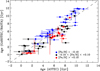 |
Fig. 1. Comparison of stellar ages determined from GARSTEC models with the BASTA programme and ages determined from ASTEC models. The stars have been divided into three metallicity groups as indicated. |
Stellar ages could also have been derived by using spectroscopic gravities instead of luminosities as in Papers I and II, where the available HIPPARCOS parallaxes did not allow a determination of L with sufficient precision. Conversely, we can make a comparison between luminosities and spectroscopic gravities by calculating a “photometric” gravity from the expression
 (3)
(3)
The average difference between the photometric gravity and the spectroscopic gravity is −0.003 dex with an rms deviation of 0.016 dex, which can be explained by the estimated errors of the spectroscopic gravities. As seen from Fig. 2, there is, however, a slight trend of the difference with [Fe/H]:
![Mathematical equation: $$ \begin{aligned} \Delta \mathrm{log}\,g = -0.002 \, (\pm 0.002) + 0.038 \, (\pm 0.013) \cdot \mathrm{[Fe/H]}, \end{aligned} $$](/articles/aa/full_html/2020/08/aa38300-20/aa38300-20-eq4.gif) (4)
(4)
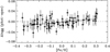 |
Fig. 2. Difference between photometric and spectroscopic gravities as a function of [Fe/H]. The line shows the fit to the data given by Eq. (4). |
as found from a linear regression to the data.
We have first investigated if the trend of Δlog g with [Fe/H] arises because the MARCS models applied for the determination of spectroscopic gravities have a constant helium-to-hydrogen ratio y = NHe/NH = 0.085, whereas the He abundances of the stars depends on [Fe/H] and age. Helium does not contribute to opacity or electrons in solar-type stars but increases the mean molecular weight by a factor of 1+4y and atomic pressure by a factor of 1+y relative to the contributions from hydrogen. As shown by Strömgren et al. (1982, Eq. (12)), a change in the helium-to-hydrogen ratio from y1 to y2 has the same effect on line strengths as a change in gravity from g1 to g2, where
 (5)
(5)
provided that the electron pressure is much smaller than the gas pressure as in the upper layers of the atmospheres of solar-type stars. This equation was used to calculate corrected spectroscopic gravities using y1 = 0.085 and y2 values corresponding to the helium mass fractions in Table 1. The correction goes, however, in the wrong direction and increases the slope of Δlog g versus [Fe/H] by nearly a factor of two. Hence, there must be other systematic errors in the analysis depending on [Fe/H], most likely 3D non-LTE effects on the relative strengths of Fe I and Fe II lines, but deviations from assumptions related to the ASTEC models, such as ΔYi/ΔZi = 1.4 and a constant mixing length parameter could also play a role.
While the trend of Δlog g (phot. − spec.) with [Fe/H] is an interesting problem, it has only a small effect on the derived ages and abundances. If spectroscopic gravities are used in the age determination instead of luminosities, the ages of young, metal-poor stars change by about −0.5 Gyr and ages of young, metal-rich stars by ∼ + 0.5 Gyr. For older more evolved stars, the changes are smaller. Concerning [X/Fe] abundance ratios, the largest effects of using photometric instead of spectroscopic gravities are of the order of ±0.005 dex in the case of C, O, Mg, and Y. These changes are well within the estimated uncertainty of the abundances (see Table 3).
4. Results
In this section, we first show that there are indications of two distinct sequences in the age-metallicity and [X/Fe]-age diagrams. Next, we discuss possible 3D non-LTE effects on the results. Furthermore, we present the [Sr/Mg]- and [Y/Mg]-age relations and discuss their dependence on metallicity with particular emphasis on a puzzling deviation of the visual binary star, ζ Reticuli.
4.1. [Fe/H] and [X/Fe] versus stellar age
The relation between [Fe/H] and stellar age is shown in Fig. 3. As seen, the stars tend to be distributed in two populations: an old sequence (red filled circles) reaching [Fe/H] ∼ + 0.3 at an age of ∼7 Gyr and a younger sequence (blue filled circles) stretching from [Fe/H] ≃ −0.3 at 6 Gyr to [Fe/H] ≃ +0.2 at ∼1 Gyr. Because stars were selected to have 5600 K < Teff < 5950 K, there may be a bias against old metal-rich stars in the upper right corner of the figure and against young metal-poor stars in the lower left corner, but we see no selection effects that could explain the dearth of stars at intermediate ages. Furthermore, although there may be systematic errors affecting the relative ages of stars with different metallicities as discussed in Sect. 3, these errors do not affect the differential ages of stars at a given [Fe/H]. The sample is, however, small, so it could be accidental that there are so few stars between the two populations. Clearly, the possible existence of two distinct sequences in the age-metallicity diagram should be investigated for a larger sample of stars with precise ages and abundances.
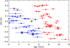 |
Fig. 3. [Fe/H] versus stellar age. The stars have been divided in two groups: an old sequence shown with filled red circles and a younger sequence shown with filled blue circles. Two stars (HD 59711 and HD 183658) having intermediate ages are shown with filled black circles and the Sun with the ⊙ symbol. The components of the visual binary star, ζ Reticuli, are marked with black squares and the Na-rich stars, HD 13724 and HD 189625, with yellow squares. |
Additional evidence of the existence of two distinct chemical evolution sequences comes from the [X/Fe]-age relations shown in Fig. 4. For several of the elements, for example O, Na, Ca, and Ni, there is a discontinuity or bump in [X/Fe] at ∼6 Gyr between the old (red) and young (blue) sequences.
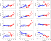 |
Fig. 4. 1D LTE values of [X/Fe] as a function of stellar age for all elements included. Stars are shown with the same symbols as in Fig. 3. |
As seen from Fig. 4, the components of the binary star ζ Reticuli, marked with black squares, show a strong deviation from the mean trends of the s-process elements (Sr and Y) and they also deviate in [C/Fe], [O/Fe], and [Mg/Fe]. This binary star is discussed in Sect. 4.5. Furthermore, two stars, HD 13724 and HD 189625, marked with yellow squares, are enhanced in Na and Ni relative to Fe, whereas they are under-abundant in Sr and Y. Excluding these stars, the scatter in the age trends can be explained by the estimated errors except in the case of the old sequences for Na and Ni. For these two elements, there is, on the other hand, a very good correlation between [Ni/Fe] and [Na/Fe] (see Fig. 5) indicating that the scatter in the age relations are not due to errors in the abundance determinations. A tight correlation between [Ni/Fe] and [Na/Fe] has also been found for metal-poor halo and thick-disk stars (Nissen & Schuster 2010). As suggested by Venn et al. (2004), the correlation can be explained if the production of the most abundant Ni isotope, 58Ni, and 23Na in Type II SNe has the same dependence on neutron excess. If so, the scatter in the [Na/Fe]-age and [Ni/Fe]-age relations may be related to variations in neutron excess of SNe belonging to the old disk population.
4.2. 3D non-LTE effects
Because the stars in this paper were selected to lie on the main sequence and to have effective temperatures in a small range (5600 K < Teff < 5950 K) we expect only small differential 3D non-LTE corrections to the derived abundances at a given [Fe/H]. There may, however, be significant differential corrections when comparing metal-poor with metal-rich stars, which would affect the discontinuities seen in Fig. 4 at an age of ∼6 Gyr.
As reviewed by Barklem (2016), non-LTE corrections based on modern physically-motivated descriptions of cross sections for collisions with hydrogen atoms and electrons are now available for several elements including Mg (Osorio & Barklem 2016) and Al (Nordlander & Lind 2017). These corrections refer, however, to 1D hydrostatic model atmospheres and don’t take into account 3D effects on the spectral lines. In 1D analyses, including that in the present paper, it is assumed that the microturbulence broadening is independent of depth in the stellar atmosphere. In real stellar atmospheres, the hydrodynamical broadening changes with depth and to the extent that lines of different elements are formed at different depths, the derived [X/Fe] values may be in error (Ludwig & Steffen 2016). Obviously, the solution is to carry out a 3D model atmosphere analysis in which line broadening due to atmospheric gas motions follows from the hydrodynamical calculations (Asplund et al. 2000; Allende Prieto et al. 2002).
A non-LTE study of C and O lines based on ab initio calculations of cross sections for collisions with hydrogen atoms tested via solar centre-to-limb observations (Amarsi et al. 2018, 2019a) has recently been carried out by Amarsi et al. (2019b) for a grid of 3D model atmospheres. The results are published as large tables providing 3D non-LTE − 1D LTE corrections as a function of 1D LTE values of Teff, log g, [Fe/H], ξturb, and C or O abundance allowing interpolation to corrections for our set of stars. However, before presenting the results, a special problem with the method used to determine oxygen abundances needs to be addressed.
The O I triplet at 7774 Å is not covered by the HARPS spectra, so we used the weak [O I] line at 6300.3 Å to determine O abundances. As described in Paper I, correction for a blending Ni I line (Allende Prieto et al. 2001) was applied by calculating its EW in the solar and stellar spectra using Ni abundances derived from other Ni I lines and an oscillator strength (log gf = −2.11) measured by Johansson et al. (2003). This procedure could cause systematic errors in the derived O abundances of the more metal-rich stars. The Ni line makes up a larger and larger fraction of the total EW of the 6300.3 Å blend as [Fe/H] is increasing, because [Ni/Fe] is increasing with [Fe/H] (Adibekyan et al. 2012; Bensby et al. 2014) while [O/Fe] is decreasing (Amarsi et al. 2019b). In view of this problem, we have determined oxygen abundances from the O I 7774 Å triplet lines for a subset of stars for which reasonable precise EWs can be measured from ESO/FEROS spectra having R = 48 000 and S/N ∼ 200. For 11 of our stars, EWs of the O I triplet lines can be found in Nissen et al. (2014) and for another 10 stars EWs were measured from FEROS spectra that have become available in the ESO Science Archive after 2014. These EWs were used to derive 1D LTE values of [O/H] and after applying 3D non-LTE corrections from Amarsi et al. (2019b) a comparison was made with 3D non-LTE values of [O/H] based on the [O I] line at 6300.3 Å (see Table 4). As seen from Fig. 6, there is a satisfactory agreement between the two sets of [O/H] values. In particular, there is no trend of the difference as a function of [Fe/H] indicating that the oxygen abundances derived from the forbidden line can be trusted. In this connection, we note that whereas the differential 3D non-LTE corrections are almost negligible for the [O I] line, they range from −0.06 dex to +0.05 dex for the triplet.
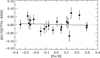 |
Fig. 6. Difference between oxygen abundances derived from the 7774 Å O I triplet and the [O I] 6300 Å line versus [Fe/H] after applying 3D non-LTE corrections from Amarsi et al. (2019b). The full drawn line is a least-squares fit to the data. |
Oxygen abundances derived from the O I 7774 Å triplet and from the [O I] line at 6300 Å.
The differential 3D non-LTE corrections relative to those for the Sun range from −0.015 dex to +0.005 dex for the carbon abundances derived from high-excitation C I lines and from −0.011 dex to +0.003 dex for the oxygen abundances derived from the [O I] line at 6300.3 Å. These small corrections do not lead to any significant change of the 1D LTE trends of [C/Fe] and [O/Fe] with age shown in Fig. 4. The 3D non-LTE effects on the iron abundances may, however, be more important. According to Amarsi et al. (2019b), the [Fe/H] values derived from our Fe II lines are subject to changes ranging from −0.007 dex to +0.025 dex, but 3D non-LTE corrections for the Fe I lines used to determine the atmospheric parameters are not available. Obviously, a 3D non-LTE study of the formation of both Fe I and Fe II lines in the atmospheres of solar-type stars as already carried out for the Sun (Lind et al. 2017) is needed before improved [Fe/H] values can be obtained.
In the case of Ti and Cr, we have determined abundances from respectively three and two lines of the majority species Ti II and Cr II in addition to the abundances given in Table 2 that are based on respectively nine Ti I and seven Cr I lines. As seen from Fig. 7, the abundances from the ionised lines tend to deviate from those of the neutral lines by ∼ + 0.01 dex at the lowest metallicities and ∼ − 0.01 at high [Fe/H]. This suggests that the 1D LTE results shown in Fig. 4 may be affected by differential 3D non-LTE effects at a level of ±0.01 when comparing low- and high-metallicity stars. Again, we need 3D non-LTE studies to improve the accuracy of abundances of these and other elements.
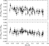 |
Fig. 7. Comparison of Ti and Cr abundances derived from lines belonging to the neutral and ionised species. |
4.3. C/O versus stellar age
The C/O number ratio is important for the structure and composition of planets. The Sun has C/O = 0.56 ± 0.05 (Amarsi et al. 2019a), but if a star and its proto-planetary disk have C/O ≳ 0.8, “Carbon” planets containing large amounts of graphite and carbides instead of Earth-like silicates may be formed (Kuchner & Seager 2005; Bond et al. 2010). Work by Delgado Mena et al. (2010) and Petigura & Marcy (2011) suggested that a significant percentage of high-metallicity solar-type stars have C/O > 0.8, but later studies have not confirmed this (Nissen 2013; Brewer & Fischer 2016; Suárez-Andrés et al. 2018; Amarsi et al. 2019b; Stonkutė et al. 2020). According to these works, there is a rise of C/O with [Fe/H], but none of the stars have C/O significantly larger than 0.8.
As seen from Fig. 8, our 3D non-LTE values of C/O show a rising trend with decreasing age for the old (red) sequence, but all stars have C/O clearly below 0.8. Interestingly, all nine stars with C/O ≃ 0.7 have confirmed planets according to The Extrasolar Planets Encyclopaedia5 (Schneider et al. 2012). These stars have also high metallicities, that is, 0.18 < [Fe/H] < 0.31, so it cannot be decided from the present small sample whether it is the high C/O ratio or the high [Fe/H] (or both) that favour formation of planets.
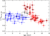 |
Fig. 8. C/O number ratio as a function of stellar age with blue and red filled circles referring to the two sequences Fig. 3. Stars for which one or more planets have been detected are labelled with a black ring. |
4.4. [Y/Mg] and [Sr/Mg] versus age
As mentioned in the Introduction, several studies of solar twins suggest that [Y/Mg] can be used as a sensitive chemical clock to obtain stellar ages (Nissen 2015; Tucci Maia et al. 2016; Spina et al. 2018). Feltzing et al. (2017) found, however, that [Y/Mg] at a given age decreases significantly with decreasing metallicity, but this is less obvious from data presented by Delgado Mena et al. (2019) and Titarenko et al. (2019).
Figure 9 shows a tight [Y/Mg]-age relation for our sample of stars except for a strong deviation of the two components of the visual binary star, ζ Reticuli, and a minor deviation of the two Na-rich stars. Excluding these four stars, an error-weighted maximum likelihood fit gives
![Mathematical equation: $$ \begin{aligned} \mathrm{[Y/Mg]}= 0.179 \, (\pm 0.007) - 0.0383\, (\pm 0.0010) \cdot \mathrm{Age} \,\mathrm{[Gyr]}, \end{aligned} $$](/articles/aa/full_html/2020/08/aa38300-20/aa38300-20-eq6.gif) (6)
(6)
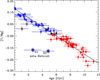 |
Fig. 9. [Y/Mg] versus stellar age with the same symbols as in Fig. 3. The line corresponds to the linear fit given in Eq. (6). |
with a reduced chi-square of 0.82. Within the quoted errors of the zero-point and the slope, this age calibration of [Y/Mg] agrees with the calibration in Paper II for 21 solar twins, whereas Spina et al. (2018) find a somewhat different slope, i.e. −0.045 ± 0.002 for 76 solar twins, which may be due to a different age scale, that is, the use of Yonsei-Yale isochrones (Yi et al. 2001; Kim et al. 2002) instead of the ASTEC isochrones used by us (see discussion in Paper II).
As seen from Fig. 9, there is no indication of a shift in the [Y/Mg]-age relation between the old (red) and the younger (blue) sequence of stars. Furthermore, Fig. 10 shows that the residuals of [Y/Mg] from the age calibration given by Eq. (6) have no significant dependence on metallicity in the −0.3 < [Fe/H] < +0.3 range. In this connection, we note that the shift of [Y/Mg] with [Fe/H] found by Feltzing et al. (2017) occurs for stars with [Fe/H] < −0.3, so there is not necessarily a contradiction between the results of the two investigations.
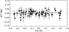 |
Fig. 10. Deviations of [Y/Mg] from Eq. (6) as a function of [Fe/H]. The line shows a linear fit to the data. |
Strontium (Z = 38) belongs to the first peak of s-process elements like yttrium (Z = 39). According to Karakas & Lugaro (2016), the yields of these two elements from Asymptotic Giant Branch (AGB) stars depend in a similar way on stellar mass and metallicity, so one would expect [Sr/Mg] to have about the same dependence on age as [Y/Mg]. As shown in Fig. 11, this is indeed the case; the error-weighted fit to the data gives
![Mathematical equation: $$ \begin{aligned} \mathrm{[Sr/Mg]}= 0.169 \, (\pm 0.007) - 0.0346\, (\pm 0.0010) \cdot \mathrm{Age} \,\mathrm{[Gyr]}, \end{aligned} $$](/articles/aa/full_html/2020/08/aa38300-20/aa38300-20-eq7.gif) (7)
(7)
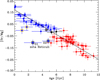 |
Fig. 11. [Sr/Mg] versus stellar age with the same symbols as in Fig. 3. The line shows the linear fit given in Eq. (7). |
when excluding ζ Reticuli and the two Na-rich stars. The scatter around this line is, however, larger than in the case of [Y/Mg] and there is a significant dependence of the residuals on [Fe/H] as seen from Fig. 12. In this connection, we note that the Sr abundances were determined from only one Sr I line (χexc. = 0.0 eV) at 4607.3 Å, which according to Grevesse et al. (2015) is subject to a solar non-LTE correction of +0.15 dex based on calculations by M. Bergemann (priv. comm.). This suggests that there may be significant differential 3D non-LTE corrections depending on [Fe/H]. Yttrium abundances, on the other hand, were determined from three lines. All belong to the Y II majority species and are thus not susceptible to non-LTE overionisation effects. We conclude that until 3D non-LTE calculations become available, [Y/Mg] is to be preferred as a chemical clock.
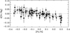 |
Fig. 12. Deviations of [Sr/Mg] from Eq. (7) as a function of [Fe/H]. The line shows the linear fit to the data. |
As recently discussed by Jofré et al. (2020), chemical abundances for 80 solar twins (Spina et al. 2018; Bedell et al. 2018), suggest that a variety of abundance ratios between s-process elements (from Sr to Ce) and lighter elements (from C to Zn) can be used as sensitive chemical clocks. It remains, however, to be investigated to which extent these ratios depend on [Fe/H] at a given age. As an example, our data show that [Y/Al] is more sensitive to age than [Y/Mg], but the residuals in the fit depend significantly on [Fe/H] as in the case of [Sr/Mg].
4.5. The ζ Reticuli binary star
The binary star ζ Ret in the constellation Reticulum is in many ways a most remarkable system. The two components, ζ1 Ret (HD 20766) and ζ2 Ret (HD 20807) have apparent magnitudes of V = 5.51 and V = 5.23, respectively, and with a separation of 5.15 arc minutes they can been seen with the naked eye on a dark sky. According to Gaia DR2 data (Gaia Collaboration 2018), their proper motions, radial velocities, and distances (12.0 pc) agree, suggesting that they have a common origin.
As seen from Fig. 9, both ζ1 and ζ2 Ret fall much below the [Y/Mg]-age relation for the other stars. This is due to an unusually low yttrium abundance compared to other stars with similar ages as shown in Fig. 13, where the spectrum of ζ1 Ret is compared to that of HD 20619. The two stars have about the same values of Teff, log g, and [Fe/H] and the strengths of the Ti I, Fe I, and Ni I lines are nearly the same, whereas the Y II line at 5087.4 Å is weaker in the spectrum of ζ1 Ret resulting in a deficiency, Δ[Y/Fe] = −0.13 dex, of ζ1 Ret relative to HD 20619.
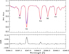 |
Fig. 13. HARPS spectrum of ζ1 Ret (blue line) around the Y II line at 5087.4 Å in comparison with the HARPS spectrum of HD 20619 (red line). The lower panel shows the difference ζ1 Ret – HD 20619. |
In order to illustrate how precisely the ages of ζ1, 2 Ret are determined, Fig. 14 shows their locations in the log (L/L⊙) − Teff diagram in comparison with ASTEC isochrones ranging in age from 0 to 10 Gyr. As the metallicities and [α/Fe] values of the two stars are slightly different, two sets of isochrones corresponding to the heavy element abundances of the stars are shown. Taking into account the estimated uncertainties of Teff and log (L/L⊙) shown with error bars in the figure as well as the uncertainty of the Zs-values of the stars we obtain an age of 2.6 ± 1.3 Gyr for ζ1 Ret and 4.7 ± 0.9 Gyr for ζ2 Ret. Thus, there is a hint of a difference, ΔAge = 2.1 ± 1.6 Gyr, between the ages but this is only significant at the 1.3-sigma level.
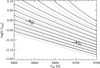 |
Fig. 14. ζ1 and ζ2 Ret in the log (L/Lsun) versus Teff diagram in comparison with ASTEC isochrones ranging in age from 0 to 10 Gyr in steps of 1 Gyr. The full drawn lines refer to isochrones interpolated to the surface heavy element abundance of ζ1, Zs = 0.0122, and the dotted lines to isochrones corresponding to the abundance of ζ2 Ret, Zs = 0.0111. |
Ages of ζ1, 2 Ret may also be estimated from their chromospheric activity. From a detailed study of the Ca II H&K lines in HARPS spectra, Flores et al. (2018) found a period of ∼10 yr in the activity of ζ2 Ret with approximately the same level of Ca II H&K core emission as the Sun. ζ1 Ret is much more active as can be seen from Fig. 15. No activity cycle was detected by Flores et al. (2018) but the emission in the cores of the Ca II H&K lines varies over the 3.3 yr period covered by the HARPS spectra. The average chromospheric Ca II H&K emission index ( ) determined for the two stars (see Table 2 in Flores et al. 2018) is log
  for ζ1 Ret and log
  for ζ2 Ret. From these values and the open cluster age calibration of log
  by Mamajek & Hillenbrand (2008), which has a scatter of ±0.07 dex in log
  , we estimate ages of 1.8 ± 0.8 Gyr for ζ1 Ret and 4.10 ± 1.1 for ζ2 Ret in agreement with the isochrone ages within the estimated errors.
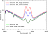 |
Fig. 15. HARPS spectra of ζ1 and ζ2 Ret near the centre of the Ca II K line in comparison with the solar flux HARPS spectrum observed as reflected light from Vesta in 2011. The flux is given relative to the continuum flux in the region of the Ca II H&K lines. |
The chemical evolution ages of the ζ Ret stars are significantly higher than their isochrone and activity ages. From the [Y/Mg] values we derive 9.1 ± 0.5 Gyr for ζ1 Ret and 9.4 ± 0.5 Gyr for ζ2 Ret based on the calibration in Eq. (6). A similar problem was presented by Rocha-Pinto et al. (2002), who noted that ζ1 Ret is chromospherically young but kinematically old. Its Galactic velocity components with respect to the Local Standard of Rest (LSR) are (U, V, W) = (−63, −34, +23) km s−1, indicating that it belongs to the old disk. As an explanation, Rocha-Pinto et al. (2002) suggested that such stars are blue stragglers formed from the coalescence of short-period binaries with low-mass components. This scenario also explains the difference between isochrone age and chemical evolution age of ζ1, 2 Ret. It may even explain the possible difference in isochrone age between ζ1 and ζ2 Ret, because the coalescence could happen at different times. Furthermore, the scenario can explain that both stars are severely depleted in lithium and beryllium (Santos et al. 2004) relative to stars with similar mass, age, and metallicity, because Li and Be destruction would take place in the deep convection zones of the low-mass stars.
It is more difficult to explain that ζ1 and ζ2 Ret do not have the same chemical composition. Saffe et al. (2016) used HARPS spectra with S/N ∼ 300 obtained on a single night to show that abundances of refractory elements in ζ1 Ret are enhanced relative to the abundances in ζ2 Ret. Furthermore, they found that the abundance difference increases as a function of elemental condensation temperature (Tc) (Lodders 2003) with a slope of 3.85 (±1.02)⋅10−5 dex K−1. This was confirmed by Adibekyan et al. (2016) based on combined HARPS spectra of ζ1 and ζ2 Ret having S/Ns as high as 1300 and 3000, respectively. As seen from Fig. 16, our abundances also show a difference between ζ1 and ζ2 Ret correlated with elemental condensation temperature; a weighted least squares fit leads to the relation
![Mathematical equation: $$ \begin{aligned} \Delta \mathrm{[X/H]}= 0.002 (\pm 0.015) + 3.15 \, (\pm 1.13) 10^{-5} \cdot T_{\rm c} \, \mathrm{dex\,K}^{-1}, \end{aligned} $$](/articles/aa/full_html/2020/08/aa38300-20/aa38300-20-eq13.gif) (8)
(8)
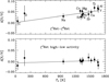 |
Fig. 16. Abundance difference between ζ1 and ζ2 Ret as a function of elemental condensation temperature (upper panel) compared to the difference in abundances derived for ζ1 Ret in respectively the high and low activity phases shown in Fig. 15 (lower panel). |
in agreement with the results of Saffe et al. (2016) and Adibekyan et al. (2016).
Yana Galarza et al. (2019) have shown that some of the stronger Fe I and Fe II lines in HARPS spectra of the young active solar twin HD 59967 vary significantly in strength along its activity cycle of ∼6 yr and that the derived atmospheric parameters change correspondingly with an amplitude of ∼30 K in Teff and 0.015 dex in [Fe/H]. A similar result was obtained by Spina et al. (2020) for a large sample of active solar-type stars. This raises the question if our derived abundances for ζ1 Ret also depend on its level of activity. We have therefore analysed two sets of HARPS spectra, each with S/N ∼ 800, obtained during respectively the high and low activity phases (see Fig. 15). The derived Teff’s differ by 10 K only and as shown in Fig. 16 (lower panel), there is no significant difference between the abundances obtained during the two activity phases. This supports that our derived abundances are not significantly affected by magnetic activity and that the abundance enhancement of ζ1 Ret relative to ζ2 Ret cannot be explained by the difference in activity. We note in this connection that ζ1 Ret is not as active as HD 59967 and that we are using weaker Fe lines, less sensitive to magnetic fields, than those used by Yana Galarza et al. (2019) and Spina et al. (2020) to determine atmospheric parameters and abundances.
As recently listed by Ramírez et al. (2019, Table 6), there is now ten known twin-star comoving pairs with a significant difference in the abundance of refractory elements. In some cases the difference reaches ∼0.2 dex (Oh et al. 2018; Ramírez et al. 2019; Nagar et al. 2020) and is correlated with elemental condensation temperature. Possible explanations of the abundance differences include sequestration of refractory elements in planets (Meléndez et al. 2009; Chambers 2010), engulfment of planets (Meléndez et al. 2017; Tucci Maia et al. 2019), and dust-gas separation in star-forming gas clouds or circumstellar disks (Gaidos 2015; Gustafsson 2018a,b). In this connection, we note that no planets have been detected around the ζ Ret stars, but infrared observations with the Spitzer and Herschel telescopes suggested the existence of a debris disk around ζ2 Ret (Trilling et al. 2008; Eiroa et al. 2010). ALMA/Atacama Compact Array (sub)mm observations carried out 8 years after the Herschel observations show, however, that the disk does not share the large proper motion of ζ2 Ret and is probably a background source (Faramaz et al. 2018). Therefore, it remains unclear how the abundance difference between ζ1 and ζ2 Ret should be explained.
5. Discussion
When discussing explanations of the two sequences for [Fe/H] and [X/Fe] as a function of stellar age, it should be remembered that the stars have been selected to have an approximately uniform distribution in [Fe/H] from ∼ − 0.3 dex to ∼ + 0.3 dex. For this range, the separation in low- and high-alpha stars is not as clear as in the range −0.6 ≲ [Fe/H] ≲ −0.3 (e.g. Adibekyan et al. 2012; Bensby et al. 2014; Fuhrmann et al. 2017). Instead, we have found indication of a dichotomy of the distribution of stars in the [Fe/H]-age diagram.
One may wonder why the two age sequences have not been seen in previous studies of the age-metallicity relation for solar-type stars, but for typical age precisions of 2–4 Gyr, the dearth of stars at intermediate ages seen in Fig. 3 tends to be washed out. A higher age precision was claimed by Haywood et al. (2013), who in a study of the Adibekyan et al. (2012) sample estimated errors of 0.8–1.5 Gyr for isochrone ages of somewhat evolved main-sequence stars. Interestingly, they found a tight age-metallicity relation for high-alpha (thick disk) stars similar to the old sequence in our Fig. 3, but there is no split into two distinct age sequences in their age-metallicity diagram (see Fig. 9 in Haywood et al. 2013). The reason may be that Haywood et al. include stars from a broad range in effective temperature, 5000 K ≲Teff ≲ 6400 K, which means that systematic errors in the isochrones as a function of stellar mass add to the statistical errors. Our study is limited to stars with 5600 K < Teff < 5950 K allowing us to make a differential determination of isochrone ages relative to the well known age of the Sun and therefore obtain ages with a precision of 0.5–1.3 Gyr for stars with similar [Fe/H]. Furthermore, the precision of our derived effective temperatures is of the order of 10 K compared to 25-70 K for the stars in Adibekyan et al. (2012), which is important for the derivation of precise ages especially for stars near the ZAMS.
Concerning investigations based on asteroseismic ages, we note that the analysis by Silva Aguirre et al. (2018) of ∼1200 red giants with precise abundances from APOGEE (the so-called APOKASC sample) does not show any split of the age-metallicity relation into two sequences. The seismic ages have, however, errors of about 20–40% depending on whether a star belongs to the red giant branch or the clump phase. This means that stars with ages in the range 5–10 Gyr have typical age uncertainties of 1.5–3 Gyr, so again one cannot expect to detect the dearth of stars with intermediate ages seen in Fig. 3. The smaller sample of solar-type dwarfs for which high-precision individual oscillation frequencies are available from Kepler short-cadence observations (Huber et al. 2013; Lund et al. 2017) is more interesting in this connection. Silva Aguirre et al. (2015) analysed 33 such stars with planets and Silva Aguirre et al. (2017) 66 stars without known planets, the so-called LEGACY sample. They obtained age uncertainties of 10–15% from the asteroseismic data. Metallicities are, on the other hand, not very precise for many of these stars; ten stars have [Fe/H] determined from high S/N HARPS-N spectra with a precision of ∼0.02 dex (Nissen et al. 2017), but for the rest [Fe/H] was derived from low S/N spectra with a precision of ∼0.10 dex. Nevertheless, the age-metallicity diagram for the Kepler dwarfs (see Fig. 17) gives support to the existence of an old and a young sequence with a deficit of stars in between, although details such as the [Fe/H]-age slope for the two populations and the width of their separation are somewhat different from the corresponding features in the ASTEC age-metallicity diagram. The deficit of stars at intermediate ages was in fact noted by Silva Aguirre et al. (2015) but was ascribed to a selection effect, namely that detection of oscillations by Kepler is favoured for the brighter stars, either young F-type or old evolved G-type stars. After addition of the LEGACY sample, Fig. 17 includes, however, ten unevolved (4.27 < log g < 4.50), cool (5500 K < Teff < 6150 K stars with ages corresponding to those of the young sequence. Stars with intermediate ages are more evolved and have larger oscillation amplitudes. Therefore, it is unlikely that the deficit of stars at intermediate ages is a selection effect. The absence of stars younger than ∼1.5 Gyr is on the other hand a selection bias; Such stars lie either close to the ZAMS and have low oscillation amplitudes or are warmer than Teff ∼ 6600 K, the temperature limit of the Kepler dwarf sample.
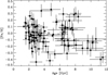 |
Fig. 17. Age-metallicity diagram for dwarf stars with ages determined from Kepler short-cadence observations of individual oscillation frequencies by Silva Aguirre et al. (2015, 2017). |
As a possible explanation of the two age sequences in Fig. 3, we have considered the “two-infall” chemical evolution model of Chiappini et al. (1997) as revised by Grisoni et al. (2017). This model assumes two main episodes of infalling gas onto the Galactic disk corresponding to the formation of respectively the thick and the thin disk. Spitoni et al. (2019, 2020) have recently compared the predictions of this model with APOGEE chemical abundances and seismic ages of K giants in the APOKASC sample (Silva Aguirre et al. 2018) and have shown that a significant delay of 4.5–5.5 Gyr between the two episodes of gas accretion is needed to explain the data. The corresponding star formation rate has a minimum at an age of ∼8 Gyr. A similar quenching of star formation around an age of 8 Gyr was derived by Snaith et al. (2015) from the Adibekyan et al. (2012) abundances and the Haywood et al. (2013) isochrone ages of solar-type stars. There is also indications of a double-peaked star formation history, although with a minimum around 6 Gyr, from Gaia colour-magnitude diagrams (Mor et al. 2019). Furthermore, several models of galaxy formation predict a quenching of star formation at ages between 6 and 9 Gyr. Noguchi (2018) suggests that high-alpha stars form during an initial phase of accretion of cold primordial gas followed by a hiatus until the shock-heated gas has cooled due to radiation and a new accretion begins leading to the formation of low-alpha disk stars. Cosmological hydrodynamical simulations also point to the formation of bimodal disks (e.g. Grand et al. 2018) possibly triggered by a gas-rich merging satellite (Buck 2020).
Using the Markov Chain Monte Carlo (MCMC) method described by Spitoni et al. (2020), we have made a preliminary investigation of how well the two-infall model fits the observed [Fe/H]-, [O/Fe]-, and [Mg/Fe]-age relations. The solar neighbourhood is assumed to have a metallicity of [Fe/H] = −1 at an age of 12 Gyr at which time the first exponentially decaying infall of primordial gas begins followed by a delayed second infall of primordial gas. The main parameters of the model are the timescales of the infalling gas, τ1 and τ2, and the delay time, Tdelay. More details about the model may be found in Spitoni et al. (2019, 2020) including assumptions about the star formation efficiency, stellar yields, the Initial Mass Function (IMF), and the delay of Type Ia SNe relative to Type II SNe.
The two-infall model describes the evolution of chemical abundances in interstellar gas and should therefore be compared to the initial composition of stars. Hence, the present observed surface abundances should be corrected for diffusion before comparison with the model predictions. According to the ASTEC models, the difference [Fe/H]initial − [Fe/H] is 0.054 dex for the Sun, rises to about 0.10 dex for ∼10 Gyr old stars, and is near zero for the youngest stars in our sample. Therefore, the age slope of [Fe/H]initial is somewhat different from the slope of [Fe/H]. This has been taken into account in the MCMC fitting of the two-infall model to our data. The diffusion effect on [O/Fe] and [Mg/Fe] may, on the other hand, be neglected, because the abundances of these elements are affected in approximately the same way (see Turcotte et al. 1998, Fig. 14).
Figure 18 shows the MCMC fitting of the two-infall model to our data. The resulting parameter values are τ1 = 0.38 ± 0.04 Gyr, τ2 = 3.2 ± 0.4 Gyr, and Tdelay = 3.52 ± 0.05 Gyr. The delay time is similar to the value obtained from the MCMC fitting of the APOKASC data by Spitoni et al. (2020) (Tdelay = 4.62 ± 0.12 Gyr), but the infall timescales are shorter than the values obtained for the APOKASC sample (τ1 = 1.26 ± 0.10 Gyr and τ2 = 11.3 ± 0.9 Gyr).
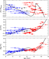 |
Fig. 18. Comparison of the [Fe/H]initial-, [O/Fe]-, and [Mg/Fe]-age relations with predictions from the two-infall chemical evolution model. |
As seen from Fig. 18, the two-infall model explains the main features of the abundance-age relations, but there are problems with the details. In the upper panel, the model predicts too high ages for the old sequence. This part of the fit is improved if the model begins with [Fe/H] = −1 at an age of 11 Gyr instead of 12 Gyr, but then the fit to the steep decline of [O/Fe] and [Mg/Fe] at high ages is less satisfactory. Furthermore, the model does not reach the group of 12 metal-rich stars on the old sequence having [O/Fe] ∼ −0.1 and a too large bump in [Mg/Fe] is predicted at ages between 6 and 8 Gyr. Finally the model predicts a too steep decline of [Mg/Fe] at ages below 5 Gyr.
It is beyond the scope of this paper to investigate if the fitting of the two-infall model to the data can be improved by varying the yields or by changing assumptions about the star-formation history, the IMF, the time-scale of Type Ia SNe, and the composition of the infalling gas. A comparison with the age trends of other element ratios, such as [Na/Fe], [Ni/Fe], and [Y/Mg], is also postponed. Instead, we briefly discuss if the alternative scenario of forming the thick and the thin disks proposed by Haywood et al. (2019) can explain the two sequences in the age-metallicity diagram and the corresponding age trends of element ratios.
According to Haywood et al. (2019), high-alpha stars started to form in a turbulent gaseous thick disk with a chemical evolution described by the closed-box model. After 3–4 Gyr, the gas had been enriched to solar metallicity but then experienced a quenching of star formation possibly caused by formation of a central bar (Haywood et al. 2018). At the same time, accretion of metal-poor gas mixed with solar-metallicity gas from the thick disk began in the outer parts of the disk leading to the formation of the thin disk. In the solar neighbourhood, this caused a decrease of metallicity to [Fe/H] ∼ −0.2, but farther out in the disk a lower metallicity was reached because of a higher portion of metal-poor gas. In this way, a radial metallicity gradient in the thin disk was created. After the quenching period, the chemical evolution continued leading to the formation of metal-rich stars ([Fe/H] ∼ +0.3) in the inner disk (galactocentric distances RG < 7 kpc) and a gradual increase of [Fe/H] with age in the outer disk (see Fig. 6 in Haywood et al. 2019, for a sketch of the resulting age trends of [Fe/H] and [α/Fe]). The trends are similar to the predictions of the two-infall model shown in Fig. 18, but with a turnover in [Fe/H] at solar metallicity instead of [Fe/H] = +0.3 probably leading to a smaller bump in [Mg/Fe] at ages between 6 and 8 Gyr in better agreement with the data. The metal-rich group of stars with low values of [O/Fe] could then be interpreted as formed at the end of the inner disk evolution. It remains, however, to be seen how well a detailed chemical evolution model for this scenario can explain the data in Fig. 18.
In connection with the Haywood et al. (2019) scenario, the kinematics of our stars is of interest. Galactic velocity components, U, V, W, and peri- and apo-galactic orbital distances from the Galactic centre, Rperi and Rapo, were adopted from Holmberg et al. (2009), who used Tycho-2 proper motions (Høg et al. 2000), HIPPARCOS distances (van Leeuwen 2007), and radial velocities from the Geneva-Copenhagen survey (Nordström et al. 2004) in their calculations. As seen from the resulting Toomre diagram in Fig. 19, the old (red) population has a larger velocity dispersion and a larger rotational lag with respect to the LSR than the young (blue) population. This difference in kinematics is also evident from the mean galactocentric distances in the stellar orbits Rm = (Rperi + Rapo)/2. The old population has an average ⟨Rm⟩ = 7.34 kpc with an rms dispersion of σ = 0.71 kpc. The younger population has ⟨Rm⟩ = 7.82 kpc and σ = 0.44 kpc. Assuming that Rm is a measure of the galactocentric distance of the stellar birthplace (e.g. Edvardsson et al. 1993), these values support that the old stars were formed inside the mean galactocentric distance for the formation of the younger population, but the difference in ⟨Rm⟩ is small, so the kinematics does not provide much evidence of the Haywood et al. (2019) disk formation scenario. If, on the other hand, the orbital angular momenta of the old stars have been changed, we cannot use Rm as a proxy of stellar birthplace and therefore the stars may have been formed farther away.
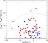 |
Fig. 19. Toomre diagram for stars on the two age sequences in Fig. 3. Stars on the old age sequence are shown with filled red circles and those on the younger age sequence with filled blue circles. The dotted lines correspond to respectively Vtotal = 50 km s−1 and Vtotal = 100 km s−1. The uncertainty of the velocity components is about 1.5 km s−1, corresponding to the size of the circles. |
6. Summary and conclusions
High-precision chemical abundances have been determined from HARPS spectra of 72 nearby solar-type stars and precise ages were derived by comparing spectroscopic effective temperatures and luminosities based on Gaia DR2 distances to ASTEC isochrones. These data suggest that there are two distinct sequences in the age-metallicity diagram (Fig. 3). A similar distribution is seen in the age-metallicity diagram of dwarf stars for which precise asteroseismic ages have been determined from Kepler satellite observations of oscillation frequencies (Fig. 17). The two sequences can also be seen as distinct [X/Fe]-age trends for several elements, most notable O, Na, Ca, and Ni (Fig. 4).
Previous studies of the age-metallicity relation for stars in the solar neighbourhood have not revealed any bimodal distribution. This can be ascribed to typical age uncertainties of 2–4 Gyr, which blurs the age gap between the two sequences leading to an apparently flat distribution of [Fe/H] as a function of age. The corresponding large scatter in [Fe/H] at a given age has been explained as due to migration of stars over several kpc in a Galactic disk with a radial metallicity gradient and this has been the most important argument for the existence of ‘churning’ (changes of orbital angular momentum) in addition to ‘blurring’ (increase in epicycle amplitude in time). With two distinct sequences in the age-metallicity diagram, the scatter in [Fe/H] at a given age for each sequence is decreased and it is a question if ‘churning’ is needed to explain the data.
The elemental abundances provided in this paper have been derived by analysing HARPS spectra with 1D model atmospheres under the LTE assumption. As discussed in Sect. 4, a 3D non-LTE analysis may lead to changes of the derived abundances and atmospheric parameters and therefore also the derived ages, although the cases of C and O, for which 3D non-LTE corrections are available, suggest that differential corrections are small for the lines and stars considered in the present work. Still, it would be important to extend 3D non-LTE calculations to other elements than C and O, in particular to the Fe I lines used to derive Teff and log g. 3D non-LTE corrections may also affect the derived jumps in some abundance ratios between metal-rich stars on the old age sequence and metal-poor stars on the younger sequence for ages at 6–7 Gyr, and therefore be important when testing chemical evolution models.
As discussed in Sect. 5, the two-infall chemical evolution model (Chiappini et al. 1997; Spitoni et al. 2019) provides an overall satisfactory fit to the distribution of stars in the [Fe/H]initial-, [O/Fe]-, and [Mg/Fe]-age diagrams, but some details such as the existence of a group of metal-rich stars with [O/Fe] ∼ −0.10 cannot be explained. It also remains to be investigated if other abundance trends, in particular [Y/Mg] versus age, can be explained. [Y/Mg] shows a remarkable steep and tight trend as function of age (except for a puzzling deviation of the visual binary star ζ Ret) with no offset between the two age sequences and with negligible dependence on metallicity in the range −0.3 < [Fe/H] < +0.3.
As an alternative to the two-infall model, it should be investigated if the scenario proposed by Haywood et al. (2019), in which the inner thick disk evolves according to the closed box model and the outer thin disk forms from infalling metal-poor gas, can explain the data. Given that the Sun is situated at the transition between the two regions, the solar neighbourhood may consist of a mixture of stars having experienced two different chemical evolution tracks.
Given the relative small sample of stars studied, it would be important to investigate if larger samples with high precision abundances and ages confirm the split of the age-metallicity diagram into two age sequences. It requires, however, spectra of a similar high quality as the HARPS spectra applied in this paper to determine abundances and isochrone ages with sufficient precision to detect the gap between the two age sequences. Another interesting possibility is to expand the sample of solar-type stars with seismic ages derived from individual oscillation frequencies using for example TESS satellite data.
For two elements, A and B, having number densities NA and NB, [A/B] ≡ log(NA/NB)star − log(NA/NB)⊙.
α denotes the abundance of alpha-capture elements. In this paper, α is calculated as the mean value of the abundances of Mg, Si, and Ti.
The excluded lines are: Mg I 4730.04 Å, Si I 5793.08 Å, Ti I 5739.48 and 5866.46 Å, Ti II 5381.03 Å, Cr I 5247.57, 5296.70, and 5348.33 Å, Fe I 5466.99 and 6157.73 Å, Fe II 6416.93 Å, Ni I 6108.12 and 6643.64 Å.
Acknowledgments
We thank Anish Amarsi and Bengt Gustafsson for helpful comments on a first version of the manuscript and the referee for a very constructive report on the paper. Funding for the Stellar Astrophysics Centre is provided by The Danish National Research Foundation (Grant agreement no.: DNRF106). V. S. A. acknowledges support from the Independent Research Fund Denmark (Research grant 7027-00096B). V. S. A. and J. R. M. acknowledge support from the Carlsberg foundation (grant agreement CF19-0649). This research has made use of the SIMBAD database, operated at CDS, Strasbourg, France, as well as data from the European Space Agency (ESA) mission Gaia (https://www.cosmos.esa.int/gaia), processed by the Gaia Data Processing and Analysis Consortium (DPAC, https://www.cosmos.esa.int/web/gaia/dpac/consortium). Funding for the DPAC has been provided by national institutions, in particular the institutions participating in the Gaia Multilateral Agreement. Based on observations collected at the European Southern Observatory under ESO HARPS programmes 060.A-9036, 072.C-0488, 072.C-0513, 073.D-0578, 074.C-0012, 076.C-0878, 077.C-0530, 078.C-0833, 078.C-0044, 079.C-0681, 085.C-0019, 089.C-0732, 091.C-0936, 092.C-0721, 093.C-0409, 093.C-0919, 094.C-0901, 097,C-0571, 100.D-0444, 101.C-0275, 102.C-0584, 183.C-0972, 183.D-0729, 188.C-0265, 192.C-0224, 192.C-0852, 196.C-1006, 198.C-0836, and ESO FEROS programmes 092.A-9002, 095.A-9029, 099.A-9022, 100.A-9022.
References
- Adibekyan, V. Z., Sousa, S. G., Santos, N. C., et al. 2012, A&A, 545, A32 [NASA ADS] [CrossRef] [EDP Sciences] [Google Scholar]
- Adibekyan, V., Delgado-Mena, E., Figueira, P., et al. 2016, A&A, 591, A34 [NASA ADS] [CrossRef] [EDP Sciences] [Google Scholar]
- Allende Prieto, C., Lambert, D. L., & Asplund, M. 2001, ApJ, 556, L63 [NASA ADS] [CrossRef] [Google Scholar]
- Allende Prieto, C., Asplund, M., García López, R. J., & Lambert, D. L. 2002, ApJ, 567, 544 [NASA ADS] [CrossRef] [Google Scholar]
- Amarsi, A. M., Barklem, P. S., Asplund, M., Collet, R., & Zatsarinny, O. 2018, A&A, 616, A89 [NASA ADS] [CrossRef] [EDP Sciences] [Google Scholar]
- Amarsi, A. M., Barklem, P. S., Collet, R., Grevesse, N., & Asplund, M. 2019a, A&A, 624, A111 [NASA ADS] [CrossRef] [EDP Sciences] [Google Scholar]
- Amarsi, A. M., Nissen, P. E., & Skúladóttir, Á. 2019b, A&A, 630, A104 [NASA ADS] [CrossRef] [EDP Sciences] [Google Scholar]
- Anders, F., Chiappini, C., Minchev, I., et al. 2017, A&A, 600, A70 [NASA ADS] [CrossRef] [EDP Sciences] [Google Scholar]
- Asplund, M., Nordlund, Å., Trampedach, R., Allende Prieto, C., & Stein, R. F. 2000, A&A, 359, 729 [Google Scholar]
- Asplund, M., Grevesse, N., Sauval, A. J., & Scott, P. 2009, ARA&A, 47, 481 [NASA ADS] [CrossRef] [Google Scholar]
- Barklem, P. S. 2016, A&ARv, 24, 9 [NASA ADS] [CrossRef] [Google Scholar]
- Basu, S., & Antia, H. M. 2004, ApJ, 606, L85 [NASA ADS] [CrossRef] [Google Scholar]
- Bedell, M., Bean, J. L., Meléndez, J., et al. 2018, ApJ, 865, 68 [NASA ADS] [CrossRef] [Google Scholar]
- Bensby, T., Feltzing, S., Lundström, I., & Ilyin, I. 2005, A&A, 433, 185 [NASA ADS] [CrossRef] [EDP Sciences] [Google Scholar]
- Bensby, T., Feltzing, S., & Oey, M. S. 2014, A&A, 562, A71 [NASA ADS] [CrossRef] [EDP Sciences] [Google Scholar]
- Bond, J. C., O’Brien, D. P., & Lauretta, D. S. 2010, ApJ, 715, 1050 [NASA ADS] [CrossRef] [Google Scholar]
- Brewer, J. M., & Fischer, D. A. 2016, ApJ, 831, 20 [NASA ADS] [CrossRef] [Google Scholar]
- Buck, T. 2020, MNRAS, 491, 5435 [NASA ADS] [CrossRef] [Google Scholar]
- Buder, S., Lind, K., Ness, M. K., et al. 2019, A&A, 624, A19 [NASA ADS] [CrossRef] [EDP Sciences] [Google Scholar]
- Casagrande, L., Ramírez, I., Meléndez, J., Bessell, M., & Asplund, M. 2010, A&A, 512, A54 [NASA ADS] [CrossRef] [EDP Sciences] [Google Scholar]
- Casagrande, L., Schönrich, R., Asplund, M., et al. 2011, A&A, 530, A138 [NASA ADS] [CrossRef] [EDP Sciences] [Google Scholar]
- Chambers, J. E. 2010, ApJ, 724, 92 [NASA ADS] [CrossRef] [Google Scholar]
- Chiappini, C., Matteucci, F., & Gratton, R. 1997, ApJ, 477, 765 [Google Scholar]
- Christensen-Dalsgaard, J. 2008, Ap&SS, 316, 13 [NASA ADS] [CrossRef] [Google Scholar]
- Christensen-Dalsgaard, J., & Pérez Hernández, F. 1991, in Challenges to Theories of the Structure of Moderate-Mass Stars, eds. D. Gough, & J. Toomre (Berlin Springer Verlag), Lect. Notes Phys., 388, 43 [CrossRef] [Google Scholar]
- Cutri, R. M., Skrutskie, M. F., van Dyk, S., et al. 2003, VizieR Online Data Catalog, II/246 [Google Scholar]
- da Silva, R., Porto de Mello, G. F., Milone, A. C., et al. 2012, A&A, 542, A84 [NASA ADS] [CrossRef] [EDP Sciences] [Google Scholar]
- Delgado Mena, E., Israelian, G., González Hernández, J. I., et al. 2010, ApJ, 725, 2349 [NASA ADS] [CrossRef] [Google Scholar]
- Delgado Mena, E., Moya, A., Adibekyan, V., et al. 2019, A&A, 624, A78 [NASA ADS] [CrossRef] [EDP Sciences] [Google Scholar]
- Edvardsson, B., Andersen, J., Gustafsson, B., et al. 1993, A&A, 275, 101 [NASA ADS] [Google Scholar]
- Eiroa, C., Fedele, D., Maldonado, J., et al. 2010, A&A, 518, L131 [NASA ADS] [CrossRef] [EDP Sciences] [Google Scholar]
- Epstein, C. R., Johnson, J. A., Dong, S., et al. 2010, ApJ, 709, 447 [NASA ADS] [CrossRef] [Google Scholar]
- Faramaz, V., Bryden, G., Stapelfeldt, K. R., et al. 2018, MNRAS, 481, 44 [CrossRef] [Google Scholar]
- Feltzing, S., Holmberg, J., & Hurley, J. R. 2001, A&A, 377, 911 [NASA ADS] [CrossRef] [EDP Sciences] [Google Scholar]
- Feltzing, S., Howes, L. M., McMillan, P. J., & Stonkutė, E. 2017, MNRAS, 465, L109 [NASA ADS] [CrossRef] [Google Scholar]
- Feuillet, D. K., Frankel, N., Lind, K., et al. 2019, MNRAS, 489, 1742 [NASA ADS] [CrossRef] [Google Scholar]
- Flores, M., Saffe, C., Buccino, A., et al. 2018, MNRAS, 476, 2751 [NASA ADS] [CrossRef] [Google Scholar]
- Frankel, N., Rix, H.-W., Ting, Y.-S., Ness, M., & Hogg, D. W. 2018, ApJ, 865, 96 [NASA ADS] [CrossRef] [Google Scholar]
- Fuhrmann, K. 1998, A&A, 338, 161 [NASA ADS] [Google Scholar]
- Fuhrmann, K., Chini, R., Kaderhandt, L., & Chen, Z. 2017, MNRAS, 464, 2610 [Google Scholar]
- Gaia Collaboration (Brown, A. G. A., et al.) 2018, A&A, 616, A1 [NASA ADS] [CrossRef] [EDP Sciences] [Google Scholar]
- Gaidos, E. 2015, ApJ, 804, 40 [NASA ADS] [CrossRef] [Google Scholar]
- Grand, R. J. J., Bustamante, S., Gómez, F. A., et al. 2018, MNRAS, 474, 3629 [NASA ADS] [CrossRef] [Google Scholar]
- Gratton, R. G., Carretta, E., Matteucci, F., & Sneden, C. 2000, A&A, 358, 671 [NASA ADS] [Google Scholar]
- Gray, D. F. 1992, in The Observation and Analysis of Stellar Photospheres, Camb. Astrophys. Ser. (Cambridge: Cambridge Univ. Press) 20 [Google Scholar]
- Grevesse, N., Noels, A., & Sauval, A. J. 1996, in Cosmic Abundances, eds. S. S. Holt, & G. Sonneborn, ASP Conf. Ser., 99, 117 [Google Scholar]
- Grevesse, N., Scott, P., Asplund, M., & Sauval, A. J. 2015, A&A, 573, A27 [NASA ADS] [CrossRef] [EDP Sciences] [Google Scholar]
- Grisoni, V., Spitoni, E., Matteucci, F., et al. 2017, MNRAS, 472, 3637 [Google Scholar]
- Gustafsson, B. 2018a, A&A, 616, A91 [NASA ADS] [CrossRef] [EDP Sciences] [Google Scholar]
- Gustafsson, B. 2018b, A&A, 620, A53 [CrossRef] [EDP Sciences] [Google Scholar]
- Gustafsson, B., Edvardsson, B., Eriksson, K., et al. 2008, A&A, 486, 951 [NASA ADS] [CrossRef] [EDP Sciences] [Google Scholar]
- Hayden, M. R., Bovy, J., Holtzman, J. A., et al. 2015, ApJ, 808, 132 [Google Scholar]
- Haywood, M., Di Matteo, P., Lehnert, M. D., Katz, D., & Gómez, A. 2013, A&A, 560, A109 [NASA ADS] [CrossRef] [EDP Sciences] [Google Scholar]
- Haywood, M., Di Matteo, P., Lehnert, M., et al. 2018, A&A, 618, A78 [NASA ADS] [CrossRef] [EDP Sciences] [Google Scholar]
- Haywood, M., Snaith, O., Lehnert, M. D., Di Matteo, P., & Khoperskov, S. 2019, A&A, 625, A105 [CrossRef] [EDP Sciences] [Google Scholar]
- Høg, E., Fabricius, C., Makarov, V. V., et al. 2000, A&A, 355, L27 [Google Scholar]
- Holmberg, J., Nordström, B., & Andersen, J. 2009, A&A, 501, 941 [NASA ADS] [CrossRef] [EDP Sciences] [Google Scholar]
- Huber, D., Chaplin, W. J., Christensen-Dalsgaard, J., et al. 2013, ApJ, 767, 127 [NASA ADS] [CrossRef] [Google Scholar]
- Jofré, P., Jackson, H., & Tucci Maia, M. 2020, A&A, 633, L9 [CrossRef] [EDP Sciences] [Google Scholar]
- Johansson, S., Litzén, U., Lundberg, H., & Zhang, Z. 2003, ApJ, 584, L107 [NASA ADS] [CrossRef] [Google Scholar]
- Karakas, A. I., & Lugaro, M. 2016, ApJ, 825, 26 [NASA ADS] [CrossRef] [Google Scholar]
- Kim, Y.-C., Demarque, P., Yi, S. K., & Alexander, D. R. 2002, ApJS, 143, 499 [NASA ADS] [CrossRef] [Google Scholar]
- Kuchner, M. J., & Seager, S. 2005, ArXiv e-prints [arXiv: astro-ph/0504214] [Google Scholar]
- Lind, K., Amarsi, A. M., Asplund, M., et al. 2017, MNRAS, 468, 4311 [NASA ADS] [CrossRef] [EDP Sciences] [Google Scholar]
- Lindegren, L., Hernández, J., Bombrun, A., et al. 2018, A&A, 616, A2 [NASA ADS] [CrossRef] [EDP Sciences] [Google Scholar]
- Lodders, K. 2003, ApJ, 591, 1220 [NASA ADS] [CrossRef] [Google Scholar]
- Ludwig, H. G., & Steffen, M. 2016, Astron. Nachr., 337, 844 [NASA ADS] [CrossRef] [Google Scholar]
- Lund, M. N., Silva Aguirre, V., Davies, G. R., et al. 2017, ApJ, 835, 172 [CrossRef] [Google Scholar]
- Mamajek, E. E., & Hillenbrand, L. A. 2008, ApJ, 687, 1264 [NASA ADS] [CrossRef] [Google Scholar]
- Mayor, M., Pepe, F., Queloz, D., et al. 2003, Messenger, 114, 20 [Google Scholar]
- Meléndez, J., Asplund, M., Gustafsson, B., & Yong, D. 2009, ApJ, 704, L66 [NASA ADS] [CrossRef] [Google Scholar]
- Meléndez, J., Bedell, M., Bean, J. L., et al. 2017, A&A, 597, A34 [NASA ADS] [CrossRef] [EDP Sciences] [Google Scholar]
- Michaud, G.& Proffitt, C. R. 1993, in Particle Transport Processes, eds. W. W. Weiss, & A. Baglin, ASP Conf. Ser., 40, 246 [Google Scholar]
- Miglio, A., Chiappini, C., Mackereth, T., et al. 2020, A&A, submitted [arXiv:2004.14806] [Google Scholar]
- Minchev, I., Chiappini, C., & Martig, M. 2013, A&A, 558, A9 [NASA ADS] [CrossRef] [EDP Sciences] [Google Scholar]
- Mor, R., Robin, A. C., Figueras, F., Roca-Fàbrega, S., & Luri, X. 2019, A&A, 624, L1 [NASA ADS] [CrossRef] [EDP Sciences] [Google Scholar]
- Nagar, T., Spina, L., & Karakas, A. I. 2020, ApJ, 888, L9 [CrossRef] [Google Scholar]
- Nidever, D. L., Bovy, J., Bird, J. C., et al. 2014, ApJ, 796, 38 [NASA ADS] [CrossRef] [Google Scholar]
- Nissen, P. E. 2013, A&A, 552, A73 [NASA ADS] [CrossRef] [EDP Sciences] [Google Scholar]
- Nissen, P. E. 2015, A&A, 579, A52 (Paper I) [NASA ADS] [CrossRef] [EDP Sciences] [Google Scholar]
- Nissen, P. E. 2016, A&A, 593, A65 (Paper II) [NASA ADS] [CrossRef] [EDP Sciences] [Google Scholar]
- Nissen, P. E., & Gustafsson, B. 2018, A&ARv, 26, 6 [Google Scholar]
- Nissen, P. E., & Schuster, W. J. 2010, A&A, 511, L10 [NASA ADS] [CrossRef] [EDP Sciences] [Google Scholar]
- Nissen, P. E., Chen, Y. Q., Carigi, L., Schuster, W. J., & Zhao, G. 2014, A&A, 568, A25 [NASA ADS] [CrossRef] [EDP Sciences] [Google Scholar]
- Nissen, P. E., Silva Aguirre, V., Christensen-Dalsgaard, J., et al. 2017, A&A, 608, A112 (Paper III) [NASA ADS] [CrossRef] [EDP Sciences] [Google Scholar]
- Noguchi, M. 2018, Nature, 559, 585 [NASA ADS] [CrossRef] [Google Scholar]
- Nordlander, T., & Lind, K. 2017, A&A, 607, A75 [NASA ADS] [CrossRef] [EDP Sciences] [Google Scholar]
- Nordström, B., Mayor, M., Andersen, J., et al. 2004, A&A, 418, 989 [NASA ADS] [CrossRef] [EDP Sciences] [Google Scholar]
- Oh, S., Price-Whelan, A. M., Brewer, J. M., et al. 2018, ApJ, 854, 138 [NASA ADS] [CrossRef] [Google Scholar]
- Olsen, E. H. 1983, A&AS, 54, 55 [NASA ADS] [Google Scholar]
- Osorio, Y., & Barklem, P. S. 2016, A&A, 586, A120 [NASA ADS] [CrossRef] [EDP Sciences] [Google Scholar]
- Pagel, B. E. J. 1997, Nucleosynthesis and Chemical Evolution of Galaxies (Cambridge: Cambridge Univ. Press) [Google Scholar]
- Petigura, E. A., & Marcy, G. W. 2011, ApJ, 735, 41 [NASA ADS] [CrossRef] [Google Scholar]
- Prochaska, J. X., Naumov, S. O., Carney, B. W., McWilliam, A., & Wolfe, A. M. 2000, AJ, 120, 2513 [NASA ADS] [CrossRef] [Google Scholar]
- Ramírez, I., Khanal, S., Lichon, S. J., et al. 2019, MNRAS, 490, 2448 [CrossRef] [Google Scholar]
- Reddy, B. E., Lambert, D. L., & Allende Prieto, C. 2006, MNRAS, 367, 1329 [NASA ADS] [CrossRef] [Google Scholar]
- Rocha-Pinto, H. J., Castilho, B. V., & Maciel, W. J. 2002, A&A, 384, 912 [NASA ADS] [CrossRef] [EDP Sciences] [Google Scholar]
- Saffe, C., Flores, M., Jaque Arancibia, M., Buccino, A., & Jofré, E. 2016, A&A, 588, A81 [NASA ADS] [CrossRef] [EDP Sciences] [Google Scholar]
- Salaris, M., Chieffi, A., & Straniero, O. 1993, ApJ, 414, 580 [NASA ADS] [CrossRef] [Google Scholar]
- Santos, N. C., Israelian, G., Randich, S., García López, R. J., & Rebolo, R. 2004, A&A, 425, 1013 [NASA ADS] [CrossRef] [EDP Sciences] [Google Scholar]
- Schneider, J., Le Sidaner, P., Savalle, R., & Zolotukhin, I. 2012, in The exoplanet.eu Database and Associated VO Services, eds. P. Ballester, D. Egret, & N. P. F. Lorente, ASP Conf. Ser., 461, 447 [Google Scholar]
- Schönrich, R., & Binney, J. 2009, MNRAS, 396, 203 [Google Scholar]
- Schuster, W. J., & Nissen, P. E. 1989, A&A, 221, 65 [NASA ADS] [Google Scholar]
- Sellwood, J. A., & Binney, J. J. 2002, MNRAS, 336, 785 [NASA ADS] [CrossRef] [Google Scholar]
- Silva Aguirre, V., Davies, G. R., Basu, S., et al. 2015, MNRAS, 452, 2127 [NASA ADS] [CrossRef] [Google Scholar]
- Silva Aguirre, V., Lund, M. N., Antia, H. M., et al. 2017, ApJ, 835, 173 [NASA ADS] [CrossRef] [Google Scholar]
- Silva Aguirre, V., Bojsen-Hansen, M., Slumstrup, D., et al. 2018, MNRAS, 475, 5487 [NASA ADS] [Google Scholar]
- Snaith, O., Haywood, M., Di Matteo, P., et al. 2015, A&A, 578, A87 [NASA ADS] [CrossRef] [EDP Sciences] [Google Scholar]
- Sousa, S. G., Santos, N. C., Mayor, M., et al. 2008, A&A, 487, 373 [NASA ADS] [CrossRef] [EDP Sciences] [MathSciNet] [Google Scholar]
- Spina, L., Meléndez, J., Karakas, A. I., et al. 2016, A&A, 593, A125 [NASA ADS] [CrossRef] [EDP Sciences] [Google Scholar]
- Spina, L., Meléndez, J., Karakas, A. I., et al. 2018, MNRAS, 474, 2580 [NASA ADS] [Google Scholar]
- Spina, L., Nordlander, T., Casey, A. R., et al. 2020, ApJ, 895, 52 [CrossRef] [Google Scholar]
- Spitoni, E., Silva Aguirre, V., Matteucci, F., Calura, F., & Grisoni, V. 2019, A&A, 623, A60 [NASA ADS] [CrossRef] [EDP Sciences] [Google Scholar]
- Spitoni, E., Verma, K., Silva Aguirre, V., & Calura, F. 2020, A&A, 635, A58 [CrossRef] [EDP Sciences] [Google Scholar]
- Stonkutė, E., Chorniy, Y., Tautvaišienė, G., et al. 2020, AJ, 159, 90 [CrossRef] [Google Scholar]
- Strömgren, B., Gustafsson, B., & Olsen, E. H. 1982, PASP, 94, 5 [NASA ADS] [CrossRef] [Google Scholar]
- Suárez-Andrés, L., Israelian, G., González Hernández, J. I., et al. 2018, A&A, 614, A84 [NASA ADS] [CrossRef] [EDP Sciences] [Google Scholar]
- Thoul, A. A., Bahcall, J. N., & Loeb, A. 1994, ApJ, 421, 828 [NASA ADS] [CrossRef] [Google Scholar]
- Titarenko, A., Recio-Blanco, A., de Laverny, P., Hayden, M., & Guiglion, G. 2019, A&A, 622, A59 [NASA ADS] [CrossRef] [EDP Sciences] [Google Scholar]
- Trilling, D. E., Bryden, G., Beichman, C. A., et al. 2008, ApJ, 674, 1086 [NASA ADS] [CrossRef] [Google Scholar]
- Tucci Maia, M., Ramírez, I., Meléndez, J., et al. 2016, A&A, 590, A32 [NASA ADS] [CrossRef] [EDP Sciences] [Google Scholar]
- Tucci Maia, M., Meléndez, J., Lorenzo-Oliveira, D., Spina, L., & Jofré, P. 2019, A&A, 628, A126 [NASA ADS] [CrossRef] [EDP Sciences] [Google Scholar]
- Turcotte, S., Richer, J., Michaud, G., Iglesias, C. A., & Rogers, F. J. 1998, ApJ, 504, 539 [NASA ADS] [CrossRef] [Google Scholar]
- van Leeuwen, F. 2007, A&A, 474, 653 [NASA ADS] [CrossRef] [EDP Sciences] [Google Scholar]
- Venn, K. A., Irwin, M., Shetrone, M. D., et al. 2004, AJ, 128, 1177 [NASA ADS] [CrossRef] [Google Scholar]
- Verma, K., Raodeo, K., Basu, S., et al. 2019, MNRAS, 483, 4678 [NASA ADS] [CrossRef] [Google Scholar]
- Vorontsov, S. V., Baturin, V. A., & Pamiatnykh, A. A. 1991, Nature, 349, 49 [NASA ADS] [CrossRef] [Google Scholar]
- Weiss, A., & Schlattl, H. 2008, Ap&SS, 316, 99 [NASA ADS] [CrossRef] [Google Scholar]
- Yana Galarza, J., Meléndez, J., Lorenzo-Oliveira, D., et al. 2019, MNRAS, 490, L86 [NASA ADS] [CrossRef] [Google Scholar]
- Yi, S., Demarque, P., Kim, Y.-C., et al. 2001, ApJS, 136, 417 [NASA ADS] [CrossRef] [Google Scholar]
All Tables
Stellar atmospheric parameters, heavy element abundance, luminosity, age, mass, photometric gravity, and helium abundance.
Oxygen abundances derived from the O I 7774 Å triplet and from the [O I] line at 6300 Å.
All Figures
|
Fig. 1. Comparison of stellar ages determined from GARSTEC models with the BASTA programme and ages determined from ASTEC models. The stars have been divided into three metallicity groups as indicated. |
| In the text | |
|
Fig. 2. Difference between photometric and spectroscopic gravities as a function of [Fe/H]. The line shows the fit to the data given by Eq. (4). |
| In the text | |
|
Fig. 3. [Fe/H] versus stellar age. The stars have been divided in two groups: an old sequence shown with filled red circles and a younger sequence shown with filled blue circles. Two stars (HD 59711 and HD 183658) having intermediate ages are shown with filled black circles and the Sun with the ⊙ symbol. The components of the visual binary star, ζ Reticuli, are marked with black squares and the Na-rich stars, HD 13724 and HD 189625, with yellow squares. |
| In the text | |
|
Fig. 4. 1D LTE values of [X/Fe] as a function of stellar age for all elements included. Stars are shown with the same symbols as in Fig. 3. |
| In the text | |
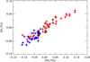 |
Fig. 5. [Ni/Fe] versus [Na/Fe]. Stars are shown with the same symbols as in Fig. 3. |
| In the text | |
|
Fig. 6. Difference between oxygen abundances derived from the 7774 Å O I triplet and the [O I] 6300 Å line versus [Fe/H] after applying 3D non-LTE corrections from Amarsi et al. (2019b). The full drawn line is a least-squares fit to the data. |
| In the text | |
|
Fig. 7. Comparison of Ti and Cr abundances derived from lines belonging to the neutral and ionised species. |
| In the text | |
|
Fig. 8. C/O number ratio as a function of stellar age with blue and red filled circles referring to the two sequences Fig. 3. Stars for which one or more planets have been detected are labelled with a black ring. |
| In the text | |
|
Fig. 9. [Y/Mg] versus stellar age with the same symbols as in Fig. 3. The line corresponds to the linear fit given in Eq. (6). |
| In the text | |
|
Fig. 10. Deviations of [Y/Mg] from Eq. (6) as a function of [Fe/H]. The line shows a linear fit to the data. |
| In the text | |
|
Fig. 11. [Sr/Mg] versus stellar age with the same symbols as in Fig. 3. The line shows the linear fit given in Eq. (7). |
| In the text | |
|
Fig. 12. Deviations of [Sr/Mg] from Eq. (7) as a function of [Fe/H]. The line shows the linear fit to the data. |
| In the text | |
|
Fig. 13. HARPS spectrum of ζ1 Ret (blue line) around the Y II line at 5087.4 Å in comparison with the HARPS spectrum of HD 20619 (red line). The lower panel shows the difference ζ1 Ret – HD 20619. |
| In the text | |
|
Fig. 14. ζ1 and ζ2 Ret in the log (L/Lsun) versus Teff diagram in comparison with ASTEC isochrones ranging in age from 0 to 10 Gyr in steps of 1 Gyr. The full drawn lines refer to isochrones interpolated to the surface heavy element abundance of ζ1, Zs = 0.0122, and the dotted lines to isochrones corresponding to the abundance of ζ2 Ret, Zs = 0.0111. |
| In the text | |
|
Fig. 15. HARPS spectra of ζ1 and ζ2 Ret near the centre of the Ca II K line in comparison with the solar flux HARPS spectrum observed as reflected light from Vesta in 2011. The flux is given relative to the continuum flux in the region of the Ca II H&K lines. |
| In the text | |
|
Fig. 16. Abundance difference between ζ1 and ζ2 Ret as a function of elemental condensation temperature (upper panel) compared to the difference in abundances derived for ζ1 Ret in respectively the high and low activity phases shown in Fig. 15 (lower panel). |
| In the text | |
|
Fig. 17. Age-metallicity diagram for dwarf stars with ages determined from Kepler short-cadence observations of individual oscillation frequencies by Silva Aguirre et al. (2015, 2017). |
| In the text | |
|
Fig. 18. Comparison of the [Fe/H]initial-, [O/Fe]-, and [Mg/Fe]-age relations with predictions from the two-infall chemical evolution model. |
| In the text | |
|
Fig. 19. Toomre diagram for stars on the two age sequences in Fig. 3. Stars on the old age sequence are shown with filled red circles and those on the younger age sequence with filled blue circles. The dotted lines correspond to respectively Vtotal = 50 km s−1 and Vtotal = 100 km s−1. The uncertainty of the velocity components is about 1.5 km s−1, corresponding to the size of the circles. |
| In the text | |
Current usage metrics show cumulative count of Article Views (full-text article views including HTML views, PDF and ePub downloads, according to the available data) and Abstracts Views on Vision4Press platform.
Data correspond to usage on the plateform after 2015. The current usage metrics is available 48-96 hours after online publication and is updated daily on week days.
Initial download of the metrics may take a while.