| Issue |
A&A
Volume 640, August 2020
|
|
|---|---|---|
| Article Number | A99 | |
| Number of page(s) | 12 | |
| Section | Extragalactic astronomy | |
| DOI | https://doi.org/10.1051/0004-6361/202038112 | |
| Published online | 24 August 2020 | |
The soft excess of the NLS1 galaxy Mrk 359 studied with an XMM-Newton-NuSTAR monitoring campaign
1
Dipartimento di Matematica e Fisica, Università degli Studi Roma Tre, via della Vasca Navale 84, 00146 Roma, Italy
e-mail: This email address is being protected from spambots. You need JavaScript enabled to view it.
2
Space Science Data Center, SSDC, ASI, Via del Politecnico snc, 00133 Roma, Italy
3
INAF – Osservatorio Astronomico di Roma, Via Frascati 33, 00040 Monteporzio Catone, Italy
4
Univ. Grenoble Alpes, CNRS, IPAG, 38000 Grenoble, France
5
INAF-Osservatorio di astrofisica e scienza dello spazio di Bologna, Via Piero Gobetti 93/3, 40129 Bologna, Italy
6
INAF/Istituto di Astrofisica e Planetologia Spaziali, Via Fosso del Cavaliere, 00133 Roma, Italy
7
ASI – Unità di Ricerca Scientifica, Via del Politecnico snc, 00133 Roma, Italy
8
Núcleo di Astronomía de la Facultad dei Ingeniería, Universitad Diego Portales, Av. Ejército Libertador 441, Santiago, Chile
Received:
7
April
2020
Accepted:
10
June
2020
Abstract
Context. Joint XMM-Newton and NuSTAR multiple exposures allow us to disentangle the different emission components of active galactic nuclei (AGNs) and to study the evolution of their different spectral features. In this work, we present the timing and spectral properties of five simultaneous XMM-NewtonandNuSTAR observations of the Narrow Line Seyfert 1 galaxy Mrk 359.
Aims. We aim to provide the first broadband spectral modeling of Mrk 359 describing its emission spectrum from the UV up to the hard X-rays.
Methods. We performed temporal and spectral data analysis, characterising the amplitude and spectral changes of the Mrk 359 time series and computing the 2–10 keV normalised excess variance. The spectral broadband modelling assumes the standard hot Comptonising corona and reflection component, while for the soft excess we tested two different models: a warm, optically thick Comptonising corona (the two-corona model) and a reflection model in which the soft-excess is the result of a blurred reflected continuum and line emission (the reflection model).
Results. High and low flux states were observed during the campaign. The former state has a softer spectral shape, while the latter shows a harder one. The photon index is in the 1.75–1.89 range, and only a lower limit to the hot-corona electron temperature can be found. A constant reflection component, likely associated with distant matter, is observed. Regarding the soft excess, we found that among the reflection models we tested, the one providing the better fit (reduced χ2 = 1.14) is the high-density one. However, a significantly better fit (reduced χ2 = 1.08) is found by modelling the soft excess with a warm Comptonisation model.
Conclusions. The present analysis suggests the two-corona model as the best scenario for the optical-UV to X-ray emission spectrum of Mrk 359.
Key words: galaxies: active / galaxies: Seyfert / X-rays: galaxies / X-rays: individuals: Mrk 359
© ESO 2020
1. Introduction
The primary X-ray emission of active galactic nuclei (AGNs) is usually explained by invoking a two-phase scenario (e.g. Haardt & Maraschi 1991, 1993; Haardt et al. 1994) in which thermal electrons (the so-called hot corona) intercept and Comptonise optical-UV photons arising from the accretion disc. Different arguments (timing and microlensing, e.g. Chartas et al. 2009; Morgan et al. 2012; De Marco et al. 2013; Uttley et al. 2014; Kara et al. 2016) support the hot corona to ensure it remains compact and located in the inner regions of the accretion flow. The X-ray primary spectrum is well approximated by a cut-off power law with a photon index (Γhc) in the range of 1.5–2.5 (e.g. Bianchi et al. 2009), and the high-energy rollover (Ec) is interpreted as a further signature of thermal Comptonisation. Such phenomenological quantities depend on the opacity and temperature of the hot corona (e.g. Shapiro et al. 1976; Rybicki & Lightman 1979; Sunyaev & Titarchuk 1980; Beloborodov et al. 1999; Petrucci et al. 2001; Middei et al. 2019a).
Circumnuclear matter can reprocess part of the X-ray continuum, giving rise to an Fe Kα fluorescent emission line (e.g. Bianchi et al. 2009), which is sometimes accompanied by weaker features due to ionised iron (see e.g. Molendi et al. 2003; Bianchi et al. 2005). The neutral Fe Kα emission line has an intrinsically narrow profile. However, Doppler shift and gravitational redshift (due to special and general relativity, respectively) can broaden the line profile, and this effect is stronger when the reflection materials are closer to the supermassive black hole (SMBH, e.g. Fabian et al. 2000; Matt et al. 1993). Additionally, reflection off Compton thick matter gives rise to the so-called Compton hump at about 30 keV (e.g. George & Fabian 1991; Matt et al. 1991, 1993; García et al. 2014; Dauser et al. 2016).
An emission in excess of the extrapolated high-energy power law (e.g. Bianchi et al. 2009; Gliozzi & Williams 2020) is often observed in the soft part (below ∼1–2 keV) of AGNs’ X-ray spectra. The origin of this soft excess is still debated, and different competing models have been proposed to explain it. At present, the two most popular ones are blurred ionised reflection from the innermost regions of the accretion disc (e.g. Miniutti & Fabian 2004; Crummy et al. 2006; Walton et al. 2013; Liebmann et al. 2018), and a warm (kT ∼ 0.5–1 keV), optically thick Comptonising layer above the accretion disc (e.g. Magdziarz et al. 1998; Jin et al. 2012; Done et al. 2012; Petrucci et al. 2013; Kubota & Done 2018; Petrucci et al. 2018, 2020).
The Mrk 359 galaxy (z = 0.0174, Maurogordato et al. 1997) is the first discovered narrow-line Seyfert galaxy (NLS1) (Davidson & Kinman 1978; Osterbrock & Dahari 1983), where the width of the broad emission line is smaller than 2000 km s−1. Elvis et al. (1992) first reported on the X-ray properties of this source in the context of the Einstein Slew Survey. Boller et al. (1996) used ROSAT data to report on the steep soft X-ray emission of Mrk 359 (Γ = 2.4 ± 0.1), while Walter & Fink (1993) claimed the presence of a strong soft X-ray excess. The best knowledge of the X-ray behaviour of this source is derived from an archival XMM-Newton observation (July 2000) analysed by O’Brien et al. (2001). The authors found a power-law-like spectrum with Γ ∼ 1.84 in the 2–10 keV band, a prominent soft X-ray excess and no significant neutral/warm intrinsic absorption. The spectrum showed a noticeable neutral iron emission line (EW ∼ 200 eV) modelled via two components of approximately equal strengths: a broad iron line from an accretion disc and a narrow unresolved line core (EW ∼ 120 eV) consistent with fluorescence from neutral iron in distant reprocessing matter. This AGN was later analysed by Walton et al. (2013), who studied a 2007 Suzaku observation. They modelled the source spectrum with a power-law-like primary continuum and a reflection component computed using REFLIONX (Ross & Fabian 2005). Walton et al. (2013) found the primary photon index to be Γ = 1.90 ± 0.03, and explained the soft excess with a blurred ionised reflection.
In this paper, we report on the XMM-Newton-NuSTAR observational campaign targeting the unobscured AGN. The aim of the campaign was to study the broadband, time-resolved spectra of this source and shed light on the nature of its prominent soft X-ray excess. The standard cosmology ΛCDM with H0 = 70 km s−1 Mpc−1, Ωm = 0.27 and Ωλ = 0.73 is adopted throughout this work.
2. Data reduction
The present dataset consists of five XMM-Newton-NuSTAR simultaneous exposures taken at the beginning of 2019 (see Table 1). Analyses were performed on XMM-Newton-pn/OM and NuSTAR FPMA/B data, while the MOS detectors were not considered due to the lower statistics of their spectra.
Satellite, observation ID, start date, and net exposure time are reported.
The XMM-Newton data were processed using the XMM-Newton Science Analysis System (SAS, Version 18.0.0). The choice of the source extraction radius and the screening for high background time intervals were performed by an iterative process aimed at maximising the signal-to-noise ratio (S/N, details in Piconcelli et al. 2004). For each observation, we obtain the source radius that maximises the S/N ratio. These radii span between 15 and 40 arcsec, where smaller values are used when the background is higher (specifically for observations 1 and 5). At this stage it is worth noting that these different sizes for the extracting regions are taken into account during the computations of the spectra, hence the results of the spectral analysis are not affected. The background was extracted using a 40 arcsec region close to the source. Spectra were binned to have at least 30 counts for each spectral bin, and not to oversample the instrumental energy resolution by a factor larger than three. We notice that no significant pile-up affects the pn data, as also indicated by the SAS task epatplot. Data obtained with the Optical Monitor (Mason et al. 2001, OM) are also used. This telescope on-board XMM-Newton observed Mrk 359 in the UVM2 (2310 Å), UVW1 (2910 Å), and UVW2 (2120 Å) filters, and such measurements are available for all the visits. The OM data were extracted using the on-the-fly data processing and analysis tool RISA, the remote interface SAS analysis and spectral points were converted into a convenient format to be analysed with XspecArnaud (1996) using the standard task om2pha. The OM light curves for the different filters are reported in Fig. 1.
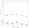 |
Fig. 1. OM light curves for the five observations of the 2019 campaign. The different filters are labelled in the plot. |
In Fig. 2, we show the XMM-Newton/pn average count rates for each observation versus the UVW2 count rate. The correlation between the 0.3–2 keV band and the UVW2 is supported by a Pearson’s correlation coefficient of 0.93 accompanied by a null hypothesis probability of 0.04.
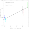 |
Fig. 2. UVW2 rates are shown as a function of the EPIC-pn count rate in the 0.3–2 keV band. The suggestive correlation between these two quantities is supported by the Pearson correlation coefficient and its low null probability reported in the graph. |
The NuSTAR observations were reduced using the standard pipeline (nupipeline) in the NuSTAR Data Analysis Software and by adopting the calibration database x20180710. High-level products were obtained using the nuproducts routine for both the hard X-ray detectors FPMA/B. A 40 arcsec-radius circular region was used to extract the source spectra, while the background was computed from a blank area with the same radius near the source. NuSTAR spectra were then binned to have an S/N greater than three in each spectral channel, and not to oversample the energy resolution by a factor larger than 2.5. The spectra of the whole dataset, unfolded using a Γ = 2 and a common unitary normalisation, are shown in Fig. 3.
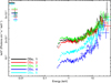 |
Fig. 3. Unfolded spectra (Γ = 2) as observed by XMM-Newton (EPIC-pn and OM) and NuSTAR are presented. The colours black, red, green, blue, and cyan account for visit 1, 2, 3, 4, and 5, respectively. This colour code is applied throughout the whole paper. |
3. Timing properties
The variability of an AGN is stochastic, aperiodic, and ubiquitously observed across the whole electromagnetic spectrum. In X-rays, AGNs not only exhibit long-term amplitude variations (e.g. Vagnetti et al. 2011, 2016; Paolillo et al. 2017; Gallo et al. 2018), but also show rapid changes down to ks timescales (e.g. Ponti et al. 2012).
During the monitoring, Mrk 359 varied both within and among the observations (see Fig. 4). In accordance with Fig. 4, we can define two different flux states in the XMM-Newton bands: a high one in visits 1, 2, and 3, and a low one (counts decrease by a factor of ∼3) in the fourth and fifth observations. In Fig. 4, the two flux regimes are emphasised by the horizontal violet solid line, which indicates the average count rate of that specific observation in that band. Interestingly, UVM2 and UVW2 counts drop between observation 3 and 4 (see Fig. 1).
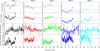 |
Fig. 4. XMM-Newton light curves (background subtracted) in the 0.3–2 keV and 2–10 keV energy bands are shown in the top and top-middle panels, respectively. Bottom-middle panels: NuSTAR background subtracted light curves in the 10–79 keV band are reported, while the bottom row reports on the ratios between light curves in the 0.3–2 keV and 2–10 keV band. The adopted time binning is 1 ks for all the observations, and the solid violet lines account for the average rate of each observation, while dashed lines account for the standard error of the mean. |
Flux variations are observed at timescales as short as a few ks both in the soft and hard X-ray bands. The largest amplitude variation occurs in observation 3, where the soft X-ray emission increases by a factor of ∼3 in under 50 ks. NuSTAR light curves show a similar variability, though, in this high-energy band, the presence of the two flux regimes seen in the XMM-Newton data is not observed.
In Fig. 4, we also show the ratios of the (0.3–2 keV) and (2–10 keV) bands for the pn data. The hardness ratios do not exhibit strong changes within each pointing, hence, we decided to use the time-averaged spectrum for the forthcoming spectral analysis. Ratios show that the source spectrum is hardening in observations 4 and 5 with respect to visits 1, 2, and 3 and this further supports the change of state during the campaign.
As reported by several authors, the amount of X-ray variability at short timescales is anti-correlated with the AGN’s luminosity (e.g. Barr & Mushotzky 1986; Green et al. 1993; Lawrence & Papadakis 1993; Ponti et al. 2012), and the same behaviour has been found at longer timescales (e.g. Markowitz & Edelson 2001; Vagnetti et al. 2011, 2016). On the other hand, such an anti-correlation has been explained as a by product of a more intrinsic relation between the variability and SMBH mass itself (e.g. Papadakis 2004; McHardy et al. 2006; Körding et al. 2007). For these reasons, X-ray amplitude variations can be used to weight the SMBH mass. Following the prescriptions of Ponti et al. (2012), we computed the normalised excess variance (e.g. Nandra et al. 1997; Vaughan et al. 2003). This estimator can be defined as  , where S2 and σn account for the variance and mean square uncertainties of the fluxes, while ⟨f⟩ is the unweighted mean of the flux. Adopting a 250 s time bin for estimating the light curves and selecting 20 ks-long segments, we computed the normalised excess variance in the 2–10 keV band to be
  . Then, following the relations presented by Ponti et al. (2012), we estimate the Mrk 359 BH mass to be MBH = (3.6 ± 1.4)×106 M⊙.
Such a variability-based estimate is consistent within the errors with the BH mass of MBH = 1.7 × 10⁶ M⊙ measured by Wang & Lu (2001), who computed the stellar velocity dispersion σ⋆ via the [O III]. Our estimate is also marginally compatible with what has been found by Williams et al. (2018) based on the X-ray scaling method (firstly discussed in Gliozzi et al. 2011). However, the above quoted measures are larger than the one by Botte et al. (2005), who obtained MBH = 6.9 × 10⁵ M⊙ via a [Ca II] absorption triplet-based stellar velocity dispersion.
We adopt our BH mass estimate to compute the bolometric luminosity and the Eddington ratio of Mrk 359. In particular, we relied on the bolometric correction described by Duras et al. (2020). Such a bolometric correction was calibrated by fitting the spectral energy distribution of ∼1000 unobscured and obscured AGNs (type 1 and 2, respectively) of which luminosities cover six orders of magnitude. Following their paper and using an average 2–10 keV luminosity of 3 × 1042 erg s−1, we obtain log(LBol/erg s−1) = 43.6 and an Eddington ratio of log(LBol/LEdd) ≈ 8%.
We further exploited the current data set by computing the fractional root mean square variability amplitude (Fvar) for each observation of the monitoring (e.g. Edelson et al. 2002). Such a variability estimator is defined as the square root of the normalised excess variance and it has been widely adopted in literature (e.g. Vaughan et al. 2004; Ponti et al. 2006; Matzeu et al. 2016a,b, 2017; Alston et al. 2019; Parker et al. 2020; De Marco et al. 2020; Igo et al. 2020). We compute Fvar following Vaughan et al. (2003) and using the background subtracted pn light curves with a temporal bin of 2500 s. The obtained Fvar are shown in Fig. 5 as a function of the energy. These variability spectra further strengthen the idea of two different states: one less variable and corresponding to the higher flux state of observations 1, 2, and 3, and the other being characterised by larger variability and corresponding to the lower flux observations 4 and 5. Interestingly, the decrease of variability with luminosity is naturally explained if the process results by the superposition of N randomly emitting sub-units. Such a scenario, already considered for optical analyses (e.g. Pica & Smith 1983; Aretxaga et al. 1997), predicts a variability amplitude ∝N−0.5 ∝ L−0.5 when, in its simplified 0-th order version, the sub-units are identical and flare independently (e.g. Green et al. 1993; Nandra et al. 1997; Almaini et al. 2000). In the X-ray band, such a behaviour has been reported by many authors, both for local and high-redshift AGNs (e.g. Barr & Mushotzky 1986; Lawrence & Papadakis 1993; Papadakis et al. 2008; Vagnetti et al. 2011, 2016). In accordance with Fig. 5, the different spectral bands vary in a similar amount, at least for the observations 1, 2, and 3, while in observations 4 and 5, the soft X-ray band may have larger variability. As a final test, we searched for correlations between light curves at different energies or, in other words, we checked if the light curves at different energies varied in concert or not. In particular, we extracted the background subtracted light curves in the 0.5–2, 2.5–5 and 8–10 keV bands, these intervals likely being dominated by different emitting components, the soft excess, the primary continuum, and the reflected component. We therefore computed the Pearson cross-correlation coefficient for the different light curves, finding a strong correlation between the 0.5–2 and 2.5–5 keV bands (Pcc = 0.91, P(r < 0) < 10−22) and a moderate correlation between the 2.5–5 and 8–10 keV bands (Pcc = 0.74, P(r < 0) < 10−15). Finally, the 0.5–2 keV light curve and the 8–10 keV one are only weakly correlated, as supported by a Pcc = 0.42, P(r < 0) = 10−6.
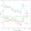 |
Fig. 5. Fractional variability spectra for the different observations. Observations 1, 2, and 3 show smaller variability with respect to observations 4 and 5. Error bars account for 1σ uncertainty. |
4. Spectral analysis
In the fits, the Galactic hydrogen column density NH = 4.38 × 1020 cm−2 (HI4PI Collaboration et al. 2016) is always included and kept frozen to the quoted value. When OM data are analysed, extinction is taken into account with the redden model in XSPEC. We used RB − V = 0.0468 (Schlafly & Finkbeiner 2011), and we kept this value fixed during the computations.
4.1. Primary emission and its reflected component
We started to focus on the Fe Kα properties only using pn data, and ignoring spectra below 3 keV. We adopted a power law to fit the 3–10 keV spectra, with the model parameters untied between the observations and free to vary. This crude fit, only accounting for the primary continuum, returns a χ2 = 525 for 458 degrees of freedom (d.o.f.). This is mainly due to the prominent emission line at about 6.4 keV, see Fig. 6. To model such residuals, we add a Gaussian component. We therefore tested the model: tbabs×(power-law+zgauss) in which the line energy centroid, its width, and normalisation were free to vary in all the observations. However, this preliminary fit shows that in none of the pointings is the line resolved (see Fig. 7), thus for the forthcoming fits, we fixed the line width to zero. A value of χ2 = 443 for 448 d.o.f characterises our model and the corresponding best fit parameters are reported in Table 2. The Fe Kα fluorescent emission-line intensity is consistent with being constant over the campaign. This, together with the narrow profile, suggests an origin from material far from the nuclear region.
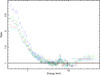 |
Fig. 6. Joint XMM-Newton-NuSTAR spectra with respect to a power-law modelling in the 3–10 keV band. A remarkable soft excess rises smoothly below 2–3 keV above the extrapolated 3–10 keV power law in all the observations. Moreover, it exhibits strong variability. In the Fe K energy band, a strong emission line is apparent, while in hard X-rays, residuals show a Compton hump. |
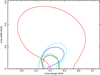 |
Fig. 7. Confidence contours at 90% (two significant parameters) confidence levels for the Fe Kα energy centroid and line intrinsic width. The Fe Kα width is consistent with zero in all the observations. |
Best fit parameters for the 3–10 keV XMM-Newton data and for the 3–79 keV joint pn and FPMA/B data.
To constrain and understand the nature of the reprocessed emission in Mrk 359, we added the NuSTAR FPMA/B 3–79 keV data. The EPIC-pn spectra showed the Fe Kα to be constant and narrow, likely originating from Compton-thick cold material far from the SMBH. Therefore, we studied the 3–79 keV spectra using a cut-off power law to account for the source’s primary continuum and xillver (García et al. 2014; Dauser et al. 2016) to reproduce the neutral Fe Kα line and its associated reflection spectrum. In the fit, we left the high-energy cut off and the primary normalisation untied and free to vary between the observations the photon index. Xillver’s continuum parameters are tied to those of the cut-off power law, with the exception of the normalisation, which is set as free to vary in each observation. The Fe abundance is fitted by tying its value among the pointings, while the ionisation parameter is fixed to log(ξ/erg s−1 cm) = 1 (close to neutral). To account for the inter-calibration between the detectors, we include a free constant. The two NuSTAR modules are in good agreement with each other (∼3%), and they agree with pn data within ≲7% in all but the fourth observation, for which a value of about 30% is found. Such a high value is due to the flux increase caught by NuSTAR only (see the blue light curves in Fig. 4). We re-extracted the NuSTAR spectra in order to be truly simultaneous with XMM-Newton. Once truly simultaneous XMM-Newton/NuSTAR data are considered, the different instruments are consistent with each other within ∼5%, thus, in the subsequent analysis, we used these truly simultaneous spectra.
These steps lead to a best fit with χ2 = 1298 for 1242 d.o.f., see Fig. 8. In Table 2, we report the corresponding best fit values. We notice that this model yields higher values for the photon index of the nuclear emission now being in the range 1.68–1.82. Though the photon indices are fairly consistent within the errors, the overall scenario is consistent with the softer when brighter behaviour, in agreement with what commonly observed in nearby Seyfert galaxies (e.g. Sobolewska & Papadakis 2009) or in AGNs samples (e.g. Serafinelli et al. 2017). The high-energy cut off (Ec) is unconstrained, and the higher value for its lower limits is Ec > 220 keV, found in observation 3. To further assess the constancy of the reflected emission in Mrk 359, we tied the xillver normalisation among the observations. Moreover, we also try to fit the high-energy cut off tying its value between the pointings. This procedure returns a fit of χ2 = 1302 for 1250. Only a lower limit is found for the high-energy cut off (Ec > 340 keV). The model xillver normalisation is Nrefl = (1.5 ± 0.3)×10−5 photons keV−1 cm−2 s−1 with an associated flux F3−79 keV = (8.7 ± 1.4)×10−13 erg s−1 cm−2.
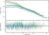 |
Fig. 8. Best fit to the 3–79 keV XMM-Newton-NuSTAR data corresponding to the model (tbabs×cutoffpl×xillver). χ2/d.o.f. = 1.04. |
4.2. Broadband data: testing the two-corona model
At this stage of the analysis, we include OM spectral points and pn data down to 0.3 keV. Two Comptonising components, one optically thick and warm (warm corona, wc) and the other optically thin and hot (hot corona, hc), have often been used to reproduce broadband AGN spectra (e.g. Porquet et al. 2018; Middei et al. 2018, 2019b; Ursini et al. 2018, 2020; Noda & Done 2018; Kubota & Done 2018; Petrucci et al. 2018; Matzeu et al. 2020), therefore we tested the so-called two-corona model on the present dataset. In Xspec, such a model appears as:
redden× TBabs× const×
×[smallBB+ nthcompwc+nthcomphc+xillvercp].
The smallBB component accounts for the broad-line region (BLR), and in particular for the so-called small blue bump (SBB) at about 3000 Å, as described in detail in Mehdipour et al. (2015). By fitting this component (kept tied among the pointings), we find its flux to be F = 4.5 × 10⁻¹² erg cm2 s−1. Nthcompwc (Zdziarski et al. 1996; Życki et al. 1999) provides a thermally Comptonised continuum whose high- and low-energy rollovers are parametrised by the temperatures of the electrons (kTwc) and the seed photons (kTbb). We assumed the seed photons to arise from a disc blackbody, and we fitted the kTbb parameter by tying its value between the various observations. The photon index (Γwc), the warm corona’s temperature, and the normalisation are considered as free parameters in all the observations. Then, nthcomphc and xillvercp are used to reproduce the high-energy emission of Mrk 359. The first model accounts for the primary Comptonised power law, the latter for its associated reflected component. Disc photons accounted by nthcomphc are assumed to arise from the same disc-like blackbody feeding the warm corona, thus we tied the kTbb to the one in nthcompwc. To model the hot component, we fitted the primary photon index (Γhc), the electrons temperature kThc, and normalisation in all the observations. The normalisation of xillvercp is free for all the visits of the campaign, while the ionisation degree and the iron abundance are free to vary but tied among the different observations.
Such a procedure yields the data best fit (χ2 = 1690 for 1567 d.o.f.) shown in the left panel of Fig. 9. The contribution of the two coronae to the fit is shown in the right panel of Fig. 9. The best fit values for the parameters are reported in Table 3. The fit returns an iron abundance AFe = 1.3 ± 0.3 and an ionisation parameter of log(ξ/erg s−1 cm) = 1.33 ± 0.05. Using the best fit values for the coronal temperature and the photon index, we derived the opacity of the two coronae1. The photon index of the warm component varies in the range 2.46–2.69 and higher values of Γwc are measured when the component flux decreases, see top panel of Fig. 10. Concerning the hot corona, the photon index shows weak changes (1.75 ≤ Γhc ≤ 1.88) and only lower limits are found for the hot corona’s temperature. Opposite to what we found for the warm corona, steeper Γhc correspond to brighter states. For both coronae, we show the contours between the photon index Γwc/hc and the electron temperature kTwc/hc in Fig. 11.
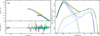 |
Fig. 9. Left panel: optical-UV to hard X-rays fitted with the two-corona model (χ2 = 1690 for 1567 d.o.f.). Right panel: underlying best fit model is shown by the solid lines, while dashed ones account for the contribution of each of the two coronae. |
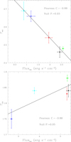 |
Fig. 10. Top panel: Γwc as a function of the warm Comptonisation flux estimated in the 0.3–2 keV. Bottom panel: the same as for the hot corona, for which the flux has been computed in the 2–10 keV band. Fluxes are in units of 10−12 erg s−1 cm−2. |
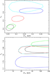 |
Fig. 11. Contours at 90% confidence level (Δχ2 = 4.61) between the primary continuum photon index and the temperature for both the warm corona (top panel) and the hot corona (bottom panel). The temperature of the hot corona remains unconstrained, and only lower limits are obtained. The photon indices of both components change from one observation to the other. |
Best fit parameters for the two-corona model.
4.3. Broadband data: testing relativistic reflection
A weak or negligible broad component of the Fe Kα emission line may still allow for a prominent relativistic reflection continuum. For this reason, we investigated whether a blurred ionised reflection could be responsible for the soft excess in Mrk 359. Here, we modify the two-corona model presented in Sect. 4.2, replacing nthcompwc with relxillcp (Dauser et al. 2014, 2016). Such a model calculates a standard relativistic reflection spectrum resulting from a Comptonised continuum irradiating the accretion disc. Moreover, we account for the accretion disc emission including a diskbb component. Therefore, we use the following model:
redden× TBabs× const×
× [smallBB+diskbb+nthcomp+relxillcp+xillvercp].
Nthcomp still provides the primary continuum emission, and we calculated the photon index, the electron temperature, and the normalisation in all the pointings. The nthcomp seed photons temperature is the same as diskbb, thus we tied this parameter between the two components. The current dataset does not provide any constrain on this temperature, and we set its value to be consistent with what was previously found for the two-corona model. The normalisation of the diskbb component is free to vary in all observations. We use the smallBB table to account for the SBB also in the current model. During the fitting procedure, the table’s normalisation was tied between the observations. After fitting the whole dataset, for this component we obtain a flux of ∼4 ×10⁻¹² erg cm−2 s−1. Relxillcp and xillvercp were used to reproduce the reflected continuum only, hence we fitted the models’ normalisations in each pointing. Relxillcp allows for spin (a) estimates, though after a preliminary fit we find this parameter to be consistent with a > 0.985. For this reason, we assumed the SMBH to be maximally rotating and we left the inner radius free to vary in all the pointings. The iron abundance of the reflecting material is free to vary and tied between the reflection models and the observations. We also fitted the ionisation degree of the relativistic reflection component and that of xillvercp. Such a procedure returns a fit with a value of χ2/d.o.f. = 2087/1568, with large residuals mainly in the soft X-ray band (see top row in Fig. 12). As a subsequent step, we allowed the corona emissivity q and the inclination parameter i to vary. The inclination is tied between xillvercp and relxillcp. The addition of these two parameters is beneficial in terms of statistical quality (Δχ2/Δ d.o.f. = −253/−2), and we get an overall fit characterised by χ2/d.o.f. = 1834/1566. In Table 4, the fitted values are shown. The current model returns a slightly supersolar iron abundance AFe = 1.55 ± 0.25, and a log(ξ/erg s−1 cm) = 2.72 ± 0.04 is required to reproduce the source soft-excess. The model returns a disc inclination of i = 71 ± 1 deg and the inner disc region is consistent with a few gravitational radii. Reflection due to distant matter is compatible with being constant and likely due to almost neutral material log(ξ/erg s−1 cm) = 0.15 ± 0.12. The primary continuum can be described by a power law of which Γ varies between 1.92 and 2.03, while the electron temperature is kT>140 keV. We notice that these photon indices are steeper and not consistent with those obtained in the two-corona model. Relxillcp also allows for a broken power-law emissivity profile of the primary continuum emission (q2). However, the assumption of such a different emissivity profile has a negligible impact in terms of statistical quality and q2 > 1.3 is found.
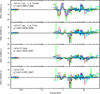 |
Fig. 12. Contribution to the χ2 in each bin for the different relativistic models tested in Sect. 4.3. We recall the corresponding model in each panel’s row, and for the first and the second rows we also specify some of the frozen or free parameters. |
Different Relxill versions have been published (e.g. Dauser et al. 2016) and each of them accounts for a specific physical and geometrical corona-disc scenario. Therefore, we further tested the relativistic reflection scenario, replacing relxillcp with relxilllpcp, which accounts for a lamp-post corona-SMBH geometry. In this model, it is possible to fit the height (h, in units of gravitational radii rg) of the hot corona above the accretion disc, which is split into multiple zones, with each of them seeing a different incident spectrum due to relativistic energy shifts of the nuclear continuum. The fitting procedure is similar to the one described for the case of relxillcp, and we calculated the coronal height above the accretion disc by tying its value among the pointings. The fit returns h = 6.3 ± 0.5 rg, but the corresponding statistical quality is worse with respect to the previous test as we find χ2/d.o.f. = 1915/1567. The primary continuum is characterised by changes in the source spectral shape, and the obtained values are slightly steeper with respect to those previously computed with relxillcp. A sub-solar value of AFe = 0.55 ± 0.05 is obtained. The ionisation parameter for the relativistic reflection component is log(ξ/erg s−1 cm) = 2.88 ± 0.04, while for xillvercp we get log(ξ/erg s−1 cm) = 0.03 ± 0.01. The current fit returns a well-constrained disc inclination, though its value is extreme at i = 84 ± 1 deg. As a last attempt, we left the corona height free to vary between the observations. However, no statistically significant variability of h is found.
Finally, we tested the high-density version of relxill, which is relxillD (Dauser et al. 2016, high density model in Table 4). Such a model allows for the density of the accretion disc to vary in the 15–19 range, where the standard version of the reflection code assumes this quantity to be log(ρ/cm−3) = 15. However, in its current version, relxillD does not allow for a variable high -energy cut off that is assumed to be frozen at 300 keV. Once relxillcp had been replaced with its high-density counterpart, we fitted ρ, tying its value between the different observations, while the other parameters were treated as in case of relxillcp. The fit to the data returns a disc-density value of log(ρ/cm−3) = 18.05 ± 0.03, the other parameters being marginally affected by this new model and consistent within the errors with what was previously obtained, with the exception of the ionisation parameter for the relativistic component found to be log(ξ/erg s−1 cm) = 1.3 ± 0.1: much smaller than in previous fits. This model is better on statistical grounds (χ2 = 1789 for 1567 d.o.f.) than the previously tested reflection models. Also, for this modelling the iron abundance is sub-solar (AFe = 0.70 ± 0.08). In this case, the corona emissivity is not compatible with what was previously estimated by relxillcp since the fit gives q = 2.15 ± 0.10 for this parameters, while an extreme disc inclination of i = 83 ± 1 deg is found.
The best fit parameters for all the models tested in this section are reported in Table 4. In accordance with our tests, relxillD provides the most satisfactory fit among the relativistic reflection models, though the emerging scenario is characterised by a large disc inclination.
5. Summary and conclusions
In this section, we first summarise the results of the present analysis, and then propose a possible scenario.
5.1. Results
We presented the UV-to-X-ray spectral characterisation of Mrk 359, the first discovered NLSy1. Data belong to a monitoring campaign of 5 × 50 ks XMM-Newton-NuSTAR simultaneous exposures taken every ∼2 days, see Table 1. In the following, we highlight the main findings of this work:
-
The Seyfert galaxy Mrk 359 varied on different timescales and spectral bands as shown in Fig. 4. In fact, amplitude changes up to a factor of ≲3 occurred in the XMM-Newton 0.3–2 and 2–10 keV bands, as well as in the harder NuSTAR bandpass. Interestingly, the XMM-Newton light curves computed for the first three observations are a factor of ∼3 higher with respect to the fourth and fifth pointings, and a similar behaviour seems to characterise the OM UVM2 and UVW2 filters (see Fig. 1). The suggestive correlation between UV photons and the soft X-ray band is shown in Fig 2, and this is in agreement with what is expected from the two-corona model. Hardness ratios between the 0.3–2 and 2–10 keV bands are weakly variable within the same pointing, though spectral changes are observed between the different exposures. The light curves shown in Fig. 4 are consistent with the “softer when brighter” behaviour (e.g. Bianchi et al. 2009; Sobolewska & Papadakis 2009; Serafinelli et al. 2017), meaning that harder spectral states correspond to lower fluxes.
-
The Fvar spectra are in agreement with two variability states Mrk 359 underwent during the monitoring; observations 1, 2, and 3 are indeed characterised by smaller amplitude variability with respect to observations 4 and 5. Though limited in terms of S/N, the Fvar spectra may suggest that about the same amount of variability occurs over the different energy intervals. The only exception may be observations 4 and 5, for which the soft X-ray band seems to have larger Fvar values.
-
We extracted the EPIC-pn light curves in different energy intervals (0.5–2, 2.5–5 and 8–10 keV) to investigate whether these light curves vary in concert. Such bands, in fact, are likely dominated by three different spectral components: the soft-excess, the primary continuum, and the reflected emission. Based on the Pearson cross-correlation analysis, we find that the strong correlation Pcc = 0.91, P(r < 0) < 10−22 holds between the 0.5–2 and 2.5–5 light curves, while weaker correlation (also in term of statistics) characterises the light curves in the soft X-ray band and the 8–10 keV one (Pcc = 0.42, P(r < 0) < 10−6). Such a result is not consistent with the scenario in which the soft excess is due to relativistic lines blurring, since the reflection component would be present in both energy bands and a correlation would be expected.
-
Using the 2–10 keV band, we quantified the amount of variability in Mrk 359 computing the normalised excess variance (see Sect. 3 for details) that we also used it to estimate Mrk 359 SMBH mass. Following the prescriptions by Ponti et al. (2012), we found MBH = (3.6 ± 1.4)×106 M⊙.
-
The 3–79 keV spectra of Mrk 359 are well described by a power-law-like emission with a Γhc varying between 1.75 and 1.88 and a high-energy cut off Ec > 220 keV, see Table 2. This primary continuum emission is accompanied by a neutral Fe Kα emission line (EW ∼ 90 eV). Such a feature has a width consistent with zero throughout the campaign (see Fig. 7), with no variability observed. NuSTAR data show a more constant behaviour during the campaign and are characterised by the Compton hump shown in Fig. 6. The flux of the reprocessed emission is constant during the monitoring, and the origin of this component is consistent with Compton-thick and cold matter (as commonly found in other Seyfert galaxies, see e.g. Bianchi et al. 2009; Cappi et al. 2016).
-
We fit the broadband UV-to-X-ray emission spectrum of Mrk 359 with two different models: a two-corona model and relativistic reflection. The first model is favoured on statistical grounds and is characterised by a hot component (kThc > 55 keV, τtc < 4.3), which accounts for the primary continuum, and a warmer one (kTwc ∼ 0.3 keV, 20 ≤ τWC ≤ 29) responsible for the UV and soft X-ray emission. The soft-excess can be ascribed to this latter component. Weak/strong spectral variability are observed on the hot/warm phase, as shown in Fig. 11. The relativistic reflection code accounting for a variable density of the accretion disc, relxillD, provides the better fit among the various relxill versions (see also Fig. 12), though its χ2/d.o.f. is significantly larger than that of the two-corona model. It is also worth mentioning that the disc inclination angles obtained with all the relativistic reflection models are fairly extreme, and no evidence of such a large inclination exists for Mrk 359. This also weakens a possible relativistic origin of the soft excess in Mrk 359.
5.2. Two coronae in Mrk 359 and a possible physical scenario
Our analysis shows that the two-corona model is the one that best fits the data, so we discuss it in some detail. The evolution of the physical parameters (optical depth, temperature, photon index) of the two coronae can be used to derive a tentative scenario of the spectral behaviour of the source observed during the campaign.
Following Petrucci et al. (2020), we can estimate the amplification factors for the two coronae. We find Awc < 1.1 and Ahc ∼ 7 for the warm and hot coronas, respectively. The large amplification factor of the hot corona is commonly found in AGNs and is consistent with a scenario in which the seed photons that are Comptonised represent only a small fraction of the photons produced by the accretion disc. This supports geometries like a patchy corona, or a corona inside a truncated disc, or a corona on the SMBH axis (i.e. the so-called lamp-post model). On the other hand, in the case of the warm corona, the value of the temperature and spectral index agree with an amplification factor of ∼1.1, which is consistent with the corona covering a quasi-passive accretion disc. This is shown in Fig. 13, where we report the hot and warm corona’s properties in the spectral photon index versus the temperature plane. This figure is similar to the one discussed in Petrucci et al. (2018, Fig. 1), but it was corrected in Petrucci et al. (2020, Fig. 8). In fact, concerning the warm corona, the five observations are located in two slightly different regions. Observations 1, 2, and 3 have harder warm-corona spectra and are located below the passive disc line, while observations 4 and 5 are above this line (due to their softer warm-corona spectra). This clearly suggests a change of the warm-corona radiative equilibrium during the beginning and the end of the monitoring. Interestingly, observations 1, 2, and 3 have a higher flux than observations 4 and 5, indicating that this change of the warm-corona radiative equilibrium could go with a change of the source flux state.
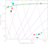 |
Fig. 13. For each observation, Γ and kT of the two coronae are shown. The solid lines refer to the corona optical depth τ (red), the amplification factor A (in blue) and the minimal fraction (in %) of disc intrinsic emission (dark green). Warm corona points lie both below (observations 1, 2, and 3) and above (observations 4 and 5) the zero intrinsic-disc emission line, and this agrees with a change of radiative equilibrium for this component (see Petrucci et al. 2020, for a detailed discussion). |
A tentative scenario to explain the observed spectral variability of Mrk 359 could be the following: assuming a hot corona/truncated-disc geometry where the outer disc is covered by a warm corona, the warm corona’s photons may then enter and cool the hot corona through Comptonisation. This is indeed supported by the suggestive correlation between the hard and soft X-ray flux reported in Fig. 14. We may also assume that the two flux regimes observed during the campaign are the result of a change in the accretion rate ṁ (i.e. the accretion rate slightly decreases between the beginning and the end of the monitoring), and that this change of ṁ goes along with a change of the truncation radius Rtr. In fact, such a relation between ṁ and Rtr is expected in the disc evaporation model developed by, for example, Meyer et al. (2000) and Różańska & Czerny (2000) (see also Czerny & Naddaf Moghaddam 2018, for a review). In this approach, this inner hot corona is fed by matter from the outer thin disc, which evaporates from the cool layers underneath, the evaporation process resulting from thermal instabilities led by the sharp temperature gradient between the hot corona and the outer disc. The warm corona, at the surface of the accretion disc, could be a natural product of this evaporation process. Now the strong dependence of the cooling efficiency on density leads to an anti-correlation between the accretion rate and the truncated radius. So, in this framework, the apparent decrease of the accretion rate during the campaign of Mrk 359 would go along with an increase of the truncation radius. This would mean that fewer photons coming from the outer accretion flow will enter and cool the hot corona, decreasing the cooling process, and resulting in a hardening of its spectrum as observed (see Fig. 10, bottom). On the other hand, the decrease in the accretion rate and increase in the truncation radius will naturally decrease the intrinsic warm corona heating power, as well as the illumination from the hot corona. As a consequence, the warm-corona spectrum would soften in agreement with the observations (see Fig. 10, top). We note that this approach supposes small and local variation timescales of the accretion rate and the truncation radius. This is similar to the case of HE 1143-1810 (Ursini et al. 2020), an AGN that behaves similarly to Mrk 359 in X-rays. These timescales are much shorter (< day) than the viscous timescale needed to reach the ISCO (innermost stable circular orbit) from the truncation radius, and this agrees quite well with the variability timescales observed in our monitoring.
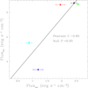 |
Fig. 14. Correlation between flux of the hot Comptonisation component in the 2–10 keV band and the soft one estimated in the 0.3–2 keV band. Fluxes are in units of 10−12 erg s−1 cm−2. |
While this scenario appears to be in qualitative agreement with the observed spectral behaviour of Mrk 359, it is not entirely satisfactory. For example, it does not explain the apparent increase in the warm-corona temperature during the campaign (see Fig. 11), suggesting that other parameters are also playing a role. In any case, better constraints on the truncation radius are needed here to confirm or rule out the present interpretation, and high-resolution instruments that allow highly statistical analyses, like the X-ray Integral Field Unit of the Athena mission (Barret & Cappi 2019; Barret et al. 2020), will be crucial in this respect.
In nthcomp, the medium opacity is related to the photon index Γ of the asymptotic power law and to the temperature θ = kTe/me c2 by the relation τ = 2.25 + 3/[θ × (Γ + 0.5)2 − 2.25]1/2 − 1.5, where the subscript “e” refers to the electron.
Acknowledgments
RM warmly thanks Eleonora Bianchi for being helpful during his time in Grenoble and Fausto Vagnetti, Barbara De Marco & Gabriele Matzeu for useful comments. RM also acknowledges Fondazione Angelo Della Riccia for financial support and Université Grenoble Alpes and the high energy SHERPAS group for welcoming him at IPAG. SB acknowledges financial support from ASI under grants ASI-INAF I/037/12/0 and n. 2017-14-H.O. POP and MCl acknowledges financial support from the CNRS PNHE and from the CNES french agency. This work is based on observations obtained with: the NuSTAR mission, a project led by the California Institute of Technology, managed by the Jet Propulsion Laboratory and funded by NASA; XMM-Newton, an ESA science mission with instruments and contributions directly funded by ESA Member States and the USA (NASA). ADR & MC acknowledge financial contribution from the agreement ASI-INAF n.2017-14-H.O. Part of this work is based on archival data, software or online services provided by the Space Science Data Center - ASI.
References
- Almaini, O., Lawrence, A., Shanks, T., et al. 2000, MNRAS, 315, 325 [NASA ADS] [CrossRef] [Google Scholar]
- Alston, W. N., Fabian, A. C., Buisson, D. J. K., et al. 2019, MNRAS, 482, 2088 [NASA ADS] [CrossRef] [Google Scholar]
- Aretxaga, I., Cid Fernandes, R., & Terlevich, R. J. 1997, MNRAS, 286, 271 [NASA ADS] [CrossRef] [Google Scholar]
- Arnaud, K. A. 1996, Astronomical Data Analysis Software and Systems V, eds. G. H. Jacoby, & J. Barnes, ASP Conf. Ser., 101, 17 [Google Scholar]
- Barr, P., & Mushotzky, R. F. 1986, Nature, 320, 421 [NASA ADS] [CrossRef] [Google Scholar]
- Barret, D., & Cappi, M. 2019, A&A, 628, A5 [NASA ADS] [CrossRef] [EDP Sciences] [Google Scholar]
- Barret, D., Decourchelle, A., Fabian, A., et al. 2020, Astron. Nachr., 341, 224 [NASA ADS] [CrossRef] [Google Scholar]
- Beloborodov, A. M. 1999, in High Energy Processes in Accreting Black Holes, eds. J. Poutanen, & R. Svensson, ASP Conf. Ser., 161, 295 [Google Scholar]
- Bianchi, S., Matt, G., Nicastro, F., Porquet, D., & Dubau, J. 2005, MNRAS, 357, 599 [NASA ADS] [CrossRef] [Google Scholar]
- Bianchi, S., Guainazzi, M., Matt, G., Fonseca Bonilla, N., & Ponti, G. 2009, A&A, 495, 421 [NASA ADS] [CrossRef] [EDP Sciences] [Google Scholar]
- Boller, T., Brandt, W. N., & Fink, H. 1996, A&A, 305, 53 [NASA ADS] [Google Scholar]
- Botte, V., Ciroi, S., di Mille, F., Rafanelli, P., & Romano, A. 2005, MNRAS, 356, 789 [NASA ADS] [CrossRef] [Google Scholar]
- Cappi, M., De Marco, B., Ponti, G., et al. 2016, A&A, 592, A27 [NASA ADS] [CrossRef] [EDP Sciences] [Google Scholar]
- Chartas, G., Kochanek, C. S., Dai, X., Poindexter, S., & Garmire, G. 2009, ApJ, 693, 174 [NASA ADS] [CrossRef] [Google Scholar]
- Crummy, J., Fabian, A. C., Gallo, L., & Ross, R. R. 2006, MNRAS, 365, 1067 [NASA ADS] [CrossRef] [Google Scholar]
- Czerny, B., & Naddaf Moghaddam, M. H. 2018, in Accretion Processes in Cosmic Sources - II, 6 [Google Scholar]
- Dauser, T., García, J., Parker, M. L., Fabian, A. C., & Wilms, J. 2014, MNRAS, 444, L100 [NASA ADS] [CrossRef] [Google Scholar]
- Dauser, T., García, J., Walton, D. J., et al. 2016, A&A, 590, A76 [NASA ADS] [CrossRef] [EDP Sciences] [Google Scholar]
- Davidson, K., & Kinman, T. D. 1978, ApJ, 225, 776 [NASA ADS] [CrossRef] [Google Scholar]
- De Marco, B., Ponti, G., Cappi, M., et al. 2013, MNRAS, 431, 2441 [NASA ADS] [CrossRef] [Google Scholar]
- De Marco, B., Adhikari, T. P., Ponti, G., et al. 2020, A&A, 634, A65 [CrossRef] [EDP Sciences] [Google Scholar]
- Done, C., Davis, S. W., Jin, C., Blaes, O., & Ward, M. 2012, MNRAS, 420, 1848 [NASA ADS] [CrossRef] [Google Scholar]
- Duras, F., Bongiorno, A., Ricci, F., et al. 2020, A&A, 636, A73 [CrossRef] [EDP Sciences] [Google Scholar]
- Edelson, R., Turner, T. J., Pounds, K., et al. 2002, ApJ, 568, 610 [NASA ADS] [CrossRef] [Google Scholar]
- Elvis, M., Plummer, D., Schachter, J., & Fabbiano, G. 1992, ApJS, 80, 257 [NASA ADS] [CrossRef] [Google Scholar]
- Fabian, A. C., Iwasawa, K., Reynolds, C. S., & Young, A. J. 2000, PASP, 112, 1145 [NASA ADS] [CrossRef] [Google Scholar]
- Gallo, L. C., Blue, D. M., Grupe, D., Komossa, S., & Wilkins, D. R. 2018, MNRAS, 478, 2557 [CrossRef] [Google Scholar]
- García, J., Dauser, T., Lohfink, A., et al. 2014, ApJ, 782, 76 [NASA ADS] [CrossRef] [Google Scholar]
- George, I. M., & Fabian, A. C. 1991, MNRAS, 249, 352 [NASA ADS] [CrossRef] [Google Scholar]
- Gliozzi, M., & Williams, J. K. 2020, MNRAS, 491, 532 [CrossRef] [Google Scholar]
- Gliozzi, M., Titarchuk, L., Satyapal, S., Price, D., & Jang, I. 2011, ApJ, 735, 16 [NASA ADS] [CrossRef] [Google Scholar]
- Green, A. R., McHardy, I. M., & Lehto, H. J. 1993, MNRAS, 265, 664 [NASA ADS] [Google Scholar]
- Haardt, F., & Maraschi, L. 1991, ApJ, 380, L51 [NASA ADS] [CrossRef] [Google Scholar]
- Haardt, F., & Maraschi, L. 1993, ApJ, 413, 507 [NASA ADS] [CrossRef] [MathSciNet] [Google Scholar]
- Haardt, F., Maraschi, L., & Ghisellini, G. 1994, ApJ, 432, L95 [NASA ADS] [CrossRef] [Google Scholar]
- HI4PI Collaboration (Ben Bekhti, N., et al.) 2016, A&A, 594, A116 [NASA ADS] [CrossRef] [EDP Sciences] [Google Scholar]
- Igo, Z., Parker, M. L., Matzeu, G. A., et al. 2020, MNRAS, 493, 1088 [CrossRef] [Google Scholar]
- Jin, C., Ward, M., & Done, C. 2012, MNRAS, 425, 907 [NASA ADS] [CrossRef] [Google Scholar]
- Kara, E., Alston, W., & Fabian, A. 2016, Astron. Nachr., 337, 473 [NASA ADS] [CrossRef] [Google Scholar]
- Körding, E. G., Migliari, S., Fender, R., et al. 2007, MNRAS, 380, 301 [NASA ADS] [CrossRef] [Google Scholar]
- Kubota, A., & Done, C. 2018, MNRAS, 480, 1247 [NASA ADS] [CrossRef] [Google Scholar]
- Lawrence, A., & Papadakis, I. 1993, ApJ, 414, L85 [NASA ADS] [CrossRef] [Google Scholar]
- Liebmann, A. C., Fabian, A. C., Tsuruta, S., Haba, Y., & Kunieda, H. 2018, ApJ, 868, 11 [CrossRef] [Google Scholar]
- Magdziarz, P., Blaes, O. M., Zdziarski, A. A., Johnson, W. N., & Smith, D. A. 1998, MNRAS, 301, 179 [NASA ADS] [CrossRef] [Google Scholar]
- Markowitz, A., & Edelson, R. 2001, ApJ, 547, 684 [NASA ADS] [CrossRef] [Google Scholar]
- Mason, K. O., Breeveld, A., Much, R., et al. 2001, A&A, 365, L36 [NASA ADS] [CrossRef] [EDP Sciences] [Google Scholar]
- Matt, G., Perola, G. C., & Piro, L. 1991, A&A, 247, 25 [NASA ADS] [Google Scholar]
- Matt, G., Fabian, A. C., & Ross, R. R. 1993, MNRAS, 262, 179 [NASA ADS] [CrossRef] [Google Scholar]
- Matzeu, G. A., Reeves, J. N., Nardini, E., et al. 2016a, Astron. Nachr., 337, 495 [CrossRef] [Google Scholar]
- Matzeu, G. A., Reeves, J. N., Nardini, E., et al. 2016b, MNRAS, 458, 1311 [NASA ADS] [CrossRef] [Google Scholar]
- Matzeu, G. A., Reeves, J. N., Nardini, E., et al. 2017, MNRAS, 465, 2804 [CrossRef] [Google Scholar]
- Matzeu, G. A., Nardini, E., Parker, M. L., et al. 2020, MNRAS, 497, 2352 [CrossRef] [Google Scholar]
- Maurogordato, S., Proust, D., Cappi, A., Slezak, E., & Martin, J. M. 1997, A&AS, 123, 411 [NASA ADS] [CrossRef] [EDP Sciences] [Google Scholar]
- McHardy, I. M., Koerding, E., Knigge, C., Uttley, P., & Fender, R. P. 2006, NAture, 444, 730 [Google Scholar]
- Mehdipour, M., Kaastra, J. S., Kriss, G. A., et al. 2015, A&A, 575, A22 [NASA ADS] [CrossRef] [EDP Sciences] [Google Scholar]
- Meyer, F., Liu, B. F., & Meyer-Hofmeister, E. 2000, A&A, 361, 175 [NASA ADS] [Google Scholar]
- Middei, R., Bianchi, S., Cappi, M., et al. 2018, A&A, 615, A163 [NASA ADS] [CrossRef] [EDP Sciences] [Google Scholar]
- Middei, R., Bianchi, S., Marinucci, A., et al. 2019a, A&A, 630, A131 [CrossRef] [EDP Sciences] [Google Scholar]
- Middei, R., Bianchi, S., Petrucci, P. O., et al. 2019b, MNRAS, 483, 4695 [NASA ADS] [CrossRef] [Google Scholar]
- Miniutti, G., & Fabian, A. C. 2004, MNRAS, 349, 1435 [NASA ADS] [CrossRef] [Google Scholar]
- Molendi, S., Bianchi, S., & Matt, G. 2003, MNRAS, 343, L1 [NASA ADS] [CrossRef] [Google Scholar]
- Morgan, C. W., Hainline, L. J., Chen, B., et al. 2012, ApJ, 756, 52 [NASA ADS] [CrossRef] [Google Scholar]
- Nandra, K., George, I. M., Mushotzky, R. F., Turner, T. J., & Yaqoob, T. 1997, ApJ, 477, 602 [NASA ADS] [CrossRef] [Google Scholar]
- Noda, H., & Done, C. 2018, MNRAS, 480, 3898 [NASA ADS] [CrossRef] [Google Scholar]
- O’Brien, P. T., Page, K., Reeves, J. N., et al. 2001, MNRAS, 327, L37 [NASA ADS] [CrossRef] [Google Scholar]
- Osterbrock, D. E., & Dahari, O. 1983, ApJ, 273, 478 [Google Scholar]
- Paolillo, M., Papadakis, I., Brandt, W. N., et al. 2017, MNRAS, 471, 4398 [NASA ADS] [CrossRef] [Google Scholar]
- Papadakis, I. E. 2004, MNRAS, 348, 207 [NASA ADS] [CrossRef] [Google Scholar]
- Papadakis, I. E., Chatzopoulos, E., Athanasiadis, D., Markowitz, A., & Georgantopoulos, I. 2008, A&A, 487, 475 [NASA ADS] [CrossRef] [EDP Sciences] [Google Scholar]
- Parker, M. L., Alston, W. N., Igo, Z., & Fabian, A. C. 2020, MNRAS, 492, 1363 [NASA ADS] [CrossRef] [Google Scholar]
- Petrucci, P. O., Haardt, F., Maraschi, L., et al. 2001, ApJ, 556, 716 [NASA ADS] [CrossRef] [Google Scholar]
- Petrucci, P. O., Paltani, S., Malzac, J., et al. 2013, A&A, 549, A73 [NASA ADS] [CrossRef] [EDP Sciences] [Google Scholar]
- Petrucci, P.-O., Ursini, F., De Rosa, A., et al. 2018, A&A, 611, A59 [NASA ADS] [CrossRef] [EDP Sciences] [Google Scholar]
- Petrucci, P. O., Gronkiewicz, D., & Rozanska, A. 2020, A&A, 634, A85 [CrossRef] [EDP Sciences] [Google Scholar]
- Pica, A. J., & Smith, A. G. 1983, ApJ, 272, 11 [NASA ADS] [CrossRef] [Google Scholar]
- Piconcelli, E., Jimenez-Bailón, E., Guainazzi, M., et al. 2004, MNRAS, 351, 161 [NASA ADS] [CrossRef] [Google Scholar]
- Ponti, G., Miniutti, G., Cappi, M., et al. 2006, MNRAS, 368, 903 [NASA ADS] [CrossRef] [Google Scholar]
- Ponti, G., Papadakis, I., Bianchi, S., et al. 2012, A&A, 542, A83 [NASA ADS] [CrossRef] [EDP Sciences] [Google Scholar]
- Porquet, D., Reeves, J. N., Matt, G., et al. 2018, A&A, 609, A42 [NASA ADS] [CrossRef] [EDP Sciences] [Google Scholar]
- Ross, R. R., & Fabian, A. C. 2005, MNRAS, 358, 211 [Google Scholar]
- Różańska, A., & Czerny, B. 2000, A&A, 360, 1170 [NASA ADS] [Google Scholar]
- Rybicki, G. B., & Lightman, A. P. 1979, Radiative Processes in Astrophysics [Google Scholar]
- Schlafly, E. F., & Finkbeiner, D. P. 2011, ApJ, 737, 103 [NASA ADS] [CrossRef] [Google Scholar]
- Serafinelli, R., Vagnetti, F., & Middei, R. 2017, A&A, 600, A101 [NASA ADS] [CrossRef] [EDP Sciences] [Google Scholar]
- Shapiro, S. L., Lightman, A. P., & Eardley, D. M. 1976, ApJ, 204, 187 [NASA ADS] [CrossRef] [Google Scholar]
- Sobolewska, M. A., & Papadakis, I. E. 2009, MNRAS, 399, 1597 [NASA ADS] [CrossRef] [Google Scholar]
- Sunyaev, R. A., & Titarchuk, L. G. 1980, A&A, 86, 121 [NASA ADS] [Google Scholar]
- Ursini, F., Petrucci, P. O., Bianchi, S., et al. 2020, A&A, 634, A92 [CrossRef] [EDP Sciences] [Google Scholar]
- Ursini, F., Petrucci, P. O., Matt, G., et al. 2018, MNRAS, 478, 2663 [NASA ADS] [CrossRef] [Google Scholar]
- Uttley, P., Cackett, E. M., Fabian, A. C., Kara, E., & Wilkins, D. R. 2014, A&ARv, 22, 72 [NASA ADS] [CrossRef] [EDP Sciences] [Google Scholar]
- Vagnetti, F., Middei, R., Antonucci, M., Paolillo, M., & Serafinelli, R. 2016, A&A, 593, A55 [NASA ADS] [CrossRef] [EDP Sciences] [Google Scholar]
- Vagnetti, F., Turriziani, S., & Trevese, D. 2011, A&A, 536, A84 [NASA ADS] [CrossRef] [EDP Sciences] [Google Scholar]
- Vaughan, S., Edelson, R., Warwick, R. S., & Uttley, P. 2003, MNRAS, 345, 1271 [NASA ADS] [CrossRef] [Google Scholar]
- Vaughan, S., Fabian, A. C., Ballantyne, D. R., et al. 2004, MNRAS, 351, 193 [NASA ADS] [CrossRef] [Google Scholar]
- Walter, R., & Fink, H. H. 1993, A&A, 274, 105 [NASA ADS] [Google Scholar]
- Walton, D. J., Nardini, E., Fabian, A. C., Gallo, L. C., & Reis, R. C. 2013, MNRAS, 428, 2901 [NASA ADS] [CrossRef] [Google Scholar]
- Wang, T., & Lu, Y. 2001, A&A, 377, 52 [NASA ADS] [CrossRef] [EDP Sciences] [Google Scholar]
- Williams, J. K., Gliozzi, M., & Rudzinsky, R. V. 2018, MNRAS, 480, 96 [CrossRef] [Google Scholar]
- Zdziarski, A. A., Johnson, W. N., & Magdziarz, P. 1996, MNRAS, 283, 193 [NASA ADS] [CrossRef] [Google Scholar]
- Życki, P. T., Done, C., & Smith, D. A. 1999, MNRAS, 309, 561 [NASA ADS] [CrossRef] [Google Scholar]
All Tables
Best fit parameters for the 3–10 keV XMM-Newton data and for the 3–79 keV joint pn and FPMA/B data.
All Figures
|
Fig. 1. OM light curves for the five observations of the 2019 campaign. The different filters are labelled in the plot. |
| In the text | |
|
Fig. 2. UVW2 rates are shown as a function of the EPIC-pn count rate in the 0.3–2 keV band. The suggestive correlation between these two quantities is supported by the Pearson correlation coefficient and its low null probability reported in the graph. |
| In the text | |
|
Fig. 3. Unfolded spectra (Γ = 2) as observed by XMM-Newton (EPIC-pn and OM) and NuSTAR are presented. The colours black, red, green, blue, and cyan account for visit 1, 2, 3, 4, and 5, respectively. This colour code is applied throughout the whole paper. |
| In the text | |
|
Fig. 4. XMM-Newton light curves (background subtracted) in the 0.3–2 keV and 2–10 keV energy bands are shown in the top and top-middle panels, respectively. Bottom-middle panels: NuSTAR background subtracted light curves in the 10–79 keV band are reported, while the bottom row reports on the ratios between light curves in the 0.3–2 keV and 2–10 keV band. The adopted time binning is 1 ks for all the observations, and the solid violet lines account for the average rate of each observation, while dashed lines account for the standard error of the mean. |
| In the text | |
|
Fig. 5. Fractional variability spectra for the different observations. Observations 1, 2, and 3 show smaller variability with respect to observations 4 and 5. Error bars account for 1σ uncertainty. |
| In the text | |
|
Fig. 6. Joint XMM-Newton-NuSTAR spectra with respect to a power-law modelling in the 3–10 keV band. A remarkable soft excess rises smoothly below 2–3 keV above the extrapolated 3–10 keV power law in all the observations. Moreover, it exhibits strong variability. In the Fe K energy band, a strong emission line is apparent, while in hard X-rays, residuals show a Compton hump. |
| In the text | |
|
Fig. 7. Confidence contours at 90% (two significant parameters) confidence levels for the Fe Kα energy centroid and line intrinsic width. The Fe Kα width is consistent with zero in all the observations. |
| In the text | |
|
Fig. 8. Best fit to the 3–79 keV XMM-Newton-NuSTAR data corresponding to the model (tbabs×cutoffpl×xillver). χ2/d.o.f. = 1.04. |
| In the text | |
|
Fig. 9. Left panel: optical-UV to hard X-rays fitted with the two-corona model (χ2 = 1690 for 1567 d.o.f.). Right panel: underlying best fit model is shown by the solid lines, while dashed ones account for the contribution of each of the two coronae. |
| In the text | |
|
Fig. 10. Top panel: Γwc as a function of the warm Comptonisation flux estimated in the 0.3–2 keV. Bottom panel: the same as for the hot corona, for which the flux has been computed in the 2–10 keV band. Fluxes are in units of 10−12 erg s−1 cm−2. |
| In the text | |
|
Fig. 11. Contours at 90% confidence level (Δχ2 = 4.61) between the primary continuum photon index and the temperature for both the warm corona (top panel) and the hot corona (bottom panel). The temperature of the hot corona remains unconstrained, and only lower limits are obtained. The photon indices of both components change from one observation to the other. |
| In the text | |
|
Fig. 12. Contribution to the χ2 in each bin for the different relativistic models tested in Sect. 4.3. We recall the corresponding model in each panel’s row, and for the first and the second rows we also specify some of the frozen or free parameters. |
| In the text | |
|
Fig. 13. For each observation, Γ and kT of the two coronae are shown. The solid lines refer to the corona optical depth τ (red), the amplification factor A (in blue) and the minimal fraction (in %) of disc intrinsic emission (dark green). Warm corona points lie both below (observations 1, 2, and 3) and above (observations 4 and 5) the zero intrinsic-disc emission line, and this agrees with a change of radiative equilibrium for this component (see Petrucci et al. 2020, for a detailed discussion). |
| In the text | |
|
Fig. 14. Correlation between flux of the hot Comptonisation component in the 2–10 keV band and the soft one estimated in the 0.3–2 keV band. Fluxes are in units of 10−12 erg s−1 cm−2. |
| In the text | |
Current usage metrics show cumulative count of Article Views (full-text article views including HTML views, PDF and ePub downloads, according to the available data) and Abstracts Views on Vision4Press platform.
Data correspond to usage on the plateform after 2015. The current usage metrics is available 48-96 hours after online publication and is updated daily on week days.
Initial download of the metrics may take a while.