| Issue |
A&A
Volume 640, August 2020
|
|
|---|---|---|
| Article Number | A127 | |
| Number of page(s) | 12 | |
| Section | Galactic structure, stellar clusters and populations | |
| DOI | https://doi.org/10.1051/0004-6361/201937131 | |
| Published online | 28 August 2020 | |
Exploring open cluster properties with Gaia and LAMOST⋆
1
Key Laboratory for Research in Galaxies and Cosmology, Shanghai Astronomical Observatory, Chinese Academy of Sciences, 80 Nandan Road, Shanghai 200030, PR China
e-mail: This email address is being protected from spambots. You need JavaScript enabled to view it.
2
School of Astronomy and Space Science, University of Chinese Academy of Sciences, No. 19A, Yuquan Road, Beijing 100049, PR China
3
Physics and Space Science College, China West Normal University, 1 ShiDa Road, Nanchong 637002, PR China
Received:
18
November
2019
Accepted:
9
June
2020
Abstract
Context. In Gaia DR2, an unprecedented high level of precision has been reached at sub-milliarcsecond for astrometry and millimagnitudes for photometry. Using cluster members identified with the astrometry and photometry in Gaia DR2, we can obtain a reliable determination of cluster properties. However, because of the shortcomings of Gaia spectroscopic observations in dealing with densely crowded cluster regions, the RVs and metallicity values for cluster member stars from Gaia DR2 are still lacking. It is necessary to combine the Gaia data with the data from large spectroscopic surveys, such as LAMOST, APOGEE, GALAH, and Gaia-ESO.
Aims. In this study our aim is to improve the cluster properties by combining the LAMOST spectra. In particular, we provide the list of cluster members with spectroscopic parameters as an add-value catalog in LAMOST DR5, which can be used to perform a detailed study for a better understanding of the stellar properties, by using their spectra and fundamental properties from the host cluster.
Methods. We cross-matched the spectroscopic catalog in LAMOST DR5 with the identified cluster members in Cantat-Gaudin et al. (2018, A&A, 618, A93). We then used members with spectroscopic parameters to derive statistical properties of open clusters.
Results. We obtained a list of 8811 members with spectroscopic parameters and a catalog of 295 cluster properties. The provided cluster properties include astrometric parameters, spectroscopic parameters, derived kinematic and orbital parameters, and isochrone fitting results. In addition, we study the radial and vertical metallicity gradient and age-metallicity relation with the compiled open clusters as tracers, finding slopes of −0.053 ± 0.004 dex kpc−1, −0.252 ± 0.039 dex kpc−1, and 0.022 ± 0.008 dex Gyr−1, respectively. The slopes of the metallicity distribution relation for young clusters (0.1 Gyr < Age < 2 Gyr) and the age-metallicity relation for clusters within 6 Gyr are both consistent with the literature results. In order to fully study the chemical evolution history in the disk, more spectroscopic observations for old and distant open clusters are needed for further investigation.
Key words: open clusters and associations: general / galaxies: kinematics and dynamics / methods: data analysis / catalogs
The catalog is only available at the CDS via anonymous ftp to cdsarc.u-strasbg.fr (130.79.128.5) or via http://cdsarc.u-strasbg.fr/viz-bin/cat/J/A+A/640/A127
© ESO 2020
1. Introduction
Open clusters (OCs) are ideal tracers for studying the stellar population, the Galactic environment, and the formation and evolution of the Galactic disk. OCs have wide age and distance spans and can be quite accurately dated; the spatial distribution and kinematic properties of OCs provide critical constraints on the overall structure and dynamical evolution of the Galactic disk. Meanwhile, their [M/H] values serve as excellent tracers of the abundance gradient along the Galactic disk, and of many other important disk properties, such as the age-metallicity relation (AMR), abundance gradient evolution (Janes 1979; Friel 1995; Friel & Janes 1993; Carraro et al. 1998; Friel et al. 2010, 2002; Bragaglia et al. 2008; Sestito et al. 2008; Magrini et al. 2009; Carrera & Pancino 2011; Reddy et al. 2016).
Most OCs are located on the Galactic disk. To date, about 3000 star clusters, including about 2700 OCs, have been cataloged (Dias et al. 2002; Kharchenko et al. 2013), most of which are located within 2−3 kpc of the Sun. However, limited by the precision of astrometric data, for many of these cataloged OCs the reliability of member selection, and thereby the derived fundamental parameters, are still uncertain. The European Space Agency (ESA) mission Gaia1 implemented an all-sky survey, which has released its Data Release 2 (Gaia-DR2; Gaia Collaboration 2018) providing five precise astrometric parameters (position, parallax, and proper motion) that’s 3 parameters? and three-band photometry (G, GBP, and GRP magnitude) for more than one billion stars (Lindegren et al. 2018). Using the astrometry and photometry of Gaia DR2, cluster members and fundamental parameters of OCs have been determined at a high level of reliability (Cantat-Gaudin et al. 2018; Soubiran et al. 2018; Bossini et al. 2019; Bobylev & Bajkova 2019). Furthermore, the unprecedented high-precision astrometry in Gaia DR2 can also be used to discover new OCs in the solar neighborhood (Castro-Ginard et al. 2018; Cantat-Gaudin et al. 2019; Ferreira et al. 2019) and the extended substructures in the outskirts of OCs (Zhong et al. 2019; Röser et al. 2019; Meingast & Alves 2019).
Although Gaia DR2 provide accurate radial velocities (RVs) for about 7.2 million FGK stars, it is incomplete in terms of RVs, providing them only for the brightest stars. The observational mode of slitless spectroscopy of Gaia made it hard to observe densely crowded regions since multiple overlapping spectra would be noisy and make the deblending process very difficult (Cropper et al. 2018). Using the weighted mean RVs based on Gaia DR2, Soubiran et al. (2018, hereafter SC18) reported the 6D phase space information of 861 star clusters. However, about 50% of the clusters have less than three member stars with RVs available.
As an ambitious spectroscopic survey project, the Large sky Area Multi-Object fiber Spectroscopic Telescope (LAMOST, Cui et al. 2012; Zhao et al. 2012; Luo et al. 2012) provided about 9 million spectra with radial velocities in its fifth data release (DR5), including 5.3 million spectra with stellar atmospheric parameters (effective temperature, surface gravity, and metallicity) derived by LAMOST Stellar Parameter Pipeline (LASP). In order to study the precision and uncertainties of atmospheric parameters in LAMOST, Luo et al. (2015) performed the comparison for 1812 common targets between LAMOST and SDSS DR9, and provided the measurement offsets and errors: −91 ± 111 K in effective temperature (Teff), 0.16 ± 0.22 dex in surface gravity (Log g), 0.04 ± 0.15 dex in metallicity ([Fe/H]), and −7.2 ± 6.6 km s−1 in RVs. Since most of observations in LAMOST were focused on the Galactic plane, we expect to obtain the full 3D velocity information for members of hundreds of OCs in the Galactic anti-center.
In this paper our main goals are to derive the properties of OCs based on Gaia DR2 and LAMOST data, and to provide a catalog of spectroscopic parameters of cluster members. In Sect. 2 we describe how we derived the cluster properties, including radial velocities, metallicities, ages, and 6D kinematic and orbital parameters. Using the sample of 295 OCs, we investigate their statistical properties, and study the radial metallicity gradient and the age-metallicity relation in Sect. 3. A brief description of the catalogs of the clusters and their member stars are presented in Sect. 4.
2. The sample
2.1. Members and cluster parameters
We chose the open cluster catalog and the member stars of Cantat-Gaudin et al. (2018, hereafter CG18) as our starting sample. In this catalog a list of members and astrometric parameters for 1229 clusters were provided, including 60 newly discovered clusters.
In order to identify cluster members, CG18 applied a code called UPMASK (Krone-Martins & Moitinho 2014) to determine the membership probability of stars located in the cluster field. Based on the unprecedented precision of the Gaia astrometric solution (μα, μδ, ϖ), those cluster members were thought to be clearly identified with highly reliability. A total of 401 448 stars were provided by CG18, with membership probabilities ranging from 0.1 to 1.
Once cluster members were obtained, the mean astrometric parameters of clusters, such as proper motions and distance, were derived. In CG18, the cluster distances were estimated from the Gaia DR2 parallaxes, while the fractional uncertainty σ⟨ϖ⟩/⟨ϖ⟩ for 84% of the clusters was found to be below 5%.
2.2. Radial velocities
Using the member stars provided by CG18, we performed the cross-matching process with the LAMOST DR5 by a radius of 3″. A total of 8811 stars were identified as having the LAMOST spectra, and 3935 of them as having atmospheric parameters with high signal-to-noise ratio (S/N in g band ≥15 for A,F,G type stars and S/N in g band ≥6 for K-type stars). The uncertainty on RVs provided by LAMOST is about 5 km s−1 (Xiang et al. 2015; Luo et al. 2015).
In order to derive the average RVs for each open cluster, we only selected stars with membership probability greater than 0.5 and that had an RVs parameter available in LAMOST DR5. A total of 6017 stars in 295 clusters were left and were used to calculate the average RVs value. The left panel in Fig. 1 shows the cumulative number distribution of RVs members in 295 OCs. In our cluster sample, the number of RVs members in 174 clusters (59%) is greater than 5, which indicates the higher reliability of derived RVs parameters for these clusters.
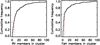 |
Fig. 1. Left panel: cumulative number of RVs members in 295 OCs. About 59% of the clusters have more than five RVs members. Right panel: cumulative number of [Fe/H] members in 220 OCs. About 38% clusters have more than five [Fe/H] members. |
It is not suitable to simply use the mean RVs of members as the overall RVs of an open cluster. This is because the mean RVs is easy to be contaminated by misidentified member stars (in fact, they are field stars with different RVs) or member stars with large RVs measurement uncertainties (e.g., stars of early or late type, or stars with low S/N). The mean RVs of members have large uncertainties and lead to unpredictable offsets, especially for clusters with only a few RVs members.
To solve this problem and derive a reliable average RVs for OCs, we carefully checked the RVs distribution histogram of each open cluster, and for those with sufficient RVs data we used a Gaussian profile to fit the RVs distribution of member stars. Outliers were excluded in the Gaussian fitting process. For each cluster, the μ and σ of the Gaussian function was used as the average RVs and corresponding uncertainty. Figure 2 shows a few examples of the RVs fitting results. In our sample, clusters that have the average RVs estimation derived by the Gaussian fitting process are marked as the high-quality samples with the RV_flag labeled “Y” in the catalog (see Table 1). On the other hand, for clusters with a small number of RVs members or with large dispersion in RVs distribution, we simply provided mean RVs and standard deviations as their overall RVs and uncertainties, respectively.
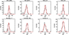 |
Fig. 2. RVs distribution and fitting profile for each open cluster. The complete list of fitting results is available along with the catalog data (see Sect. 4). |
Description of the open cluster properties catalog.
2.3. Metallicities
The fifth data release of LAMOST (DR5) provides a stellar parameter catalog of 5.3 million spectra (Luo et al. 2015). Following the determination process of the overall RVs of OCs, we first cross-matched cluster members of CG18 with the stellar parameter catalog in LAMOST. Then we selected stars with membership probabilities higher than 0.5 and with available [Fe/H] measurements; 3024 stars in 220 clusters were selected for metallicity estimation.
Using members with [Fe/H] measurement, we plotted the metallicity distribution histogram and performed Gaussian fitting for each open cluster. As we did in the RVs estimation, outliers that have very different metallicity values were excluded by visual inspection. A few examples of the fitting results are presented in Fig. 3, while the μ and σ of Gaussian function are used as the average metallicity and corresponding uncertainty, respectively. For the rest of OCs whose metallicity distribution cannot be fitted by the Gaussian function, their overall metallicities and uncertainties are set as the mean [Fe/H] and standard deviations, respectively.
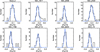 |
Fig. 3. [Fe/H] metallicity distribution and fitting profile for each open cluster. The complete list of fitting results is available along with the catalog data (see Sect. 4). |
In order to further understand the internal consistency and parameter independence of [Fe/H] metallicity of LAMOST DR5, we studied the [Fe/H] distribution as a function of Teff and Log g. Using the same clusters in Fig. 3 as examples, Figs. 4 and 5 show [Fe/H] versus Teff and [Fe/H] versus Log g results, respectively. Although there are a few outliers or stars with large [Fe/H] measurement errors, there is no apparent degeneracy between [Fe/H] and other parameters, and the fitting results (dashed line) properly represent the overall metallicity of these clusters.
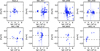 |
Fig. 4. [Fe/H] metallicity distribution as a function of temperature (Teff) for each open cluster. The dashed line represents the overall [Fe/H] metallicity derived by Gaussian fitting in Fig. 3. |
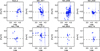 |
Fig. 5. [Fe/H] metallicity distribution as a function of surface gravity (Log g) for each open cluster. The dashed line represents the overall [Fe/H] metallicity derived by Gaussian fitting in Fig. 3. |
2.4. Ages
In order to provide the age parameter of our sample clusters, we utilized literature results from Dias et al. (2002), Kharchenko et al. (2012), and Bossini et al. (2019) to perform the isochrone fitting and visually determine best fitting result of the age, distance, and reddening parameters. Since membership probabilities provided by CG18 are more reliable than those of previous works, member stars used for isochrone fitting come from CG18 with probability greater than 0.5. We only provide literature parameters whose isochrone is consistent with the distribution of cluster members in the color-magnitude diagram. In other words, if the age parameter of a cluster in our catalog is zero, that means none of the literature parameters can meet the distribution of cluster members properly. Figure 6 presents a few examples of the isochrone fitting results.
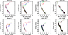 |
Fig. 6. Examples of member distribution in color-magnitude diagram. Colors represent the isochrone parameters provided by different literature sources: Dias et al. (2002) in green, Kharchenko et al. (2012) in blue, and Bossini et al. (2019) in red. The complete list of fitting results is available along with the catalog data (see Sect. 4). |
2.5. Kinematic parameters
We calculated the Galactocentric cartesian coordinates (X, Y, Z) and velocities (U, V, W) of 295 OCs by using formulas in Johnson & Soderblom (1987). The celestial coordinates, distance, and proper motions of each cluster are from CG18, while the RVs is determined from the LAMOST DR5 (see Sect. 2.2). We adopt the solar position and its circular rotation velocity as R0 = −8.34 kpc and Θ0 = 240 km s−1, respectively (Reid et al. 2014). In order to correct for the solar motion in the local standard of rest, we adopt the solar peculiar velocity as (U⊙, V⊙, W⊙) = (11.1, 12.4, 7.25) km s−1 (Schönrich et al. 2010).
Based on the astrometry parameters from Gaia DR2 and LAMOST DR5, we also calculated the orbital parameters of 295 OCs making use of galpy2 (Bovy 2015). The orbital parameters are listed in Table 1, including apogalactic (Rap) and perigalactic (Rperi) distances from the Galactic centre, orbital eccentricity (e), and the maximum vertical distance above the Galactic plane (Zmax).
Figure 7 shows the distribution of derived spatial and kinematic parameters (blue dots). In particular, we use the color red to represent 109 clusters that have RVs estimations with high quality (RV_flag labeled “Y”; see Sect. 2.2). The kinematic parameters, specifically orbital parameters of these clusters (red dots) are more reliable than the others. The Galactocentric spatial distribution of the 295 OCs in our catalog are shown in the top panels. We find that most of clusters are located on the Galactic anti-center; this is because a large number of LAMOST observational fields are focused on this region. The Galactocentric velocities of OCs are shown in middle panels. In particular, we exclude six OCs from the velocity and the orbital parameter distribution (bottom panels) since their unreliable radial velocities led to outliers of kinematic parameters. In the bottom panels, the distribution of orbital parameters show that most of the OCs have approximate circular motions and small distances to the Galactic plane. Specifically, the kinematic distribution diagrams clearly illustrate that most of the OCs in our catalog are kinematically typical thin disks.
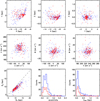 |
Fig. 7. Distribution of derived spatial and kinematic parameters. The blue dots are the 295 OCs with RVs estimations. The red dots are 109 OCs that have RVs measurements with high quality. The distribution of clusters illustrate that they are located on the Galactic plane and have kinematics typical of the thin disk. |
2.6. Comparison to other works
To verify the reliability and accuracy of the cluster properties derived by LAMOST DR5, we employed clusters in common between our catalog and other literature catalogs that have high-resolution observations.
2.6.1. Verifying radial velocities
As we describe in Sect. 1, Gaia DR2 also include accurate radial velocities for 7.2 million stars, which were provided by the high-resolution slitless spectrograph (R = 11 500). SC18 published mean RVs for 861 star clusters using spectral results from the Gaia DR2. We used our catalog to cross-match with SC18 and obtained 218 common clusters. In order to use reliable clusters in SC18 as reference, our comparison only includes 83 common clusters defined as high-quality clusters (see details in SC18). In addition, we also exclude 12 common clusters since their mean RVs in our catalog are unreliable (uncertainty greater than 20 km s−1). Finally, the number of common clusters used for comparison is 71.
Figure 8 (upper panel) shows the RVs differences between SC18 and our catalog for OCs in common. The average offset of RVs is −5.1 km s−1 with a scatter of 6.4 km s−1. In general, this result shows good agreement with Gaia. The scatter is mainly caused by the RVs uncertainties of LAMOST spectra R = 1800, (σ ∼ 5 km s−1), and the number of LAMOST stars in a cluster used for mean RVs estimation (red dots have less scatter than violet dots).
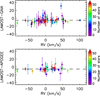 |
Fig. 8. Upper panel: RVs differences for 71 common clusters between SC18 and our catalog. Bottom panel: RVs differences for 36 common clusters between DJ20 and our catalog. The solid circles and their corresponding error bars represent the mean RVs and dispersion of each cluster in our catalog, respectively. The color of the data points represents the number of stars used to estimate the average in our catalog. As a comparison of the results of overall RVs of OCs, the average difference for LAMOST-Gaia and LAMOST-APOGEE is −5.1 ± 6.4 km s−1 and −5.5 ± 5.4 km s−1, respectively. |
In particular, we note that there is an outlier (blue dot in the upper panel of Fig. 8) with a discrepant RVs greater than 20 km s−1: FSR_0904. After carefully checking the RVs data of two catalogs, we find there are three stars for the mean RVs estimation for SC18 and 20 for our catalog. Figure 9 shows the spatial distribution and color-magnitude distribution of member stars which were used by two works. At least for this cluster, although the scatter of mean RVs in our catalog (7.2 km s−1) is greater than in SC18 (2.66 km s−1), it is more reliable for the mean RVs provided by our catalog since our stars are mainly distributed on the cluster center and follow the cluster main sequence.
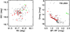 |
Fig. 9. Spatial distribution (left panel) and color-magnitude distribution (right panel) of member stars of FSR_0904. Black dots are cluster members in CG18. Green and red dots are member stars used for RVs estimation in SC18 and our catalog, respectively. It is clear that our RVs value of this cluster is more reliable since most of our stars are more likely to be cluster members. |
In addition, we used our catalog and the APOGEE catalog (Donor et al. 2020, hereafter DJ20) to perform the comparison of mean RVs and mean [Fe/H] abundance. There are 128 OCs published by DJ20, including mean RVs and mean abundances from the APOGEE DR16. After cross-matching with two catalogs, our sample includes 48 OCs in common with DJ20. Six OCs were further excluded since their “qual” in DJ20 are flagged as “0” or “potentially unreliable”.
For the comparison of mean RVs difference with the APOGEE catalog, 36 common clusters, whose RVs uncertainty in our catalog are smaller than 20 km s−1, are plotted in the bottom panel of Fig. 8. The average offset of RVs is −5.5 km s−1 with a scatter of 5.4 km s−1. Similarly to the Gaia result, our mean RVs results of clusters are also consistent with the APOGEE catalog, especially for clusters which have more stars to estimate the mean values.
We note that there are similar RVs offsets between our catalog and literature catalogs (SC18 and DJ20) of around −5 km s−1. In order to understand the origin and amount of this offset in LAMOST, we perform a general cross-match of stars between LAMOST DR5 and other spectroscopic catalogs (GALAH DR2, APOGEE DR16, and Gaia DR2). Table 2 shows the results of RVs difference for common stars whose S/N in LAMOST are greater than 10. Here we list the median RVs offset, the mean RVs offset, standard deviation of RVs difference, and the number of common stars used for calculation. The similar comparison results of general stars and OCs show that the RVs difference are mainly from the measurement of LAMOST spectra. In addition, we study the RVs offset as a function of stellar atmospheric parameters and find that the RVs offset is almost constant over all the parameter space. The result of RVs differences is also consistent with the conclusion of LAMOST LSP3 parameters analysis (Xiang et al. 2015).
Difference in RVs for general common stars between LAMOST DR5 and other spectroscopic catalogs.
2.6.2. Verifying metallicities
We compared the [Fe/H] metallicity between our catalog and DJ20. In Fig. 10, there are 38 common clusters whose [Fe/H] uncertainty values in our catalog are not zero and we find a mean offset in [Fe/H] of −0.02 dex and a scatter of 0.10 dex. We note that all discrepant values are from clusters with the lower number of stars for estimation. Excluding clusters whose number of stars for estimation are less than 10, our result shows good agreement with APOGEE result.
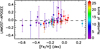 |
Fig. 10. [Fe/H] differences for 38 common clusters between DJ20 and our catalog. The solid circles and their corresponding error bars represent the mean [Fe/H] and dispersion of each cluster in our catalog, respectively. As a comparison result of overall [Fe/H] of OCs, the average difference is −0.02 ± 0.10 dex. |
Furthermore, we note that the offset shows a tiny gradient along the metallicity in Fig. 10. In order to study the origin of this trend, we compare the metallicity difference of common stars between LAMOST DR5 and other spectroscopic catalogs (GALAH DR2 and APOGEE DR16). To reduce the effect of stars with low S/N, for comparison we only select common stars whose LAMOST S/N are greater than 10. Table 3 list the comparison results of metallicity offset and dispersion. The overall small offsets and dispersion indicate the reliability of metallicity measurement in LAMOST DR5 since they are in good agreement with high-resolution spectroscopic results.
Differences in [Fe/H] for general common stars between LAMOST DR5 and other spectroscopic catalogs.
In Fig. 11, we plot the stellar [Fe/H] metallicity difference between LAMOST DR5 and GALAH DR2 and APOGEE DR16. We note that the [Fe/H] difference of dwarfs between LAMOST and APOGEE shows a positive gradient along the metallicity, which also indicates that the trend in Fig. 10 may come from the measurement difference of dwarfs between the two catalogs.
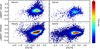 |
Fig. 11. [Fe/H] metallicity differences for common stars as a function of LAMOST metallicity. Giants and dwarfs are separated by adopting the criteria of log g < 3 and log g > 3, respectively. |
3. Abundance analysis
3.1. Radial metallicity gradient
The radial metallicity gradient in the Galactic disk plays an important role in studying the chemical formation and evolution of the Galaxy. In addition to stars or planetary nebulae (PNe) (e.g., Luck & Lambert 2011; Bergemann et al. 2014), OCs are ideal tracers of the radial metallicity gradient study; since they have a wide span of ages and distances, their coeval member stars have small metallicity dispersion. From open cluster sample in previous works, the radial metallicity gradients range from −0.052 to −0.063 dex kpc−1 within 12 kpc (Chen et al. 2003; Wu et al. 2009; Pancino et al. 2010; Reddy et al. 2016; Netopil et al. 2016).
In our sample, most of OCs are younger than 3 Gyr. We use these clusters to fit the average radial metallicity gradient of young component in the Galactic disk. The upper panel in Fig. 12 shows the metallicity gradient in the Galactocentric distance range RGC = 7−15 kpc, with a linear fit to the whole range. Although the radial metallicity gradient of −0.053 ± 0.004 dex kpc−1 in the radial range 7−15 kpc is consistent with the previous works (see Table 4 for more details and comparison), the Pearson correlation coefficient of −0.33 indicates a weak correlation for overall radial metallicity gradient of all clusters, which may be caused by the mixture of OCs with different populations.
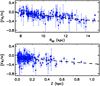 |
Fig. 12. Radial (upper panel) and vertical (bottom panel) metallicity gradient of young OCs. The slope of gradients is −0.053 ± 0.004 dex kpc−1 and −0.252 ± 0.039 dex kpc−1, respectively. |
In order to constrain the Galactic chemo-dynamical model, the study of gradient evolution in the Galactic disk is important (Carraro et al. 1998; Chen et al. 2003; Yong et al. 2012). Figure 13 shows the radial metallicity gradients in different age bins. Since we have a sufficient number of clusters in different age bins, we can perform the analysis of gradient evolution. We separate our samples into five age bins, including a very young age bin (< 0.1 Gyr), from young to intermediate age bins, (0.1−0.5 Gyr, 0.5−1.0 Gyr, 1.0−2.0 Gyr), and old age bin (> 2.0 Gyr). Table 5 show the Pearson correlation coefficient of radial metallicity gradients in different age bins. After separating clusters with age bins, the Pearson correlation coefficient shows that the correlation of metallicity gradients in different age bins is stronger than the correlation of overall metallicity gradient, which also indicates the higher reliability of radial metallicity gradients in different age bins. The gradient trend with median age of each subsample is shown in the left panel of Fig. 14. Ignoring the very young sample, the other four age samples display a mild flat trend of radial metallicity gradient with time. For clusters with age greater than 0.1 Gyr (most of them less than 4 Gyr), the steeper gradient of older population is consistent with previous studies (e.g., Carraro et al. 1998; Friel et al. 2002; Donor et al. 2020). The time-flattening tendency may be explained by the common influence of radial migration (Netopil et al. 2016; Anders et al. 2017) and chemical evolution in the Galactic disk (Tosi 2000; Chang et al. 2002; Jacobson et al. 2016).
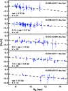 |
Fig. 13. Radial metallicity gradients in different age bins. Dashed lines are linear least-squares approximations in one-dimension with [Fe/H] errors. |
Summary of reported radial metallicity gradients using OCs as tracers.
However, we note that there is a steep gradient for very young samples (< 0.1 Gyr) that is not consistent with previous results (Carrera & Pancino 2011; Spina et al. 2017) and the corresponding explanation (Baratella et al. 2020). Although there is no convincing explanation for this reverse trend, this result is not contradictory to the chemo-dynamical simulation of Minchev et al. (2013, 2014, MCM). In the MCM model, radial migration is expected to flatten the chemical gradients for ages > 1 Gyr, while it also predicts an almost unchanged gradient for the very young population. Since there is no process that has a significant impact on the gradient of very young population, their steep gradient partly represent the current chemical gradient in the Galactic disk (RGC ∼ 8−12 kpc).
In particular, it is noteworthy that the cluster NGC 6791 is included in our initial sample. As many previous works noted, this cluster is very metal-rich and fairly old (Carraro & Chiosi 1994; Tofflemire et al. 2014; Donor et al. 2018), and is believed to have migrated to its current location (Linden et al. 2017). In order to reduce the influence of outliers on gradients, we excluded NGC 6791 from our cluster sample, and then performed the radial and vertical gradient analysis shown in Figs. 12–15.
3.2. Vertical metallicity gradient
The vertical metallicity gradient is another important clue to constrain the formation history of the Galactic disk, while its existence among old OCs was controversial (Friel 1995; Piatti et al. 1995). The bottom panel in Fig. 12 show the vertical metallicity gradient of our clusters within 1 kpc distance from the Galactic mid-plane. The resulting slope is −0.252 ± 0.039 dex kpc−1, which is in good agreement with previous results (e.g., Carraro et al. 1998; Chen et al. 2003).
As Carraro et al. (1998) pointed out, the cluster sample that they used to derive the vertical gradient is significantly biased because of the tidal disruption, which is more effective when closer to the Galactic mid-plane. In order to disentangle the effect of age dependence, we plot the vertical gradients in different age bins in Fig. 15, and the gradient trend along the median age of each age sample in Fig. 14 (right panel), while age bins are the same as in radial gradient analysis. The Pearson correlation coefficients of vertical metallicity distribution with different age bins are presented in Table 5, which show weak correlation or even no correlation. It is worth noting that the vertical distribution of OCs is affected by the different scale-heights of different age populations (Ng et al. 1996). For very young samples (< 0.1 Gyr), the positive gradient may be caused by the small scale-height, which also leads a large dispersion of the trend. For old samples (> 2 Gyr), we suppose the positive gradient is the result of both migration and tidal disruption. Therefore, this suggests that OCs with intermediate ages provide a more reliable trend of vertical metallicity gradient than other age populations.
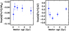 |
Fig. 14. Radial (left panel) and vertical (right panel) metallicity gradient trends along the median age of each age bin. |
Pearson correlation coefficients of radial and vertical metallicity gradients in different age bins.
3.3. Age-metallicity relation
The age-metallicity relation (AMR) is a useful clue for understanding the history of metal enrichment of the disk; it provides an important constraint on the chemical evolution models. During the past two decades, many works have been focused on this study, either using nearby stars (Feltzing et al. 2001; Carraro et al. 1998; Edvardsson et al. 1993) or OCs with multiple ages (Netopil et al. 2016; Chen et al. 2003; Carraro et al. 1998). In general, the observational data shows the evidence of decreasing metallicity with increasing age for both tracers, which indicate in principle the metal-enrichment in the interstellar medium (ISM) during the chemical evolution of the Galaxy.
Compared with the nearby stars, the OCs have a great advantage in identifying the AMR since their metallicities and ages can be more reliably determined. However, even based on the OCs, the existence of AMR on the disk is not significant (Magrini et al. 2009; Carraro & Chiosi 1994; Cameron 1985). For some studies, only a mild decrease in the metal content of clusters with age is found (Netopil et al. 2016; Pancino et al. 2010; Chen et al. 2003).
Figure 16 shows the age-metallicity relation of OCs in our catalog. Ages were determined by visual inspection through the best fitting isochrone in the color-magnitude diagram (see Sect. 2.4). To remove the effect of the spatial variation of the metallicity due to the radial metallicity gradients, we build up an AMR in which we correct our [Fe/H] with the following relation [Fe/H]corr = [Fe/H]−0.053 (R⊙ − R) (kpc). After excluding three old OCs as outliers, we perform the linear fitting of OCs in our sample. The metallicity decreases with 0.022 ± 0.008 dex Gyr−1 for OCs within 6 Gyr. The Pearson correlation coefficients of −0.28 also indicate the weak correlation of AMR, which is consistent with the mild decrease relation in previous works (e.g., Netopil et al. 2016; Pancino et al. 2010; Chen et al. 2003).
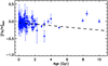 |
Fig. 16. Age-metallicity relation of OCs. In our sample, the slope for OCs with age < 6 Gyr is −0.022 ± 0.008 dex Gyr−1. Three outliers are shown as triangles, and are excluded from the linear fitting procedure. |
We note that there are three very old but metal-rich OCs in our sample (triangles in Fig. 16), with age of 8 Gyr or older. One of the possible explanations for the origin of these OCs is the infalling or merger events within the time of 3−5 Gyr (Carraro et al. 1998). For OCs with age > 8 Gyr, it is suggested that they might be related by the formation of the triaxial bar structure (Ng et al. 1996) and further migrated to the current position.
4. Description of the catalog
We provide two catalogs3 in this paper: one for the properties of 295 OCs and the other for spectroscopic parameters of 8811 member stars.
Table 1 describes the catalog of open cluster properties. Columns 2−8 list astrometic parameters of OCs provided by CG18, including the coordinates, mean proper motions, and distances, which were mainly based on the Gaia solution. Columns 9−16 list the measurement results of RVs and metallicity by LAMOST DR5. Columns 17−34 list the derived kinematic and orbital parameters of OCs. Columns 35−38 list the parameters by the isochrone fit results in the literature, including age, distance, and reddening.
Table 6 describes the spectroscopic catalog of cluster members, including the LAMOST spectra information (Cols. 1−7), the derived stellar fundamental parameters by the LAMOST spectra (Cols. 8−17), the astrometric and photometric parameters in Gaia DR2 (Cols. 18−26), and the membership probability in CG18 (Col. 27).
Description of the spectroscopic catalog of cluster members.
5. Summary
We used the cluster members identified by CG18 to cross-match with the LAMOST spectroscopic catalog. A total of 8811 member stars with spectrum data were provided. Using the spectral information of cluster members, we also provided average RVs of 295 OCs and metallicity of 220 OCs. Considering the accurate observed data of tangential velocity provided by Gaia DR2 and RVs provided by LAMOST DR5, we further derived the 6D phase positions and orbital parameters of 295 OCs. The kinematic results shows that most of the OCs in our catalog are located on the thin disk and have approximate circular motions. In addition, referring to the literature results of using isochrone fitting method, we estimated the age, distance, and reddening of our sample of OCs.
As an value-added catalog in LAMOST DR5, the provided list of cluster members make a correlation between the LAMOST spectra and the cluster overall properties, especially for stellar age, reddening, and the distance module. Compared with the spectra of field stars, the LAMOST spectra of member stars are valuable sources to perform the detail study of stellar physics or to calibrate the stellar fundamental parameters since the cluster can provide statistical information for these members with higher precision.
Furthermore, using the OCs as tracers, we make use of their metallicities to study the radial metallicity gradient and the age-metallicity relation. The derived radial metallicity gradient for young clusters is −0.053 ± 0.004 dex kpc−1 within the radial range of 7−15 kpc, which is consistent with previous works. After excluding seven old, but metal-rich OCs, we derived an AMR as −0.022 ± 0.008 dex Gyr−1 for young clusters, which follow the tendency that younger clusters have higher metallicities as a consequence of the more enriched ISM from which they formed (Magrini et al. 2009). On the other hand, considering that the increase in metallicity of the disk has been mild during the past 5 Gyr (Chen et al. 2003), which is indeed in agreement with our findings of a small increase in the youngest clusters, the nature of the AMR of OCs needs further investigations.
The catalogs can be downloaded via http://dr5.lamost.org/doc/vac and via the CDS.
Acknowledgments
We are very grateful to the referee for helpful suggestions, as well as the correction for some language issues, which have improved the paper significantly. This work supported by National Key R&D Program of China No. 2019YFA0405501. The authors acknowledges the National Natural Science Foundation of China (NSFC) under grants U1731129 (PI: Zhong), 11373054 and 11661161016 (PI: Chen) and Guoshoujing Telescope (the Large Sky Area Multi-Object Fiber Spectroscopic Telescope LAMOST) is a National Major Scientific Project built by the Chinese Academy of Sciences. Funding for the project has been provided by the National Development and Reform Commission. LAMOST is operated and managed by the National Astronomical Observatories, Chinese Academy of Sciences. This work has made use of data from the European Space Agency (ESA) mission Gaia (https://www.cosmos.esa.int/gaia), processed by the Gaia Data Processing and Analysis Consortium (DPAC, https://www.cosmos.esa.int/web/gaia/dpac/consortium). Funding for the DPAC has been provided by national institutions, in particular the institutions participating in the Gaia Multilateral Agreement.
References
- Ahumada, R., Allende Prieto, C., Almeida, A., et al. 2020, ApJS, 249, 3 [CrossRef] [Google Scholar]
- Anders, F., Chiappini, C., Minchev, I., et al. 2017, A&A, 600, A70 [NASA ADS] [CrossRef] [EDP Sciences] [Google Scholar]
- Baratella, M., D’Orazi, V., Carraro, G., et al. 2020, A&A, 634, A34 [CrossRef] [EDP Sciences] [Google Scholar]
- Bergemann, M., Ruchti, G. R., Serenelli, A., et al. 2014, A&A, 565, A89 [NASA ADS] [CrossRef] [EDP Sciences] [Google Scholar]
- Bragaglia, A., Sestito, P., Villanova, S., et al. 2008, A&A, 480, 79 [NASA ADS] [CrossRef] [EDP Sciences] [Google Scholar]
- Buder, S., Asplund, M., Duong, L., et al. 2018, MNRAS, 478, 4513 [NASA ADS] [CrossRef] [Google Scholar]
- Bobylev, V. V., & Bajkova, A. T. 2019, Astron. Lett., 45, 208 [CrossRef] [Google Scholar]
- Bossini, D., Vallenari, A., Bragaglia, A., et al. 2019, A&A, 623, A108 [NASA ADS] [CrossRef] [EDP Sciences] [Google Scholar]
- Bovy, J. 2015, ApJS, 216, 29 [NASA ADS] [CrossRef] [Google Scholar]
- Cameron, L. M. 1985, A&A, 147, 47 [NASA ADS] [Google Scholar]
- Carraro, G., & Chiosi, C. 1994, A&A, 287, 761 [NASA ADS] [Google Scholar]
- Carraro, G., Ng, Y. K., & Portinari, L. 1998, MNRAS, 296, 1045 [NASA ADS] [CrossRef] [Google Scholar]
- Carrera, R., & Pancino, E. 2011, A&A, 535, A30 [NASA ADS] [CrossRef] [EDP Sciences] [Google Scholar]
- Cantat-Gaudin, T., Jordi, C., Vallenari, A., et al. 2018, A&A, 618, A93 [NASA ADS] [CrossRef] [EDP Sciences] [Google Scholar]
- Cantat-Gaudin, T., Krone-Martins, A., Sedaghat, N., et al. 2019, A&A, 624, A126 [NASA ADS] [CrossRef] [EDP Sciences] [Google Scholar]
- Castro-Ginard, A., Jordi, C., Luri, X., et al. 2018, A&A, 618, A59 [NASA ADS] [CrossRef] [EDP Sciences] [Google Scholar]
- Chang, R.-X., Shu, C.-G., & Hou, J.-L. 2002, Chin. J. Astron. Astrophys., 2, 226 [CrossRef] [Google Scholar]
- Chen, L., Hou, J. L., & Wang, J. J. 2003, AJ, 125, 1397 [NASA ADS] [CrossRef] [Google Scholar]
- Cui, X. Q., Zhao, Y. H., Chu, Y. Q., et al. 2012, Res. Astron. Astrophys., 12, 1197 [NASA ADS] [CrossRef] [Google Scholar]
- Cropper, M., Katz, D., Sartoretti, P., et al. 2018, A&A, 616, A5 [NASA ADS] [CrossRef] [EDP Sciences] [Google Scholar]
- Donor, J., Frinchaboy, P. M., Cunha, K., et al. 2018, AJ, 156, 142 [NASA ADS] [CrossRef] [Google Scholar]
- Donor, J., Frinchaboy, P. M., Cunha, K., et al. 2020, AJ, 159, 199 [Google Scholar]
- Dias, W. S., Alessi, B. S., Moitinho, A., & Lépine, J. R. D. 2002, A&A, 389, 871 [NASA ADS] [CrossRef] [EDP Sciences] [Google Scholar]
- Edvardsson, B., Andersen, J., Gustafsson, B., et al. 1993, A&A, 500, 391 [NASA ADS] [Google Scholar]
- Feltzing, S., Holmberg, J., & Hurley, J. R. 2001, A&A, 377, 911 [NASA ADS] [CrossRef] [EDP Sciences] [Google Scholar]
- Ferreira, F. A., Santos, J. F. C., Corradi, W. J. B., Maia, F. F. S., & Angelo, M. S. 2019, MNRAS, 483, 5508 [NASA ADS] [CrossRef] [Google Scholar]
- Friel, E. D. 1995, ARA&A, 33, 381 [NASA ADS] [CrossRef] [Google Scholar]
- Friel, E. D., & Janes, K. A. 1993, A&A, 267, 75 [NASA ADS] [Google Scholar]
- Friel, E. D., Janes, K. A., Tavarez, M., et al. 2002, AJ, 124, 2693 [NASA ADS] [CrossRef] [Google Scholar]
- Friel, E. D., Jacobson, H. R., & Pilachowski, C. A. 2010, AJ, 139, 1942 [NASA ADS] [CrossRef] [Google Scholar]
- Gaia Collaboration (Brown, A. G. A., et al.) 2018, A&A, 616, A1 [NASA ADS] [CrossRef] [EDP Sciences] [Google Scholar]
- Jacobson, H. R., Friel, E. D., Jílková, L., et al. 2016, A&A, 591, A37 [NASA ADS] [CrossRef] [EDP Sciences] [Google Scholar]
- Janes, K. A. 1979, ApJS, 39, 135 [NASA ADS] [CrossRef] [Google Scholar]
- Johnson, D. R. H., & Soderblom, D. R. 1987, AJ, 93, 864 [NASA ADS] [CrossRef] [Google Scholar]
- Kharchenko, N. V., Piskunov, A. E., Schilbach, E., Röser, S., & Scholz, R.-D. 2012, A&A, 543, A156 [NASA ADS] [CrossRef] [EDP Sciences] [Google Scholar]
- Kharchenko, N. V., Piskunov, A. E., Schilbach, E., Röser, S., & Scholz, R.-D. 2013, A&A, 558, A53 [NASA ADS] [CrossRef] [EDP Sciences] [Google Scholar]
- Krone-Martins, A., & Moitinho, A. 2014, A&A, 561, A57 [NASA ADS] [CrossRef] [EDP Sciences] [Google Scholar]
- Linden, S. T., Pryal, M., Hayes, C. R., et al. 2017, ApJ, 842, 49 [NASA ADS] [CrossRef] [Google Scholar]
- Lindegren, L., Hernández, J., Bombrun, A., et al. 2018, A&A, 616, A2 [NASA ADS] [CrossRef] [EDP Sciences] [Google Scholar]
- Luo, A.-L., Zhang, H.-T., Zhao, Y.-H., et al. 2012, Res. Astron. Astrophys., 12, 1243 [NASA ADS] [CrossRef] [Google Scholar]
- Luo, A.-L., Zhao, Y.-H., Zhao, G., et al. 2015, Res. Astron. Astrophys., 15, 1095 [NASA ADS] [CrossRef] [Google Scholar]
- Luck, R. E., & Lambert, D. L. 2011, AJ, 142, 136 [Google Scholar]
- Magrini, L., Sestito, P., Randich, S., et al. 2009, A&A, 494, 95 [NASA ADS] [CrossRef] [EDP Sciences] [Google Scholar]
- Meingast, S., & Alves, J. 2019, A&A, 621, L3 [NASA ADS] [CrossRef] [EDP Sciences] [Google Scholar]
- Minchev, I., Chiappini, C., & Martig, M. 2013, A&A, 558, A9 [NASA ADS] [CrossRef] [EDP Sciences] [Google Scholar]
- Minchev, I., Chiappini, C., & Martig, M. 2014, A&A, 572, A92 [NASA ADS] [CrossRef] [EDP Sciences] [Google Scholar]
- Netopil, M., Paunzen, E., Heiter, U., & Soubiran, C. 2016, A&A, 585, A150 [NASA ADS] [CrossRef] [EDP Sciences] [Google Scholar]
- Ng, Y. K., Bertelli, G., Chiosi, C., et al. 1996, A&A, 310, 771 [Google Scholar]
- Pancino, E., Carrera, R., Rossetti, E., et al. 2010, A&A, 511, A56 [NASA ADS] [CrossRef] [EDP Sciences] [Google Scholar]
- Piatti, A. E., Claria, J. J., & Abadi, M. G. 1995, AJ, 110, 2813 [NASA ADS] [CrossRef] [Google Scholar]
- Reddy, A. B. S., Lambert, D. L., & Giridhar, S. 2016, MNRAS, 463, 4366 [NASA ADS] [CrossRef] [Google Scholar]
- Reid, M. J., Menten, K. M., Brunthaler, A., et al. 2014, ApJ, 783, 130 [Google Scholar]
- Röser, S., Schilbach, E., & Goldman, B. 2019, A&A, 621, L2 [NASA ADS] [CrossRef] [EDP Sciences] [Google Scholar]
- Sestito, P., Bragaglia, A., Randich, S., et al. 2008, A&A, 488, 943 [NASA ADS] [CrossRef] [EDP Sciences] [Google Scholar]
- Schönrich, R., Binney, J., & Dehnen, W. 2010, MNRAS, 403, 1829 [NASA ADS] [CrossRef] [Google Scholar]
- Soubiran, C., Cantat-Gaudin, T., Romero-Gómez, M., et al. 2018, A&A, 619, A155 [NASA ADS] [CrossRef] [EDP Sciences] [Google Scholar]
- Spina, L., Randich, S., Magrini, L., et al. 2017, A&A, 601, A70 [NASA ADS] [CrossRef] [EDP Sciences] [Google Scholar]
- Tofflemire, B. M., Gosnell, N. M., Mathieu, R. D., et al. 2014, AJ, 148, 61 [NASA ADS] [CrossRef] [Google Scholar]
- Tosi, M. 2000, Astrophys. Space Sci. Lib., 505, 334 [Google Scholar]
- Wu, Z.-Y., Zhou, X., Ma, J., et al. 2009, MNRAS, 399, 2146 [NASA ADS] [CrossRef] [Google Scholar]
- Xiang, M. S., Liu, X. W., Yuan, H. B., et al. 2015, MNRAS, 448, 822 [NASA ADS] [CrossRef] [Google Scholar]
- Yong, D., Carney, B. W., & Friel, E. D. 2012, AJ, 144, 95 [NASA ADS] [CrossRef] [Google Scholar]
- Zhao, G., Zhao, Y.-H., Chu, Y.-Q., et al. 2012, Res. Astron. Astrophys., 12, 723F [CrossRef] [Google Scholar]
- Zhong, J., Chen, L., Kouwenhoven, M. B. N., et al. 2019, A&A, 624, A34 [CrossRef] [EDP Sciences] [Google Scholar]
All Tables
Difference in RVs for general common stars between LAMOST DR5 and other spectroscopic catalogs.
Differences in [Fe/H] for general common stars between LAMOST DR5 and other spectroscopic catalogs.
Pearson correlation coefficients of radial and vertical metallicity gradients in different age bins.
All Figures
|
Fig. 1. Left panel: cumulative number of RVs members in 295 OCs. About 59% of the clusters have more than five RVs members. Right panel: cumulative number of [Fe/H] members in 220 OCs. About 38% clusters have more than five [Fe/H] members. |
| In the text | |
|
Fig. 2. RVs distribution and fitting profile for each open cluster. The complete list of fitting results is available along with the catalog data (see Sect. 4). |
| In the text | |
|
Fig. 3. [Fe/H] metallicity distribution and fitting profile for each open cluster. The complete list of fitting results is available along with the catalog data (see Sect. 4). |
| In the text | |
|
Fig. 4. [Fe/H] metallicity distribution as a function of temperature (Teff) for each open cluster. The dashed line represents the overall [Fe/H] metallicity derived by Gaussian fitting in Fig. 3. |
| In the text | |
|
Fig. 5. [Fe/H] metallicity distribution as a function of surface gravity (Log g) for each open cluster. The dashed line represents the overall [Fe/H] metallicity derived by Gaussian fitting in Fig. 3. |
| In the text | |
|
Fig. 6. Examples of member distribution in color-magnitude diagram. Colors represent the isochrone parameters provided by different literature sources: Dias et al. (2002) in green, Kharchenko et al. (2012) in blue, and Bossini et al. (2019) in red. The complete list of fitting results is available along with the catalog data (see Sect. 4). |
| In the text | |
|
Fig. 7. Distribution of derived spatial and kinematic parameters. The blue dots are the 295 OCs with RVs estimations. The red dots are 109 OCs that have RVs measurements with high quality. The distribution of clusters illustrate that they are located on the Galactic plane and have kinematics typical of the thin disk. |
| In the text | |
|
Fig. 8. Upper panel: RVs differences for 71 common clusters between SC18 and our catalog. Bottom panel: RVs differences for 36 common clusters between DJ20 and our catalog. The solid circles and their corresponding error bars represent the mean RVs and dispersion of each cluster in our catalog, respectively. The color of the data points represents the number of stars used to estimate the average in our catalog. As a comparison of the results of overall RVs of OCs, the average difference for LAMOST-Gaia and LAMOST-APOGEE is −5.1 ± 6.4 km s−1 and −5.5 ± 5.4 km s−1, respectively. |
| In the text | |
|
Fig. 9. Spatial distribution (left panel) and color-magnitude distribution (right panel) of member stars of FSR_0904. Black dots are cluster members in CG18. Green and red dots are member stars used for RVs estimation in SC18 and our catalog, respectively. It is clear that our RVs value of this cluster is more reliable since most of our stars are more likely to be cluster members. |
| In the text | |
|
Fig. 10. [Fe/H] differences for 38 common clusters between DJ20 and our catalog. The solid circles and their corresponding error bars represent the mean [Fe/H] and dispersion of each cluster in our catalog, respectively. As a comparison result of overall [Fe/H] of OCs, the average difference is −0.02 ± 0.10 dex. |
| In the text | |
|
Fig. 11. [Fe/H] metallicity differences for common stars as a function of LAMOST metallicity. Giants and dwarfs are separated by adopting the criteria of log g < 3 and log g > 3, respectively. |
| In the text | |
|
Fig. 12. Radial (upper panel) and vertical (bottom panel) metallicity gradient of young OCs. The slope of gradients is −0.053 ± 0.004 dex kpc−1 and −0.252 ± 0.039 dex kpc−1, respectively. |
| In the text | |
|
Fig. 13. Radial metallicity gradients in different age bins. Dashed lines are linear least-squares approximations in one-dimension with [Fe/H] errors. |
| In the text | |
|
Fig. 14. Radial (left panel) and vertical (right panel) metallicity gradient trends along the median age of each age bin. |
| In the text | |
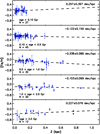 |
Fig. 15. Vertical metallicity gradients in different age bins. Symbols are the same as in Fig. 13. |
| In the text | |
|
Fig. 16. Age-metallicity relation of OCs. In our sample, the slope for OCs with age < 6 Gyr is −0.022 ± 0.008 dex Gyr−1. Three outliers are shown as triangles, and are excluded from the linear fitting procedure. |
| In the text | |
Current usage metrics show cumulative count of Article Views (full-text article views including HTML views, PDF and ePub downloads, according to the available data) and Abstracts Views on Vision4Press platform.
Data correspond to usage on the plateform after 2015. The current usage metrics is available 48-96 hours after online publication and is updated daily on week days.
Initial download of the metrics may take a while.