| Issue |
A&A
Volume 640, August 2020
|
|
|---|---|---|
| Article Number | A39 | |
| Number of page(s) | 23 | |
| Section | Extragalactic astronomy | |
| DOI | https://doi.org/10.1051/0004-6361/201936218 | |
| Published online | 07 August 2020 | |
Estimating black hole masses: Accretion disk fitting versus reverberation mapping and single epoch
1
SISSA, Via Bonomea 265, 34136 Trieste, Italy
e-mail: This email address is being protected from spambots. You need JavaScript enabled to view it.
2
INAF – Osservatorio Astronomico di Trieste, Via Tiepolo 11, 34131 Trieste, Italy
3
INAF – Osservatorio Astronomico di Brera, Via E. Bianchi 46, 23807 Merate, Italy
4
INFN – Sezione di Trieste, Via Valerio 2, 34127 Trieste, Italy
5
Dipartimento di Fisica “G. Occhialini”, Università di Milano – Bicocca, Piazza della Scienza 3, 20126 Milano, Italy
Received:
1
July
2019
Accepted:
25
May
2020
Abstract
We selected a sample of 28 Type 1 active galactic nuclei for which a black hole mass has been inferred using the reverberation mapping technique and single epoch scaling relations. All 28 sources show clear evidence of the “Big Blue Bump” in the optical-UV band whose emission is produced by an accretion disk (AD) around a supermassive black hole. We fitted the spectrum of these sources with the relativistic thin AD model KERRBB in order to infer the black hole masses and compared them with those from Reverberation mapping and Single epoch methods, discussing the possible uncertainties linked to such a model by quantifying their weight on our results. We find that for the majority of the sources, KERRBB is a good description of the AD emission for a wide wavelength range. The overall uncertainty on the black hole mass estimated through the disk fitting procedure is ∼0.45 dex (which includes the uncertainty on fitting parameters such as e.g., spin and viewing angle), comparable to the systematic uncertainty of reverberation mapping and single epoch methods; however, such an uncertainty can be ≲0.3 dex if one of the parameters of the fit is well constrained. Although all of the estimates are affected by large uncertainties, the masses inferred using the three methods are compatible if the dimensionless scale factor f (linked to the unknown kinematics and geometry of the Broad Line Region) is assumed to be larger than one. For the majority of the sources, the comparison between the results coming from the three methods favors small spin values. To check the goodness of the KERRBB results, we compared them with those inferred with other models, such as AGNSED, a model that also accounts for the emission originating from an X-ray corona: using two sources with a good data coverage in the X band, we find that the masses estimated with the two models differ at most by a factor of ∼0.2 dex.
Key words: galaxies: active / quasars: general / black hole physics / accretion / accretion disks
© ESO 2020
1. Introduction
Supermassive black holes (SMBHs) are located at the center of massive galaxies and determining their mass and spin is crucial for understanding their physical nature, the link with the host galaxy and their possible evolution in time.
Different methods have been used to estimate the mass of black holes (BHs) in active galactic nuclei (AGNs): reverberation mapping (RM, e.g., Blandford & McKee 1982; Peterson 1993; Netzer & Peterson 1997; Wandel et al. 1999; Kaspi et al. 2000; Peterson et al. 2004; Bentz et al. 2009; Fausnaugh et al. 2017; Bentz & Manne-Nicholas 2018; Shen et al. 2019; 2D velocity-delay maps, Grier et al. 2013), single epoch (SE) virial mass (e.g., Vestergaard 2002; McLure & Jarvis 2002; McLure & Dunlop 2004; Greene & Ho 2005; Vestergaard & Peterson 2006; Onken & Kollmeier 2008; Wang et al. 2009; Vestergaard & Osmer 2009; Greene et al. 2010; Shen et al. 2011; Shen & Liu 2012; Trakhtenbrot & Netzer 2012), AD fitting (e.g., Malkan 1983; Sun & Malkan 1989; Wandel & Petrosian 1988; Laor 1990; Rokaki et al. 1992; Tripp et al. 1994; Ghisellini et al. 2010; Calderone et al. 2013; Campitiello et al. 2018, 2019, hereafter C18 and C19, respectively), microlensing in gravitationally lensed quasars (QSOs, e.g., Irwin et al. 1989; Lewis et al. 1998; Richards et al. 2004; Dai et al. 2010; Mosquera & Kochanek 2011; Sluse et al. 2011; Guerras et al. 2013), polarization in broad emission lines (e.g., Savić et al. 2018), dynamical BH mass (e.g., Davies et al. 2006; Onken et al. 2007; Hicks & Malkan 2008), and the recent method based on the redshift of Fe III lines in QSOs (Mediavilla et al. 2018, 2019).
Each of them carries some uncertainties linked to the features of the system, to the parameters of the model involved for the estimates (e.g., Laor 1990; McLure & Jarvis 2002; Vestergaard & Peterson 2006; Marconi et al. 2008; Peterson 2010; Calderone et al. 2013) and clearly to the quality of data. Therefore, in order to assess the robustness of the mass estimate, it is necessary to compare the results of the different methods and possibly to calibrate the model-scaling parameters. However, this is not trivial because different approaches are based on different observables and are thus not applicable to all sources.
The aim of this work is indeed to compare the results of the AD fitting method with those of RM in order to test the reliability of AD models as an alternative approach to evaluating SMBH masses in AGNs. We chose to compare our AD fitting results with those from RM because this latter is the most accurate technique based on direct measurements related to the Broad Line Region (BLR). As a supplementary test, we also include the SE results although the method is calibrated on RM measurements.
The interpretation of the so-called “Big Blue Bump” component in the rest frame 1000–5000 Å as a “standard” AD emission has been questioned on various grounds (e.g., Koratkar & Blaes 1999; Netzer 2015). One of the debated issues, particularly relevant for this work, is related to the presence of a soft X-ray excess component observed in many objects. Some authors have developed models to account for this excess in a self-consistent way (e.g., relativistically blurred photoionized disc reflection model, Ross & Fabian 2005; Crummy et al. 2006; comptonization by an X-ray corona, e.g., Done et al. 2012; Kubota & Done 2018 – hereafter KD 18 – and references therein). Although the origin of the soft X-ray excess is not well established (e.g., Caballero-Garcia et al. 2019), in this paper we also discuss the possible effect of a warm corona above the disk that could modify the observed disk emission and therefore the determination of the BH mass.
Despite numerous criticisms, the AD fitting procedure has been widely used in the literature and shows a general agreement with the Spectral Energy Distribution (SED) and in some cases with SE BH mass estimates (e.g., Davis & Laor 2011; Laor & Davis 2011; Calderone et al. 2013; Castignani et al. 2013; Capellupo et al. 2015, 2016; Mejia-Restrepo et al. 2016; KD 18; Marculewicz & Nikolajuk 2020).
Although the aforementioned soft X-ray excess issue is still under debate, for a correct description of the AD emission, the more compelling and appropriate models are KERRBB (Li et al. 2005) and AGNSED (KD 18)1: the former describes a geometrically thin AD including all relativistic effects (e.g., frame dragging, returning radiation, light bending, gravitational redshift); the latter also takes into account the presence of an X-ray corona above the disk (even though relativistic effects such as the ones implemented in KERRBB are not fully included), thus requiring X-ray data to constrain the model parameters2. In this framework, given the large uncertainties on the physical and geometrical properties of the X-ray corona (see Sect. 5.4 and Appendix C.3 for a discussion about AGNSED) and the importance of relativistic effects, we adopted KERRBB to estimate the SMBH masses using the analytical expressions found by C18. We then considered the uncertainties of the model by comparing BH masses inferred with KERRBB with those from AGNSED for two sources with good data coverage in the X band. Significant uncertainties on the results also arise from observational issues such as absorption by dust. These possible uncertainties are discussed below along with their weight on our estimates.
The thin-disk approximation breaks down for Eddington ratios ≳0.3 (e.g., Laor & Netzer 1989) and for this reason AD models in the so-called “slim” and “thick” regimes should be considered. One of these is the relativistic model SLIMBH (Abramowicz et al. 1988; Sadowski 2009; Sadowski et al. 2009, 2011): as shown by C19, for a given set of data, the difference in the BH masses derived from KERRBB and SLIMBH is less than a factor of ∼1.2 (see the discussion in Appendix C); therefore, for the purpose of this work, we use KERRBB as a good enough approximation of the AD emission.
As already mentioned, we intend to compare the BH masses estimated from the AD fitting with those from the RM technique. This choice is due to two factors: RM is rather direct in the sense that it is not based on calibrated statistical relations but on individual measurements; and there is a significant (and still growing) number of sources with RM BH mass estimates. We selected our sample from the AGN Black Hole Mass Database (Bentz & Katz 2015)3, a compilation of published spectroscopic RM studies of AGNs, choosing sources with clear evidence of the Big Blue Bump.
The paper is structured as follows: in Sects. 2 and 3, the AGN sample and the AD fitting procedure are described in detail. Section 4 illustrates possible issues related to absorption and to uncertainties of the model. The BH masses estimated through the AD fitting are reported and compared with those from RM and SE in Sect. 5; we also discuss the possibility of estimating the BH spin and the comparison of our results with the ones inferred using AGNSED. In Sect. 6 we discuss the results and present our conclusions. In Appendices A–C, we present the basic equations used for the fits with KERRBB (Appendix A), the comparison between KERRBB and other AD models (Appendix B), the list of the sources and their fits, inferred masses and Eddington ratios (Appendix C).
In this work, we adopt a flat ΛCDM cosmology with H0 = 67.4 km s−1 Mpc−1 and ΩM = 0.315 (Planck 2018 Results).
2. Sample and data selection
Here we define the AGN sample and describe the AD fitting procedure, illustrating the possible issues related to this approach.
For all the sources of the AGN Black Hole Mass Database, we searched for the available and the most recent spectroscopic data from the near-infrared (NIR) to the far-ultraviolet (FUV) band from the public archives and literature (see Table A.1 and Appendix A)4. Among all sources, we then selected 28 (z < 0.3) with (i) a clear UV bump determined as a power-law continuum Fλ ∝ λα with a negative slope in the rest-frame wavelength range 3000–5000 Å5, (ii) wide spectroscopic coverage especially around the spectral peak, and (iii) limited variability for non-simultaneous spectra (see below). For some sources, the NIR-optical SED shows contamination by the host galaxy whose emission was taken into account in the SED modeling (see following section). For each source, spectroscopic data were corrected for Galactic extinction using the Cardelli et al. (1989) reddening law and E[B − V] from the map of Schlegel et al. (1998) with RV = 3.1.
A serious issue concerns non-simultaneous spectroscopic data that could affect the normalization of different spectra. When data did not show the same normalization, we calibrated the different data sets by adopting the following procedure: first, we considered spectroscopic data in the UV wavelength range where the peak of the AD emission should be located; then we calibrated the available FUV and optical data by matching the flux in the common wavelength range assuming that the spectral shape does not change with flux variation (see also Shang et al. 2005). The same calibration was performed on IR data (when present). In any case, the maximum mismatch amounts to ∼0.1 dex in flux (leading to an uncertainty on the derived BH mass at most by a factor of ∼0.05 dex).
Finally, spectroscopic data (especially FUSE and HUT data) were smoothed by averaging the flux in fixed wavelength bins in order to have a clearer representation of the overall emission. This latter process could have an effect on the fitting procedure and on the inferred model parameters (see following section).
3. Fitting procedure
We adopted the relativistic thin AD model KERRBB for the fitting procedure. We used GNUPLOT (non-linear least-squares Marquardt–Levenberg algorithm) to fit the rest-frame spectrum (λ − Fλ, Fig. 1) with the KERRBB model to describe the AGN continuum, adding the iron complex (e.g., Vestergaard & Wilkes 2001), some prominent emission lines (MgII, CIII, CIV, SIV and Lyα) modeled with a simple Gaussian profile, a Balmer continuum (e.g., De Rosa et al. 2014) and the template for the host-galaxy emission (Manucci et al. 2001) which can contaminate the nuclear spectrum in the NIR-optical bands.
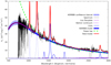 |
Fig. 1. Example of a fit of the composite FUSE – HST – KPNO spectrum of the source PG 0953+414 (from Shang et al. 2005). The modeling performed with KERRBB (thick blue line) describes the AGN continuum, the iron complex (purple line), the Balmer continuum (purple dashed line), and some prominent emission lines (MgII, CIII, CIV, SiIV, Lyα) described by a simple Gaussian profile (blue lines). The red line represents the sum of all these components. The green dashed line is a standard power-law continuum (slope α = −1.77): for λ > 1300 Å, the KERRBB model overlaps the power-law rather well within the average confidence interval (∼0.05 dex, blue shaded area) and is not affected significantly by the presence of lines or other spectral features. Abundant interstellar absorption lines at λ < 1000 Å have a negligible effect on the determination of the spectral peak emission (see Sect. 4). |
As a comparison, we also performed a standard fit using a power-law to describe the AGN continuum: in Fig. 1 we show, as an example, the results of both fits. It is clear that the two continua overlap well for λ > 1300 Åwhile the AD model turns over around the spectral peak. Even if this latter is not covered by data, it can be constrained using the curvature of the spectrum at smaller frequencies. Spectral features, such as strong emission or absorption lines, have no drastic effects on the overall KERRBB fit, even at short wavelengths where the spectrum peak is located (see following section)6.
Each fit constrains the spectrum peak position which is essential to infer the BH mass (see Appendix B): in the ν − νLν representation, both the peak frequency νp and luminosity νpLνp have a mean uncertainty of ∼0.05 dex (represented with a blue shaded area in Fig. 1 and in all the Figures reporting the spectral fits, Figs. A.1–A.28). This confidence interval translates to an average uncertainty of ∼0.1 dex on the BH mass (for a fixed BH spin and viewing angle – see Sect. 5.1).
4. Caveats: data uncertainties
In this section we discuss the possible effects of absorption by gas or dust on the overall AD spectrum shape.
First, for some ground-based telescopes, the available spectrum can be subjected to absorption due to sky regions with low transparency. Even if these regions are subtracted, our best fit does not change significantly and remains inside the average confidence interval (∼0.05 dex).
Spectra show some absorption features caused by the interstellar medium, especially at frequencies Log ν/Hz ≳ 15.4: if these blended lines are smoothed or not subtracted from the spectrum appropriately, the AGN continuum can be underestimated, leading to an incorrect evaluation of the spectral peak position (i.e., shifting νp to smaller values and leading to an overestimation of the BH mass). In order to understand if these spectral features have a relevant effect on our results, we performed the same fitting procedure described in the previous section, choosing only the frequency range Log ν/Hz ≲ 15.4; even if the spectral range is reduced, the curvature of the spectrum at smaller frequencies can still be used to constrain the peak position. We find that the new peak frequencies are on average larger than the previous ones (inferred considering the whole available spectral range) but consistent with them within a range of ∼0.05 dex, while the luminosities are similar. The inferred new BH masses are inside the average confidence interval of ∼0.1 dex (defined by the spectrum peak uncertainty).
The intergalactic medium (IGM) could also modify the spectrum shape (especially for high-redshift sources) at frequencies Log ν/Hz ≳ 15.4. For the redshift range spanned by our sample the correction from IGM absorption is negligible (see Madau 1995; Haardt & Madau 2012; Castignani et al. 2013) except for the two high-redshift sources, PG 1247+267 and S5 0836+71. For these latter, we performed this correction and showed the results in Figs. A.23–A.28, respectively.
An important effect that could modify the spectral UV shape concerns dust absorption: if present, this could lead to an incorrect BH mass estimate. The absorption could be caused by the dusty torus surrounding the AD, or dust in the host galaxy interstellar medium (ISM)7. Given that our sample is composed of Type 1 QSOs (FWHM > 1000 km s−1 for the most prominent lines; e.g., Antonucci 1993) we do not expect any (strong) absorption from the dusty torus, which is assumed to have an average opening angle of ∼45°. For this reason, in order to infer the BH mass, we assumed that each source was observed with a viewing angle θv ≤ 45° (see Appendix for results).
However, we checked the goodness of our fit by considering the possible intrinsic reddening by the host galaxy ISM. To do so, we followed the work by Baron et al. (2016), who found an analytical expression to infer the amount of absorption (in terms of E[B − V]) as a function of the rest frame spectrum slope αν in the wavelength range 3000–5100 Å. We find that for the majority of the sample, the correction is small (E[B − V]< 0.05 mag) and could lead to a decrease of the BH mass by a factor ≲0.1 dex. The extinction found is consistent with what is thought to be the average value for AGN (E[B − V] ∼ 0.05 − 0.1 mag; e.g., Koratkar & Blaes 1999).
For a more complete analysis of the possible UV dust absorption, for each source we used the extinction law of Czerny et al. (2004) and assumed that the slope of the corrected, de-reddened spectrum at wavelength < 2000 Åhad to be softer than the theoretical value Fν ∝ ν1/3. In this way, we find an upper limit for the correction (on average E[B − V] ∼ 0.20 mag) that leads to a decrease of the BH mass obtained through the SED fitting procedure at most by a factor of ∼0.3 dex (since the spectrum peak position changes due to the correction).
As explained above, we do not expect such a strong UV absorption because we are dealing with Type 1 QSOs. Moreover, for what concerns the correction found by Baron et al. (2016) regarding ISM dust absorption, possible deviations from the average continuum slope could be caused by other factors connected to the BH physics, such as the BH mass, the accretion rate, the spin, and the system orientation (e.g., Hubeny et al. 2000; Davis & Laor 2011). Therefore, we did not consider any correction from dust absorption, and are confident that our results are inside the estimated BH mass confidence interval (even if the intrinsic extinction is taken into account).
5. Results
In this section, we show the results coming from the SED fitting procedure. We used the analytical expressions found by C18 in order to infer the BH mass and the Eddington ratio (reported in Table A.2) using KERRBB, in the spin range 0 ≤ a ≤ 0.998 and for a viewing angle θv ≤ 45°. As shown by the authors, the space of KERRBB solutions is degenerate and by using different parameters (M, a and accretion rate) appropriately, it is possible to describe the same set of data.
We compare KERRBB BH masses MBH, Fit to the ones obtained through RM and from SE equations: we fit the relation between our estimates linearly, that is, the virial product (VP; computed with RM results) and SE estimates (i.e., Log MBH, Fit = Log M[VP or SE]+Log f). The VP is the base of all virial-based mass measurements:
 (1)
(1)
where τLT is the light-travel time (i.e., the time related to the emission-line response delayed with respect to changes in the continuum) and σline is the line velocity dispersion (or the line FWHM; e.g., Ho 1999; Wandel et al. 1999). The factor f corresponds to the geometrical factor fBLR when the comparison is performed with the VP, while it is merely a multiplicative factor in the case of SE measurements, for which fBLR has already be chosen in literature as an average value (∼1, Vestergaard & Peterson 2006). Many authors have calibrated the geometrical factor by comparing BH masses obtained with different approaches (see Bentz & Katz 2015, and references therein)8. Some authors use fBLR = 3 (3/4), if the VP is computed using σline (FWHM), considering a spherical distribution of BLR clouds in randomly orientated orbits (Netzer 1990; Wandel et al. 1999; Kaspi et al. 2000)9. The RM technique estimates have a systematic uncertainty of ∼0.5 dex (as the SE one, Vestergaard & Osmer 2009).
5.1. Black hole mass uncertainty
The total uncertainty on the KERRBB BH mass inferred from the SED fitting procedure is ∼0.45 dex (comparable to the systematic uncertainties on the RM and SE estimates: ∼0.5 dex). This uncertainty has to be considered as a confidence interval in which the BH mass inferred with KERRBB lies and is connected to different quantities involved in the fitting procedure, namely the BH Spin, in the range 0 ≤ a ≤ 0.998; the viewing angle of the system, in the range 0° ≤ θv ≤ 45°; and the uncertainty on the spectral peak frequency and luminosity.
Assuming that there is no dust absorption, the BH mass changes by ∼0.5 dex going from a = 0 to a = 0.998 (for a fixed viewing angle), and by ∼0.2 dex going from θv = 0° to θv = 45° (for a fixed spin). Taking as a reference value the arithmetic mean of the BH mass in both the spin and θv ranges, the overall uncertainty is ∼0.35 dex. Moreover, the confidence interval on the spectral peak position (∼0.05 dex) leads to an additional uncertainty of ∼0.1 dex on the BH mass estimate. However, if the spectral peak is well constrained (and/or the viewing angle is known), the mean uncertainty on the AD BH mass estimates can be ≲0.3 dex.
5.2. Black hole mass comparison
Figure 2 shows the comparison between our BH mass estimates inferred from the SED fitting procedure with KERRBB and the VPs computed using the Hβ velocity dispersion σline (left panel) and the FWHM (right panel; as we used the CIV line to compute the VPs, we excluded PG 1247+267 and S5 0836+71 from the fit for consistency). The comparison between the VP computed using the velocity dispersion and the FWHM is shown because several authors claimed that the ratio FWHM/σline is not necessarily a constant (e.g., Collin et al. 2006, Peterson 2011): for our sample, we find FWHM/σlines ∼ 2 with a large dispersion (∼0.5 dex). Instead, Fig. 3 shows the comparison between our results and the BH masses computed using the SE relations of Vestergaard & Peterson (2006).
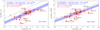 |
Fig. 2. Comparison between KERRBB BH mass estimates MBH, fit (inferred from the SED fitting procedure; each dot corresponds to the mean value computed using the extreme estimates given by the uncertainties) and the VPs calculated using the Hβ velocity dispersion σline (left panel) and the FWHM (right panel). We averaged all the VPs computed using data from different authors (see Table A.2; PG 1247+267 and S5 0836+71 are marked with green dots). The blue shaded area corresponds to the set of best fits between MBH, Fit and VP after considering all possible spin values between 0 and 0.998 (equations in blue on the plot are the two extreme cases; the uncertainty on the slope is ∼20%). Assuming that Log MBH, fit = LogVP + Log f, we found the scale factor f, labeled on the plot in red for the two extreme spin values. Uncertainty bars in both plots are ∼0.45 dex and ∼0.5 dex for MBH, fit and VPs respectively, and the black dashed line is the 1:1 line. |
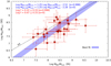 |
Fig. 3. Comparison between the KERRBB BH mass estimates MBH, fit (inferred from the SED fitting procedure) and the SE BH masses MBH, SE computed using the equation of Vestergaard & Peterson (2006) and the Hβ line (we excluded the two high-redshift sources, PG 1247+267 and S5 0836+71, for which we only have information on the CIV line; see Table A.2). The blue shaded area, the dashed black line, the reported labels, and the uncertainty bars are the same as in Fig. 2. |
From the analysis of those results, we find that both the VPs and the SE estimates are systematically smaller than the KERRBB estimates by a factor f depending on the BH spin. For VP(σline) and VP(FWHM), assuming a BH spin a = 0 (0.998), we find Log f = 0.81 (1.17)±0.15 and Log f = 0.27 (0.63)±0.15, respectively. As in this case f is identified as the geometrical factor fBLR (beginning of Sect. 5), the range we find by using VP(σline) is consistent for example with fBLR = 5.5 ± 1.8 (Onken et al. 2004; see also Li et al. 2018 for other reference values). In both cases, the compatibility is more compelling if, on average, BH spins are assumed to be small. For SE estimates, we find Log f = 0.07 (0.43)±0.15, assuming a BH spin a = 0 (0.998), partially consistent with the recent work by Marculewicz & Nikolajuk (2020). This result is similar to the one found for VP(FWHM): this is due to the use of a geometrical factor fBLR ∼ 1 and FWHM measurements inside virial equations of Vestergaard & Peterson (2006). Therefore SE and VP(FWHM) are almost the same (within uncertainties).
From Fig. 2 (left panel), it is clear that KERRBB mass estimates are systematically larger than the corresponding VPs: from the fit, a better compatibility is reached if a scale factor of the order of ∼10 is assumed, in agreement with the recent paper by Pozo Nuñez et al. (2019). Nonetheless, our results are still compatible with those estimated using RM if, for these latter, a geometrical factor of less than ten is considered. Figure 4 shows our KERRBB BH estimates compared with the ones from SE and RM (computed using the velocity dispersion σline and different geometrical factors fBLR = 2.8 − 5.5, from Graham et al. 2011 and Onken et al. 2004, respectively): about 70% of the sources show a good compatibility between the three results within uncertainties (∼0.5 dex, on average) favoring smaller KERRBB masses and therefore low spin values. See Sect. 5.4 and Appendix C for a comparison between KERRBB results and those inferred with other models..
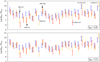 |
Fig. 4. Comparison between the BH masses computed from the SED fitting procedure with KERRBB (blue) and the SE (orange) and RM estimates (red, inferred with σline and a geometrical factor fBLR = 2.8 − 5.5, Graham et al. 2011top panel and Onken et al. 2004bottom panel). The average uncertainty for all the measurements is ∼0.5 dex (the results related to each source are plotted in the same order as listed in the Tables of Appendix A). |
5.3. Spin estimate
Given the large uncertainties involved in each method to infer the BH mass, an estimate of the BH spin is still a hard task. In principle, the comparison of two or more independent BH masses with relativistic AD model results could be an alternative way to constrain the BH spin (e.g., see C19).
For the majority of the sources, the comparison showed that small spin values are favored. Instead, for a couple of sources (MRK 1383, S5 0836+71), the comparison between RM, SE, and KERRBB results (within uncertainties) led to the conclusion that the BH spin must be high (we found a lower limit a > 0.6). However, as mentioned above, because uncertainties on the fitting procedure, on the parameters of the AD, and on the RM measurements (as well as other methods) are still large, we suggest caution be taken when considering a BH spin estimate based on the comparison of different BH masses.
5.4. X-ray corona above the disk: modifications in the BH mass estimates
Estimations of the BH mass using the SED fitting procedure could be affected by the presence of a hot Corona above the disk: this structure is thought to be compact (e.g., Miniutti & Fabian 2004; Done et al. 2012; Reis & Miller 2013; Sazonov et al. 2012; Lusso & Risaliti 2017) and responsible for the emission in the X band and for the soft X-ray excess observed in many AGNs (e.g., Koratkar & Blaes 1999). In principle, if this structure scatters a fraction of the disk radiation, the observed disk luminosity could be dimmer than the intrinsic one, leading to an incorrect mass estimate (i.e., the spectrum peak position could be different from the intrinsic one).
In order to check this possibility, we compared our results with those of the relativistic model AGNSED (KD 18), which also takes into account also the presence of an X-ray corona above the disk in a self-consistent way. It is important to note that, contrary to KERRBB, AGNSED does not include relativistic effects, such as light bending and gravitational redshift, which may have a significant effect on both the AD and the corona emissions; however, for small values of the BH spin and θv, those effects should have a minor weight on the results.
For the fitting procedure, we used the sources NGC 5548 and MRK 509 (see Appendix C for details) also studied by KD 18. We found that, as for KERRBB, the modeling with AGNSED of the optical-UV-X SED is degenerate: by changing the model parameters (i.e., BH mass, spin, Eddington ratio, corona size) appropriately, it is possible to reproduce the same set of data (for some reference values, see Fig. C.1).
For NGC 5548, results from both models are compatible while for MRK 509, KERRBB BH masses are larger than the AGNSED ones by a factor ≲0.2 dex (Fig. C.2, right panel). We argue that for NGC 5548, the absence of relativistic effects in AGNSED is balanced out by modeling a large corona above the disk, leading to the same BH mass. Instead, for MRK 509, the smaller X-ray corona leads to different results because it does not compensate the differences between the two models.
In general, KERRBB observed disk luminosity is dimmer than the intrinsic one because of a compact corona located in the inner region of the disk, the presence of which modifies the AD emission and leads to an overestimated BH mass. By correcting the KERRBB disk lumminosity by a factor ≲0.2 dex, results from the two models related to MRK 509 show better compatibility (see Appendix C for more details about this correction).
The partial compatibility between KERRBB and AGNSED shows that BH masses estimated though the SED fitting procedure clearly depend on the adopted model and their physical background. Despite these findings, KERRBB results for both sources are still compatible with SE and RM ones within uncertainties (Fig. 4). Moreover, results presented by KD 18 are compatible with ours for what concerns the BH spin: taking their finding for the BH masses as reference values, both their results and ours favor low values of a.
6. Discussion and conclusions
We used the relativistic thin AD model KERRBB (Li et al. 2005) to infer the BH masses of 28 sources from the AGN Black Hole Mass Database (Bentz & Katz 2015). These sources have a BH mass estimate from the RM studies and show clear evidence in the UV band of the so-called Big Blue Bump produced by the radiation coming from an AD around a SMBH. Since we did not have information about the viewing angle for the majority of them, we assumed that the Type 1 QSOs were observed with θv ≤ 45° in order to avoid the absorption from the dusty torus (assumed to have an average opening angle of ∼45°). Our results can be summarized as follows:
-
The majority of the sources of our sample show a good match between data and the modeling with KERRBB. The modeling led to a relatively good estimate of the spectrum peak position (i.e., peak frequency and luminosity; see Appendix B) with a small uncertainty (∼0.05 dex on average).
-
The total uncertainty related to the AD BH mass estimates is ∼0.45 dex, which is connected to the unknown BH spin (in the range 0 ≤ a ≤ 0.998), the viewing angle (θv ≤ 45°), and the uncertainty on the peak position from the fitting procedure. If the quality of the data is high and either the spectral peak or the viewing angle of the system are well constrained (with an uncertainty of less then ∼10%), the mean uncertainty is reduced to ≲0.3 dex, which is smaller than the systematic uncertainties on both the RM and SE estimates (∼0.5 dex, e.g., Vestergaard & Osmer 2009);
-
Our BH mass estimates with KERRBB are systematically larger than the corresponding VPs (computed using both the velocity dispersion σline and the FWHM). We computed the difference through a scale factor f and found Log f ≲ 1.2 (depending on the BH spin – Fig. 2), which is also in agreement with the recent paper by Pozo Nuñez et al. (2019). A similar result is found from the comparison between our results and BH masses inferred with SE equations (Log f ≲ 0.5, Fig. 3).
-
Despite these findings, assuming a geometrical factor in the range fBLR = 2.8 − 5.5 (from Graham et al. 2011 and Onken et al. 2004, respectively), we find a compatibility between RM, SE, and KERRBB results for ∼70% (Fig. 4).
-
In principle, a comparison between independent BH mass estimates (e.g., RM, SE) and the ones coming from the SED fitting procedure with a relativistic AD model could lead to an estimate of BH spin (e.g., C19): for a couple of sources we find a lower limit (a > 0.6) but, for the majority of the sample, low spin values are favored. These results must be considered with caution because the uncertainties on the different parameters involved in the fitting procedure and RM (or SE) measurements are still large.
-
Assuming that the BH masses estimated through the AD fitting procedure are correct, the geometrical factor must be large (Fig. 2) in order to compensate for the difference with the corresponding VPs. Assuming a disk-like BLR (e.g., Collin et al. 2006; Decarli et al. 2008), the geometrical factor related to the VP (computed using the FWHM) is:
![Mathematical equation: $$ \begin{aligned} f_{\rm BLR} = \frac{1}{4\ \Bigl [ (\sin \theta _{\rm v})^2 + (H/r)^2 \Bigl ]} \end{aligned} $$](/articles/aa/full_html/2020/08/aa36218-19/aa36218-19-eq2.gif) (2)
(2)where H/r is the height-to-radius ratio (i.e., thickness) of the BLR. The range of scale factors found in this work is consistent with a BLR seen with a viewing angle < 30° (consistent with Type 1 QSOs) and a thickness H/r < 0.5 (consistent with the results of Mejia-Restrepo et al. 2016; see Fig. 5).
-
Black hole mass measurements through the SED fitting procedure could be affected by the presence of a hot X-ray corona above the AD. We checked this possibility by comparing our KERRBB results with those from the relativistic model AGNSED (KD 18) that accounts also for the X-ray emission in a self-consistent way. We used two sources, NGC 5548 and MRK 509, and find that for NGC 5548, results from both models are compatible while for MRK 509, KERRBB BH masses are larger by a factor ≲0.2 dex with respect to those inferred with AGNSED. We argue that the possible presence of an X-ray corona above the disk modifies the emission of this latter leading to an overestimated BH mass; we corrected the emission following the simple prescription described in Appendix C and reaching a relatively good compatibility between the two results. However, despite this correction, if uncertainties on RM and SED fitting estimates are taken into account, both our results and those of KD 18 favor small BH spin values.
-
The comparison between all those results suggests that the systematic discrepancy between KERRBB and RM (or SE) masses (i.e., the large value of the factor f – see Fig. 2) could possibly be related to the choice of the AD model adopted in the SED fitting procedure. However, the partial compatibility between KERRBB and AGNSED leads to the conclusion that results are strictly connected to the geometry of the X-ray corona and to the relativistic AD radiation pattern, which are not both included in the models used here. Furthermore, a comparison between different models is necessary in order to understand their differences and to improve them.
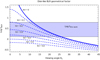 |
Fig. 5. Geometrical factor fBLR computed using Eq. (2) (e.g., Collin et al. 2006; Decarli et al. 2008) as a function of the viewing angle for different BLR thickness H/r. The blue shaded area is the scale factor range found in this work (related to VPs computed using the FWHM; see Fig. 2, right panel). The comparison leads to a range of θv and H/r consistent with the work of Mejia-Restrepo et al. (2016). |
Despite the large uncertainties involved in the fitting procedure and RM (or SE) measurements, KERRBB showed a good agreement with data, strengthening the choice of AD models as an alternative method both to described the observed SEDs and to infer the mass of SMBHs. For what concerns these latter arguments, the choice of the AD model is crucial even though we found similar results using different models. Nonetheless, although few attempts are discussed in this work, the uncertainties involved in these kinds of measurements are still too large to have precise information on the BH accretion and spin from the comparison between different methods. A larger sample of sources with RM measurements and a clear prominent AD emission are necessary to strengthen these findings, to improve AD models for what concerns the modeling of the observed SEDs, and possibly to obtain more information on the BH accretion and rotation.
Both models are implemented in XSPEC (Arnaud 1996).
Relativistic effects due to large spin values modify the AD emission shape with respect to the “standard” one (e.g., Shakura & Sunyaev 1973; Novikov & Thorne 1973): AGNSED does not include all such effects possibly affecting the predicted disk and corona emissions.
See also http://www.astro.gsu.edu/AGNmass/
We also collected some photometric data (GALEX, Vizier, NED), not taken into account in the fitting procedure because (i) they might be contaminated by emission lines or by some kind of absorption and (ii) their statistical weight in the fit is negligible.
Only two sources (PG 1247+267, S5 0836+71) are at z ∼ 2. For them, spectroscopic data cover only the spectrum peak position.
As an additional test, we used two Gaussians to fit the broad base of the most prominent lines: we still have no drastic effects on the AGN continuum which remains inside the confidence interval of ∼0.05 dex.
Recent works (e.g., Leftley et al. 2018) show that ∼50 − 80% of the MIR emission originates primarily from polar regions instead of from an equatorial dust distribution. This can have an effect on the observed disk luminosity which would be dimmer with respect the intrinsic one since part of its radiation is intercepted by the polar dust.
See Li et al. (2018) for a list of fBLR values found in literature.
The line velocity dispersion is often identified either as the line FWHM or as the σ of the Gaussian profile used to fit the emission line.
The total disk luminosity Ld = ηṀc2 differs from the observed disk luminosity (i.e., the frequency integrated AD luminosity,  ) because of relativistic effect described by ℱ (for details see C18).
Following the work of Davis & Laor (2011), from their Eq. (5), we have νLν,opt ∝ (ṀM)2/3, where νLν,opt is the luminosity at Log ν/Hz ∼ 14.8. By using Eqs. (B.1)–(B.3), it is possible to write  : this luminosity must be constant before and after the correction with the factor α therefore we can write
  . From this latter, knowing that νp, αLν, α = νpLνp/α, we finally have νp, α ∼ νpα−3/4.
Acknowledgments
We thank the anonymous referee for her/his constructive comments and suggestions, useful to improve the manuscript.
References
- Abramowicz, M., Czerny, B., Lasota, J. P., & Szuszkiewicz, E. 1988, ApJ, 332, 646 [NASA ADS] [CrossRef] [Google Scholar]
- Antonucci, R. 1993, ARA&A, 31, 473 [Google Scholar]
- Arnaud, K. A. 1996, in Astronomical Data Analysis Software and Systems V, eds. G. H. Jacoby, & J. Barnes, ASP Conf. Ser., 101, 17 [Google Scholar]
- Asmus, D., Hönig, S. F., & Gandhi, P. 2016, ApJ, 822, 109 [NASA ADS] [CrossRef] [Google Scholar]
- Baron, D., Stern, J., Poznanski, D., & Netzer, H. 2016, ApJ, 832, 8 [CrossRef] [Google Scholar]
- Bechtold, J. A., Dobrzycki, B., Wilden, B., et al. 2002, ApJS, 140, 143 [NASA ADS] [CrossRef] [Google Scholar]
- Bentz, M. C., & Katz, S. 2015, PASP, 127, 67 [NASA ADS] [CrossRef] [Google Scholar]
- Bentz, M. C., & Manne-Nicholas, E. 2018, ApJ, 864, 146 [NASA ADS] [CrossRef] [EDP Sciences] [Google Scholar]
- Bentz, M. C., Walsh, J. L., Barth, A. J., et al. 2009, ApJ, 705, 199 [NASA ADS] [CrossRef] [Google Scholar]
- Bentz, M. C., Horenstein, D., Bazhaw, C., et al. 2014, ApJ, 796, 8 [NASA ADS] [CrossRef] [Google Scholar]
- Blandford, R. D., & McKee, C. F. 1982, ApJ, 255, 419 [NASA ADS] [CrossRef] [EDP Sciences] [Google Scholar]
- Boroson, T. A., & Green, R. F. 1992, ApJS, 80, 109 [NASA ADS] [CrossRef] [Google Scholar]
- Caballero-Garcia, M. D., Dovciak, M., Bursa, M., et al. 2019, ArXiv e-prints [arXiv:1901.04357] [Google Scholar]
- Calderone, G., Ghisellini, G., Colpi, M., & Dotti, M. 2013, MNRAS, 431, 210 [NASA ADS] [CrossRef] [Google Scholar]
- Campitiello, S., Ghisellini, G., Sbarrato, T., & Calderone, G. 2018, A&A, 612, A59 [NASA ADS] [CrossRef] [EDP Sciences] [Google Scholar]
- Campitiello, S., Celotti, A., Ghisellini, G., & Sbarrato, T. 2019, A&A, 625, A23 [CrossRef] [EDP Sciences] [Google Scholar]
- Capellupo, D. M., Netzer, H., Lira, P., et al. 2015, MNRAS, 446, 3427 [NASA ADS] [CrossRef] [Google Scholar]
- Capellupo, D. M., Netzer, H., Lira, P., et al. 2016, MNRAS, 460, 212 [NASA ADS] [CrossRef] [Google Scholar]
- Cardelli, J. A., Clayton, G. C., & Mathis, J. S. 1989, ApJ, 345, 245 [NASA ADS] [CrossRef] [Google Scholar]
- Castelló-Mor, N., Netzer, H., & Kaspi, S. 2016, MNRAS, 458, 1839 [NASA ADS] [CrossRef] [Google Scholar]
- Castignani, G., Haardt, F., Lapi, A., et al. 2013, A&A, 560, A28 [NASA ADS] [CrossRef] [EDP Sciences] [Google Scholar]
- Collin, S., Kawagushi, T., Peterson, B., & Vestergaard, M. 2006, A&A, 456, 75 [NASA ADS] [CrossRef] [EDP Sciences] [Google Scholar]
- Crummy, J., Fabian, A. C., Gallo, L., & Ross, R. R. 2006, MNRAS, 365, 1067 [NASA ADS] [CrossRef] [Google Scholar]
- Cunningham, C. T. 1975, ApJ, 202, 788 [NASA ADS] [CrossRef] [Google Scholar]
- Czerny, B., Li, J., Loska, Z., & Szczerba, R. 2004, MNRAS, 348, L54 [NASA ADS] [CrossRef] [Google Scholar]
- Dai, X., Kochanek, C. S., Chartas, G., et al. 2010, ApJ, 709, 278 [NASA ADS] [CrossRef] [Google Scholar]
- Davies, R. I., Thomas, J., Genzel, R., et al. 2006, ApJ, 646, 754 [NASA ADS] [CrossRef] [Google Scholar]
- Davis, S. W., & Laor, A. 2011, ApJ, 728, 98 [CrossRef] [Google Scholar]
- Decarli, R., Dotti, M., Fontana, M., & Haardt, F. 2008, MNRAS, 386, L15 [NASA ADS] [Google Scholar]
- Denney, K. D., Peterson, B. M., Pogge, R. W., et al. 2010, ApJ, 721, 715 [NASA ADS] [CrossRef] [Google Scholar]
- De Rosa, G., Venemans, B. P., Decarli, R., et al. 2014, ApJ, 790, 145 [NASA ADS] [CrossRef] [Google Scholar]
- De Rosa, G., Fausnaugh, M. M., Grier, C. J., et al. 2018, ApJ, 866, 133 [NASA ADS] [CrossRef] [Google Scholar]
- Done, C., Davis, S. W., Jin, C., Blaes, O., & Ward, M. 2012, MNRAS, 420, 1848 [NASA ADS] [CrossRef] [Google Scholar]
- Du, P., Brotherton, M. S., Wang, K., Huang, Z. P., et al. 2018, ApJ, 869, 142 [CrossRef] [Google Scholar]
- Fausnaugh, M. M., Grier, C. J., Bentz, M. C., et al. 2017, ApJ, 840, 97 [NASA ADS] [CrossRef] [Google Scholar]
- Ghisellini, G., Ceca, R. D., Volonteri, M., et al. 2010, MNRAS, 405, 387 [NASA ADS] [Google Scholar]
- Graham, A. W., Onken, C. A., Athanassoula, E., & Combes, F. 2011, MNRAS, 412, 221 [Google Scholar]
- Greene, J. E., & Ho, L. C. 2005, ApJ, 630, 122 [NASA ADS] [CrossRef] [Google Scholar]
- Greene, J. E., Peng, C. Y., Kim, M., et al. 2010, ApJ, 721, 26 [NASA ADS] [CrossRef] [Google Scholar]
- Grier, C. J., Peterson, B. M., Pogge, R. W., et al. 2012, ApJ, 755, 60 [NASA ADS] [CrossRef] [Google Scholar]
- Grier, C. J., Peterson, B. M., Horne, K., et al. 2013, ApJ, 764, 47 [NASA ADS] [CrossRef] [Google Scholar]
- Grier, C. J., Pancoast, A., Barth, A. J., et al. 2017, ApJ, 849, 146 [NASA ADS] [CrossRef] [Google Scholar]
- Guerras, E., Mediavilla, E., Jimenez-Vicente, J., et al. 2013, ApJ, 764, 160 [NASA ADS] [CrossRef] [Google Scholar]
- Haardt, F., & Madau, P. 2012, ApJ, 746, 125 [NASA ADS] [CrossRef] [Google Scholar]
- Haas, M., Chini, R., Ramolla, M., et al. 2011, A&A, 535, A73 [NASA ADS] [CrossRef] [EDP Sciences] [Google Scholar]
- Hicks, E. K. S., & Malkan, M. A. 2008, ApJS, 174, 31 [NASA ADS] [CrossRef] [Google Scholar]
- Ho, L. C. 1999, in Observational Evidence for Black Holes in the Universe, ed. S. K. Chakrabarti (Dordrecht: Kluwer), 157 [NASA ADS] [CrossRef] [Google Scholar]
- Ho, L. C., Filippenko, A. V., & Sargent, W. L. 1995, ApJS, 98, 477 [NASA ADS] [CrossRef] [Google Scholar]
- Hubeny, I., Agol, E., Blaes, O., & Krolik, J. H. 2000, ApJ, 533, 710 [NASA ADS] [CrossRef] [Google Scholar]
- Irwin, M. J., Webster, R. L., Hewett, P. C., et al. 1989, AJ, 98, 1989 [NASA ADS] [CrossRef] [Google Scholar]
- Jin, C., Ward, M., Done, C., & Gelbord, J. 2012, MNRAS, 420, 1825 [NASA ADS] [CrossRef] [Google Scholar]
- Jones, D. H., Read, M. A., Saunders, W., et al. 2009, MNRAS, 399, 683 [NASA ADS] [CrossRef] [Google Scholar]
- Kaspi, S., Smith, P. S., Netzer, H., et al. 2000, ApJ, 533, 631 [NASA ADS] [CrossRef] [Google Scholar]
- Kaspi, S., Brandt, W. N., Maoz, D., et al. 2007, ApJ, 659, 997 [NASA ADS] [CrossRef] [Google Scholar]
- Kennicutt, R. C. 1992, ApJ, 388, 310 [NASA ADS] [CrossRef] [Google Scholar]
- Kinney, A. L., Bohlin, R. C., Blades, J. C., & York, D. G. 1991, ApJS, 75, 645 [NASA ADS] [CrossRef] [Google Scholar]
- Kollatschny, W., & Zetzl, M. 2013, A&A, 558, A26 [NASA ADS] [CrossRef] [EDP Sciences] [Google Scholar]
- Koratkar, A., & Blaes, O. 1999, PASP, 111, 1 [NASA ADS] [CrossRef] [Google Scholar]
- Kubota, A., & Done, C. 2018, MNRAS, 480, 1247 [NASA ADS] [CrossRef] [Google Scholar]
- Landt, H., Elvis, M., Ward, M. J., et al. 2011, MNRAS, 414, 218 [NASA ADS] [CrossRef] [Google Scholar]
- Landt, H., Ward, M. J., Peterson, B. M., et al. 2013, MNRAS, 432, 113 [NASA ADS] [CrossRef] [Google Scholar]
- Laor, A. 1990, MNRAS, 246, 369 [NASA ADS] [Google Scholar]
- Laor, A., & Davis, S. 2011, ArXiv e-prints [arXiv:1110.0653] [Google Scholar]
- Laor, A., & Netzer, H. 1989, MNRAS, 238, 897 [NASA ADS] [CrossRef] [Google Scholar]
- Lawrence, C. R., Zucker, J. R., Readhead, A. C. S., et al. 1996, ApJS, 107, 541 [NASA ADS] [CrossRef] [Google Scholar]
- Leftley, J. H., Tristram, K. R. W., Hönig, S. F., et al. 2018, ApJ, 862, 17 [CrossRef] [Google Scholar]
- Lewis, G. F., Irwin, M. J., Hewett, P. C., & Foltz, C. B. 1998, MNRAS, 295, 573 [NASA ADS] [CrossRef] [Google Scholar]
- Li, L.-X., Zimmerman, E. R., Narayan, R., & McClintock, J. E. 2005, ApJ, 157, 335 [Google Scholar]
- Li, Y. R., Songsheng, Y. Y., Qiu, J., Hu, C., et al. 2018, ApJ, 869, 137 [CrossRef] [Google Scholar]
- López-Gonzaga, N., Burtscher, L., Tristram, K. R. W., Meisenheimer, K., & Schartmann, M. 2016, A&A, 591, A47 [NASA ADS] [CrossRef] [EDP Sciences] [Google Scholar]
- Lusso, E., & Risaliti, G. 2017, A&A, 602, A79 [NASA ADS] [CrossRef] [EDP Sciences] [Google Scholar]
- Madau, P. 1995, ApJ, 441, 18 [NASA ADS] [CrossRef] [Google Scholar]
- Mejia-Restrepo, J. E., Trakhtenbrot, B., Lira, P., et al. 2016, MNRAS, 460, 187 [NASA ADS] [CrossRef] [Google Scholar]
- Malkan, M. A. 1983, ApJ, 268, 582 [NASA ADS] [CrossRef] [Google Scholar]
- Manucci, F., Basile, F., Poggianti, B. M., et al. 2001, MNRAS, 326, 745 [NASA ADS] [CrossRef] [Google Scholar]
- Marconi, A., Axon, D. J., Maiolino, R., et al. 2008, ApJ, 678, 693 [NASA ADS] [CrossRef] [Google Scholar]
- Marculewicz, M., & Nikolajuk, M. 2020, ApJ, 897, 117 [CrossRef] [Google Scholar]
- McLure, R. J., & Dunlop, J. S. 2004, MNRAS, 352, 1390 [NASA ADS] [CrossRef] [Google Scholar]
- McLure, R. J., & Jarvis, M. J. 2002, MNRAS, 337, 109 [NASA ADS] [CrossRef] [Google Scholar]
- Mediavilla, E., Jiménez-Vicente, J., Fian, C., et al. 2018, ApJ, 862, 104 [NASA ADS] [CrossRef] [Google Scholar]
- Mediavilla, E., Jiménez-Vicente, J., Mejía-Restrepo, J., et al. 2019, ApJ, 880, 96 [CrossRef] [Google Scholar]
- Miniutti, G., & Fabian, A. C. 2004, MNRAS, 349, 1435 [NASA ADS] [CrossRef] [Google Scholar]
- Mosquera, A. M., & Kochanek, C. S. 2011, ApJ, 738, 96 [NASA ADS] [CrossRef] [Google Scholar]
- Netzer, H. 1990, in Active Galactic Nuclei, eds. T. J.-L. Courvoisier, & M. Mayor, 137 [Google Scholar]
- Netzer, H. 2015, ARA&A, 53, 365 [NASA ADS] [CrossRef] [Google Scholar]
- Netzer, H., & Peterson, B. M. 1997, Astrophys. Space Sci. Lib., 218, 85 [CrossRef] [Google Scholar]
- Novikov, I. D., & Thorne, K. S. 1973, in Black Holes, eds. C. De Witt, & B. De Witt (New York: Gordon and Breach), 343 [Google Scholar]
- Onken, C. A., & Kollmeier, J. A. 2008, ApJ, 689, L13 [NASA ADS] [CrossRef] [Google Scholar]
- Onken, C. A., Ferrarese, L., Merritt, D., et al. 2004, ApJ, 615, 645 [NASA ADS] [CrossRef] [Google Scholar]
- Onken, C. A., Valluri, M., Peterson, B. M., et al. 2007, ApJ, 670, 105 [NASA ADS] [CrossRef] [Google Scholar]
- Peterson, B. M. 1993, PASP, 105, 247 [NASA ADS] [CrossRef] [Google Scholar]
- Peterson, B. M. 2010, IAU Symp., 267, 151 [NASA ADS] [Google Scholar]
- Peterson, B. M. 2011, Proc. Sci., NLS1, 32 [Google Scholar]
- Peterson, B. M., Ferrarese, L., Gilbert, K. M., et al. 2004, ApJ, 613, 682 [NASA ADS] [CrossRef] [Google Scholar]
- Pettini, M., & Boksenberg, A. 1985, ApJ, 294, L73 [NASA ADS] [CrossRef] [Google Scholar]
- Pozo Nuñez, F., Gianniotis, N., Blex, J., et al. 2019, MNRAS, 490, 3936 [Google Scholar]
- Reis, R. C., & Miller, J. M. 2013, ApJ, 769, L7 [Google Scholar]
- Richards, G. T., Keeton, C. R., Pindor, B., et al. 2004, ApJ, 610, 679 [NASA ADS] [CrossRef] [Google Scholar]
- Riffel, R., et al. 2006, A&A, 457, 61 [NASA ADS] [CrossRef] [EDP Sciences] [Google Scholar]
- Rokaki, E., Boisson, C., & Collin-Souffrin, S. 1992, A&A, 253, 57 [NASA ADS] [Google Scholar]
- Ross, R. R., & Fabian, A. C. 2005, MNRAS, 358, 211 [Google Scholar]
- Sadowski, A. 2009, ApJS, 183, 171 [NASA ADS] [CrossRef] [Google Scholar]
- Sadowski, A., Abramowicz, M., Bursa, M., et al. 2009, A&A, 502, 7 [NASA ADS] [CrossRef] [EDP Sciences] [Google Scholar]
- Sadowski, A., Abramowicz, M., Bursa, M., et al. 2011, A&A, 527, A17 [NASA ADS] [CrossRef] [EDP Sciences] [Google Scholar]
- Savić, D., Goosmann, R., Popović, L. Č., et al. 2018, A&A, 614, A120 [NASA ADS] [CrossRef] [EDP Sciences] [Google Scholar]
- Sazonov, S., Willner, S. P., Goulding, A. D., et al. 2012, ApJ, 757, 181 [NASA ADS] [CrossRef] [Google Scholar]
- Schlegel, D. J., Finkbeiner, D. P., & Davis, M. 1998, ApJ, 500, 525 [NASA ADS] [CrossRef] [Google Scholar]
- Shakura, N. I., & Sunyaev, R. A. 1973, A&A, 24, 337 [NASA ADS] [Google Scholar]
- Shang, Z., Brotherton, M. S., Green, R. F., et al. 2005, ApJ, 619, 41 [NASA ADS] [CrossRef] [Google Scholar]
- Shang, Z., Brotherton, M. S., Wills, B. J., et al. 2011, ApJS, 196, 2 [NASA ADS] [CrossRef] [Google Scholar]
- Shen, Y., & Liu, X. 2012, ApJ, 753, 125 [NASA ADS] [CrossRef] [Google Scholar]
- Shen, Y., Richards, G. T., Strauss, M. A., et al. 2011, ApJS, 194, 45 [NASA ADS] [CrossRef] [Google Scholar]
- Shen, Y., Grier, C. J., Horne, K., et al. 2019, ApJ, 883, L14 [CrossRef] [Google Scholar]
- Sluse, D., Schmidt, R., Courbin, F., et al. 2011, A&A, 528, A100 [NASA ADS] [CrossRef] [EDP Sciences] [Google Scholar]
- Sturm, E., Dexter, J., Pfuhl, O., et al. 2018, Nature, 563, 657 [Google Scholar]
- Sun, W.-H., & Malkan, M. A. 1989, ApJ, 346, 68 [NASA ADS] [CrossRef] [Google Scholar]
- Trakhtenbrot, B., & Netzer, H. 2012, MNRAS, 427, 3081 [NASA ADS] [CrossRef] [Google Scholar]
- Trevese, D., Perna, M., Vagnetti, F., et al. 2014, ApJ, 795, 164 [NASA ADS] [CrossRef] [Google Scholar]
- Tripp, T. M., Bechtold, J., & Green, R. F. 1994, ApJ, 433, 533 [NASA ADS] [CrossRef] [Google Scholar]
- Tsuzuki, Y., Kawara, K., Yoshii, Y., et al. 2006, ApJ, 650, 57 [NASA ADS] [CrossRef] [Google Scholar]
- Vestergaard, M. 2002, ApJ, 571, 733 [NASA ADS] [CrossRef] [Google Scholar]
- Vestergaard, M., & Osmer, P. S. 2009, ApJ, 699, 800 [Google Scholar]
- Vestergaard, M., & Peterson, B. M. 2006, ApJ, 641, 689 [NASA ADS] [CrossRef] [Google Scholar]
- Vestergaard, M., & Wilkes, B. J. 2001, ApJS, 134, 1 [NASA ADS] [CrossRef] [Google Scholar]
- Wandel, A., & Petrosian, V. 1988, ApJ, 329, L11 [NASA ADS] [CrossRef] [Google Scholar]
- Wandel, A., Peterson, B. M., & Malkan, M. A. 1999, ApJ, 526, 579 [NASA ADS] [CrossRef] [Google Scholar]
- Wang, J. G., Dong, X. B., Wang, T. G., et al. 2009, ApJ, 707, 1334 [NASA ADS] [CrossRef] [Google Scholar]
- Wang, J. M., Du, P., Hu, C., et al. 2014, ApJ, 793, 108 [NASA ADS] [CrossRef] [Google Scholar]
- Zhang, Z. X., Du, P., Smith, P. S., et al. 2019, ApJ, 876, 49 [NASA ADS] [CrossRef] [Google Scholar]
Appendix A: Fit, BH mass, and Eddington ratio
We show the fit of the individual SED performed by adapting the KERRBB model to the rest-frame spectrum (data and results are reported in Tables A.1 and A.2). When necessary, a host-galaxy template (from Manucci et al. 2001) is added to the KERRBB model in order to obtain a better fit in the frequency range Log ν/Hz < 14.8. For a few sources, we used IUE data instead of the most recent HST ones because the former covers a wider wavelength range. Red dots are archival photometric data (GALEX, Vizier, NED) not used in the fitting procedure because they might be contaminated by emission lines or some kind of absorption. Along with the KERRBB best fit, we show a blue shaded area (∼0.05 dex) that defines a confidence interval for the spectrum peak position.
Public spectroscopic data for the sources of our sample (collected in the online Mikulski Archive for Space Telescopes – MAST).
Sample of Type 1 AGNs used in this work.
For two sources (PG 0844+349, PG 1211+143), we corrected the spectrum from possible dust absorption (following Czerny et al. 2004) in order to have a better compatibility between the data and KERRBB: for PG 0844+349, a KERRBB + host-galaxy modeling cannot describe the overall spectrum and for this reason we showed a better compatibility by correcting it from dust absorption; instead, for PG 1211+143, correcting the spectrum from dust leads to a satisfactory fit even without including the host-galaxy emission. Despite this correction, BH masses do not change drastically (≲0.1 dex). For the high-redshift sources (PG 1247+267, S5 0836+71, z ∼ 2), we tried to correct the spectrum (and photometric data) from IGM absorption, following Madau (1995), Haardt & Madau (2012) and Castignani et al. (2013) showing the corrected results in the corresponding plots.
The BH mass and the Eddington ratio inferred with KERRBB are shown as a function of the BH spin for different values of the viewing angle θv; on each plot, we report different BH mass estimates from different works (listed in the caption of Fig. A.1); a blue shaded area (∼0.1 dex) defines the confidence interval on each BH mass estimate.
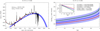 |
Fig. A.1. Fit of the source 3C 273. Other recent BH mass estimates are from Sturm et al. (2018) (Log |

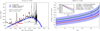 |
Fig. A.2. Fit of the source MRK 142. Other BH mass estimates are from Haas et al. (2011) (Log |

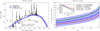 |
Fig. A.3. Fit of the source Fairall 9. |
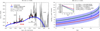 |
Fig. A.4. Fit of the source MRK 142. Spectroscopic data in the EUV region are very noisy and represented in gray to give an idea of the emission at large frequencies. Another BH mass estimate is from Li et al. (2018) (Log |
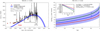 |
Fig. A.5. Fit of the source MRK 290. Spectrum rise at Log ν/Hz < 14.5 caused by the IR emission of the dusty torus. |
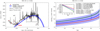 |
Fig. A.6. Fit of the source MRK 335. HST data around the Lyα-CIV region are also available, in good agreement with IUE data. The spectrum rise at Log ν/Hz < 14.4 is caused by the IR emission of the dusty torus. Other BH mass estimates are from Haas et al. (2011) (Log |
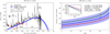 |
Fig. A.7. Fit of the source MRK 509. Spectrum rise at Log ν/Hz < 14.5 caused by the IR emission of the dusty torus. |
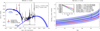 |
Fig. A.8. Fit of the source MRK 590. Prominent host-galaxy emission required in the fitting procedure. For a satisfactory fit, the AD emission has to be cut at around Log ν/Hz ∼ 15 (i.e., the AD size is smaller than 106Rg as implemented in KERRBB). In the range Log ν/Hz = 14.9 − 15, the Balmer continuum can describe the rise of spectroscopic data (not represented for clarity). For this source, the peak is not visible but we used the curvature at smaller frequencies to obtain an estimate of the position. |
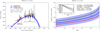 |
Fig. A.9. Fit of the source MRK 877. Some absorption features present at Log ν/Hz ∼ 15.1 − 15.2; nevertheless, they do not interfere in the fitting procedure. |
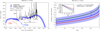 |
Fig. A.10. Fit of the source MRK 1044. The quality of spectroscopic data is low but nonetheless the fit was rather satisfactory. The Balmer continuum is shown in order to visualize the rise in the spectrum at Log ν/Hz ∼ 15. |
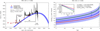 |
Fig. A.11. Fit of the source MRK 1383. |
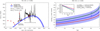 |
Fig. A.12. Fit of the source MRK 1501. Balmer continuum added to obtain a better visualization of the best fit. Spectroscopic data are not excellent (also without FUV) but are good enough to localize the spectrum peak. The other BH mass estimate shown is from Grier et al. (2017) (Log |
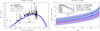 |
Fig. A.13. Fit of the source NGC 3783. Another BH mass estimate from Kollatschny & Zetzl (2013) (Log M/M⊙ = 7.47). |
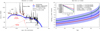 |
Fig. A.14. Fit of the source NGC 4151. Balmer continuum added to obtain a better visualization of the best fit. Spectrum rise at Log ν/Hz < 14.3 caused by the IR emission of the dusty torus. |
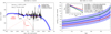 |
Fig. A.15. Fit of the source NGC 5548. Balmer continuum added to obtain a better visualization of the best fit. IUE, HST, and HUT data were smoothed in order to have a clearer spectrum. Other BH mass estimates are from De Rosa et al. (2018) (Log VP(σline)/M⊙ = 6.74 ± 0.06) and Kollatschny & Zetzl (2013) (Log M/M⊙ = 7.83). |
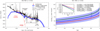 |
Fig. A.16. Fit of the source NGC 7469. Balmer continuum added to obtain a better visualization of the best fit. Spectrum rise at Log ν/Hz < 14.5 caused by the IR emission of the dusty torus. Another BH mass estimate is from Kollatschny & Zetzl (2013) (Log M/M⊙ = 7.09). |
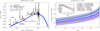 |
Fig. A.17. Fit of the source PG 0026+129. |
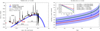 |
Fig. A.18. Fit of the source PG 0052+251. Spectrum rise at Log ν/Hz < 14.5 caused by the IR emission of the dusty torus. |
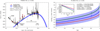 |
Fig. A.19. Fit of the source PG 0804+761. Spectrum rise at Log ν/Hz < 14.5 caused by the IR emission of the dusty torus. |
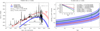 |
Fig. A.20. Fit of the source PG 0844+349. For this source, adding a galaxy template to the blue line fit or a prominent Balmer continuum does not lead to a satisfactory fit. Instead, assuming an intrinsic reddening of the source (corrected by assuming E[B − V] = 0.1 mag), the new fit (red line) describes the AGN continuum for Log ν > 14.8 (for smaller frequencies, we added the host-galaxy emission). Right panel: thick lines corresponds to the first fit (blue line on the left panel); dashed lines to the second one (red line on the left panel). |
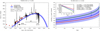 |
Fig. A.21. Fit of the source PG 0953+414. |
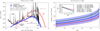 |
Fig. A.22. Fit of the source PG 1211+143. For this source, the first satisfactory fit (blue line) is given by KERRBB+host galaxy. The spectrum rise at Log ν/Hz < 14.5 is caused by the IR emission of the dusty torus. Assuming an intrinsic reddening of the source (corrected by assuming E[B − V] = 0.1 mag), the new fit (red line) describes the AGN continuum for Log ν > 14.8, with no need for the host-galaxy emission. Right panel: thick and dashed lines correspond to the first and second fits, respectively (blue and red lines on the left panel, respectively). |
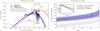 |
Fig. A.23. Fit of the source PG 1247+267. For this source, we tried to correct the spectrum emission from IGM absorption at large frequencies by following Madau (1995) and Haardt & Madau (2012). Right panel: thick and dashed lines correspond to the first and second fits, respectively (blue and red lines on the left panel, respectively). |
 |
Fig. A.24. Fit of the source PG 1307+085. |
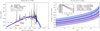 |
Fig. A.25. Fit of the source PG 1411+442. Some intrinsic absorption is present in the data but does not affect the fit. |
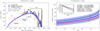 |
Fig. A.26. Fit of the source PG 1700+518. The quality of spectroscopic data at large frequencies is low; we predicted a mass larger by a factor of ∼10 with respect to RM and SE. Dust absorption could be the cause of the decreasing flux at Log ν/Hz > 15. We added the galaxy emission to the fit in order to obtain a better description of the optical continuum. |
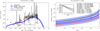 |
Fig. A.27. Fit of the source PF 2130+099. Another BH mass estimate from Grier et al. (2017) (Log |
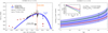 |
Fig. A.28. Fit of the source S5 0836+71. Also for this source, we tried to correct photometric data from IGM absorption at large frequencies by following Madau (1995) and Haardt & Madau (2012); new data (blue dots) are consistent with the best fit. |
Appendix B: KERRBB equations
The relativistic model KERRBB (Li et al. 2005) describes the emission produced by a thin disk around a Kerr BH. The authors included all relativistic effects such as frame-dragging, gravitational redshift, Doppler beaming and light bending. C18 build an analytic approximation of the KERRBB disk emission features considering a hardening factor equal to 1, no limb-darkening effect, and including the self-irradiation: in the case of a face-on disk, C18 found analytic expressions to compute the BH mass M and accretion rate Ṁ by fitting a given SED for different spin values. The spectrum peak νp and luminosity νpLνp are
![Mathematical equation: $$ \begin{aligned}&\frac{\nu _{\rm p}}{\text{[Hz]}} = \mathcal{A} \left[ \frac{\dot{M}}{M_{\odot , \text{ yr}^{-1}}} \right]^{1/4} \left[\frac{M}{10^9\,M_{\odot }} \right]^{-1/2} g_{\rm 1}(a, \theta _{\rm v}), \end{aligned} $$](/articles/aa/full_html/2020/08/aa36218-19/aa36218-19-eq184.gif) (B.1)
(B.1)
![Mathematical equation: $$ \begin{aligned}&\frac{\nu _{\rm p} L_{\nu _{\rm p}}}{[\mathrm{erg}\,\mathrm{s}^{-1}]} = \mathcal{B} \left[ \frac{\dot{M}}{M_{\odot , \text{ yr}^{-1}}} \right] \cos \theta _v\ g_{\rm 2}(a, \theta _{\rm v}), \end{aligned} $$](/articles/aa/full_html/2020/08/aa36218-19/aa36218-19-eq185.gif) (B.2)
(B.2)
where Log 𝒜 = 15.25, Log ℬ = 45.66, and g1, 2 is a function depending on the viewing angle of the system θv with respect to our line of sight and the BH spin a, containing all the relativistic modifications. The observed disk luminosity is  , where η is the disk spin-dependent radiative efficiency and ℱ depends on the BH spin and the viewing angle10. ℱ, and g1, 2 have an analytical form reported in C18 and C19. From Eqs. (B.1) and (B.2), the BH mass and the Eddington ratio (defined as λEdd = ηṀc2/𝒞(M/M⊙), where 𝒞 = 1.26 × 1038 erg s−1) are:
![Mathematical equation: $$ \begin{aligned} \frac{M}{M_{\odot }}&= \mathcal{D} \ \frac{[g_{\rm 1}(a, \theta _{\rm v})]^2}{\sqrt{\cos \theta _{\rm v}\ g_{\rm 2}(a, \theta _{\rm v})}}\ \frac{\sqrt{\nu _{\rm p} L_{\nu _{\rm p}}}}{\nu ^2_{\rm \mathrm{p}}}, \end{aligned} $$](/articles/aa/full_html/2020/08/aa36218-19/aa36218-19-eq187.gif) (B.3)
(B.3)
 (B.4)
(B.4)
where Log 𝒟 = 16.67 and Log ℰ = −53.675.
Appendix C: Comparison with other AD models
C.1. Shakura and Sunyaev
The most simple AD model is the one described by Shakura and Sunyaev (Shakura & Sunyaev 1973) which refers to an optically thick and geometrically thin disk around a SMBH without relativistic effects. The overall spectrum shape is similar to the KERRBB one and, as shown in Calderone et al. (2013), C18 and C19, assuming the same peak position, the Shakura and Sunyaev model corresponds to a particular KERRBB solution with a precise spin value (e.g., Fig. 3 in C19).
C.2. SLIMBH
As noted before, for very luminous QSOs the thin disk approximation breaks down due to the non-negligible disk vertical structure, and KERRBB results are no longer trustworthy. Another relativistic thin AD model is SLIMBH (Abramowicz et al. 1988; Sadowski 2009; Sadowski et al. 2009, 2011) which accounts for the vertical structure of the disk and more appropriate for bright disks (e.g., see Koratkar & Blaes 1999). Given the similarity in shape of the two models, C19 showed that, for a fixed spectrum peak position, the differences between the two models (in terms of BH masses and Eddington ratios) are less than a factor of ∼1.2 (see Figs. 3 and 4 in C19).
C.3. AGNSED
Koratkar & Blaes (1999) discussed several issues related to the black body-like AD models for AGNs: one of those is related to the soft X-ray excess observed in many objects and described by modeling an X-ray corona above the disk which scatters part of its radiation.
The AGNSED model (KD 18) is a relativistic model that describes the SED of AGNs by also taking into account the contribution of a X-ray corona located above the disk. The authors followed Novikov & Thorne (1973) to describe the AD emission: relativistic effects as the ones implemented in KERRBB (e.g., gravitational redshift, light bending, self-irradiation) are not included even though they may have a significant effect on both the disk and the X-ray corona emissions; however, for low spin values, those effects should have a minor weight on the results, especially for small viewing angles.
In order to compare the BH masses inferred with such a model and those estimated with KERRBB, we used the sources NGC 5548 and MRK 509, both present in KD 18 and our sample.
In KD 18, the authors fitted the UV-X SED of those sources assuming a viewing angle θv = 45° (the other parameters of the model are listed in their Table 2, assuming an outer disc emission). As in KERRBB, AGNSED is degenerate and by changing some of its parameters (i.e., BH mass, spin, Eddington ratio, corona size) appropriately, it is possible to reproduce the same SED (see Figs. C.1 and C.2).
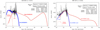 |
Fig. C.1. SED modeling of the sources NGC 5548 (left panel) and MRK 509 (right panel). The red line is the modeling of KD 18 (disk + Corona) and the blue line is the modeling adopted in this work (disk + Galaxy). As KERRBB, the AGNSED modeling is degenerate and by changing some of its parameters (i.e., BH mass, spin, Eddington ratio, X-ray corona size) appropriately, it is possible to reproduce the same SED (keeping the corona slopes constant as reported in KD 18): on the plot, we report some AGNSED BH mass solutions (in solar masses) for different spin values, along with the spectrum peak position (frequency and luminosity, in Hz and erg s−1 respectively). |
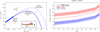 |
Fig. C.2. Left panel: scheme used to explain the difference between KERRBB and AGNSED results. The observed AD luminosity is dimmer than the intrinsic one by a factor α because a compact corona (located in the innermost part of the disk) scatters part of the disk radiation (C). The optical part of the disk (A, i.e., the emission produced by the most distant annuli of the AD) is fixed because the corona does not cover its radiation. The intrinsic disk emission can be approximately reconstructed by taking into account the factor α and by fixing the low-frequency emission; the peak of the emission (B) is produced by the AD parts closer to the corona. Right panel: comparison between AGNSED BH mass solutions (thick lines) as a function of the spin, and KERRBB ones (dashed lines) for NGC 5548 (blue) and MRK 509 (red). All these solutions describe the same SED plotted in Fig. C.1 for θv = 45°. For NGC 5548, the results of both models are consistent while for MRK 509, masses differ by a factor ≲0.2 dex. The shaded area represents the uncertainty of ∼0.1 dex (on average) linked to the spectrum peak position (see Sect. 5.1). |
Figure C.2 (right panel) shows the comparison between the BH mass estimates from KERRBB and AGNSED as a function of the BH spin: for NGC 5548, results from both models are compatible while for MRK 509, KERRBB BH masses are larger than the ones found with AGNSED by a factor ≲0.2 dex. We argue that for NGC 5548 the absence of relativistic effects in AGNSED is balanced out by modeling a large corona above the AD, leading to the same BH mass. Instead, for MRK 509, the smaller X-ray corona leads to different results because it does not compensate the differences between the two models.
If KERRBB disk luminosity is corrected from the corona coverage, then the same value of the BH mass can be found with both models. We tested this possibility by considering this simple approach: we assumed that the observed disk luminosity  (and so νpLνp) is dimmer than the intrinsic one
  by a factor α < 1: this means that (1 − α) of the disk radiation is scattered by the corona (i.e., the inner disk does not contribute to the observed emission; see Fig. C.2 left panel); assuming that the corona has a compact structure, the optical part of the spectrum produced by the outer part of the disk must not change due to the scattering and must keep the same luminosity.
We find the corrected spectrum luminosity νp, αLν, α and frequency νp, α by taking into account the correction factor α and by keeping the same luminosity at lower frequencies:
 (C.1)
(C.1)
where the exponent is derived assuming that the luminosity at Log ν ≲ 14.8 is constant11.
The factor α mimics the actual correction of the disk inner emission when this latter is cut at a certain distance from the SMBH: using the relativistic AD model described by Novikov & Thorne (1973), as an example, we considered the case with a non-spinning BH where the disk inner boundary is set to 20Rg (where Rg = GM/c2 is the gravitational radius), similar to the corona size adopted by KD 18 for MRK 509; we found that the disk peak frequency and luminosity are reduced by a factor of ∼0.14 and ∼0.17 dex, respectively; such corrections can be found for α ∼ 0.7. From Eq. (C.1), the corrected mass is smaller by factor ∼α.
Assuming that the corona scatters ≲30% of the disk radiation (e.g., Sazonov et al. 2012; Lusso & Risaliti 2017), the BH mass is reduced by a factor ≲0.15 dex. We find that, for MRK 509, a correction with α ∼ 0.7 is needed in order to make KERRBB results compatible with those found with AGNSED, while for NGC 5548, no correction is necessary because the results of both models are already compatible (see Fig. C.2).
This simple analysis showed that both models are partially consistent even though the physical background is different. Nonetheless, despite the rather good results obtained with the α correction, we warn the reader about these findings: additional uncertainties (e.g., corona geometry and size) could play an important role in estimating BH masses. Moreover, even without any correction, compatibility between the results from KERRBB, RM (SE) is still rather good (Fig. 4).
All Tables
Public spectroscopic data for the sources of our sample (collected in the online Mikulski Archive for Space Telescopes – MAST).
All Figures
|
Fig. 1. Example of a fit of the composite FUSE – HST – KPNO spectrum of the source PG 0953+414 (from Shang et al. 2005). The modeling performed with KERRBB (thick blue line) describes the AGN continuum, the iron complex (purple line), the Balmer continuum (purple dashed line), and some prominent emission lines (MgII, CIII, CIV, SiIV, Lyα) described by a simple Gaussian profile (blue lines). The red line represents the sum of all these components. The green dashed line is a standard power-law continuum (slope α = −1.77): for λ > 1300 Å, the KERRBB model overlaps the power-law rather well within the average confidence interval (∼0.05 dex, blue shaded area) and is not affected significantly by the presence of lines or other spectral features. Abundant interstellar absorption lines at λ < 1000 Å have a negligible effect on the determination of the spectral peak emission (see Sect. 4). |
| In the text | |
|
Fig. 2. Comparison between KERRBB BH mass estimates MBH, fit (inferred from the SED fitting procedure; each dot corresponds to the mean value computed using the extreme estimates given by the uncertainties) and the VPs calculated using the Hβ velocity dispersion σline (left panel) and the FWHM (right panel). We averaged all the VPs computed using data from different authors (see Table A.2; PG 1247+267 and S5 0836+71 are marked with green dots). The blue shaded area corresponds to the set of best fits between MBH, Fit and VP after considering all possible spin values between 0 and 0.998 (equations in blue on the plot are the two extreme cases; the uncertainty on the slope is ∼20%). Assuming that Log MBH, fit = LogVP + Log f, we found the scale factor f, labeled on the plot in red for the two extreme spin values. Uncertainty bars in both plots are ∼0.45 dex and ∼0.5 dex for MBH, fit and VPs respectively, and the black dashed line is the 1:1 line. |
| In the text | |
|
Fig. 3. Comparison between the KERRBB BH mass estimates MBH, fit (inferred from the SED fitting procedure) and the SE BH masses MBH, SE computed using the equation of Vestergaard & Peterson (2006) and the Hβ line (we excluded the two high-redshift sources, PG 1247+267 and S5 0836+71, for which we only have information on the CIV line; see Table A.2). The blue shaded area, the dashed black line, the reported labels, and the uncertainty bars are the same as in Fig. 2. |
| In the text | |
|
Fig. 4. Comparison between the BH masses computed from the SED fitting procedure with KERRBB (blue) and the SE (orange) and RM estimates (red, inferred with σline and a geometrical factor fBLR = 2.8 − 5.5, Graham et al. 2011top panel and Onken et al. 2004bottom panel). The average uncertainty for all the measurements is ∼0.5 dex (the results related to each source are plotted in the same order as listed in the Tables of Appendix A). |
| In the text | |
|
Fig. 5. Geometrical factor fBLR computed using Eq. (2) (e.g., Collin et al. 2006; Decarli et al. 2008) as a function of the viewing angle for different BLR thickness H/r. The blue shaded area is the scale factor range found in this work (related to VPs computed using the FWHM; see Fig. 2, right panel). The comparison leads to a range of θv and H/r consistent with the work of Mejia-Restrepo et al. (2016). |
| In the text | |
|
Fig. A.1. Fit of the source 3C 273. Other recent BH mass estimates are from Sturm et al. (2018) (Log |
| In the text | |
|
Fig. A.2. Fit of the source MRK 142. Other BH mass estimates are from Haas et al. (2011) (Log |
| In the text | |
|
Fig. A.3. Fit of the source Fairall 9. |
| In the text | |
|
Fig. A.4. Fit of the source MRK 142. Spectroscopic data in the EUV region are very noisy and represented in gray to give an idea of the emission at large frequencies. Another BH mass estimate is from Li et al. (2018) (Log |
| In the text | |
|
Fig. A.5. Fit of the source MRK 290. Spectrum rise at Log ν/Hz < 14.5 caused by the IR emission of the dusty torus. |
| In the text | |
|
Fig. A.6. Fit of the source MRK 335. HST data around the Lyα-CIV region are also available, in good agreement with IUE data. The spectrum rise at Log ν/Hz < 14.4 is caused by the IR emission of the dusty torus. Other BH mass estimates are from Haas et al. (2011) (Log |
| In the text | |
|
Fig. A.7. Fit of the source MRK 509. Spectrum rise at Log ν/Hz < 14.5 caused by the IR emission of the dusty torus. |
| In the text | |
|
Fig. A.8. Fit of the source MRK 590. Prominent host-galaxy emission required in the fitting procedure. For a satisfactory fit, the AD emission has to be cut at around Log ν/Hz ∼ 15 (i.e., the AD size is smaller than 106Rg as implemented in KERRBB). In the range Log ν/Hz = 14.9 − 15, the Balmer continuum can describe the rise of spectroscopic data (not represented for clarity). For this source, the peak is not visible but we used the curvature at smaller frequencies to obtain an estimate of the position. |
| In the text | |
|
Fig. A.9. Fit of the source MRK 877. Some absorption features present at Log ν/Hz ∼ 15.1 − 15.2; nevertheless, they do not interfere in the fitting procedure. |
| In the text | |
|
Fig. A.10. Fit of the source MRK 1044. The quality of spectroscopic data is low but nonetheless the fit was rather satisfactory. The Balmer continuum is shown in order to visualize the rise in the spectrum at Log ν/Hz ∼ 15. |
| In the text | |
|
Fig. A.11. Fit of the source MRK 1383. |
| In the text | |
|
Fig. A.12. Fit of the source MRK 1501. Balmer continuum added to obtain a better visualization of the best fit. Spectroscopic data are not excellent (also without FUV) but are good enough to localize the spectrum peak. The other BH mass estimate shown is from Grier et al. (2017) (Log |
| In the text | |
|
Fig. A.13. Fit of the source NGC 3783. Another BH mass estimate from Kollatschny & Zetzl (2013) (Log M/M⊙ = 7.47). |
| In the text | |
|
Fig. A.14. Fit of the source NGC 4151. Balmer continuum added to obtain a better visualization of the best fit. Spectrum rise at Log ν/Hz < 14.3 caused by the IR emission of the dusty torus. |
| In the text | |
|
Fig. A.15. Fit of the source NGC 5548. Balmer continuum added to obtain a better visualization of the best fit. IUE, HST, and HUT data were smoothed in order to have a clearer spectrum. Other BH mass estimates are from De Rosa et al. (2018) (Log VP(σline)/M⊙ = 6.74 ± 0.06) and Kollatschny & Zetzl (2013) (Log M/M⊙ = 7.83). |
| In the text | |
|
Fig. A.16. Fit of the source NGC 7469. Balmer continuum added to obtain a better visualization of the best fit. Spectrum rise at Log ν/Hz < 14.5 caused by the IR emission of the dusty torus. Another BH mass estimate is from Kollatschny & Zetzl (2013) (Log M/M⊙ = 7.09). |
| In the text | |
|
Fig. A.17. Fit of the source PG 0026+129. |
| In the text | |
|
Fig. A.18. Fit of the source PG 0052+251. Spectrum rise at Log ν/Hz < 14.5 caused by the IR emission of the dusty torus. |
| In the text | |
|
Fig. A.19. Fit of the source PG 0804+761. Spectrum rise at Log ν/Hz < 14.5 caused by the IR emission of the dusty torus. |
| In the text | |
|
Fig. A.20. Fit of the source PG 0844+349. For this source, adding a galaxy template to the blue line fit or a prominent Balmer continuum does not lead to a satisfactory fit. Instead, assuming an intrinsic reddening of the source (corrected by assuming E[B − V] = 0.1 mag), the new fit (red line) describes the AGN continuum for Log ν > 14.8 (for smaller frequencies, we added the host-galaxy emission). Right panel: thick lines corresponds to the first fit (blue line on the left panel); dashed lines to the second one (red line on the left panel). |
| In the text | |
|
Fig. A.21. Fit of the source PG 0953+414. |
| In the text | |
|
Fig. A.22. Fit of the source PG 1211+143. For this source, the first satisfactory fit (blue line) is given by KERRBB+host galaxy. The spectrum rise at Log ν/Hz < 14.5 is caused by the IR emission of the dusty torus. Assuming an intrinsic reddening of the source (corrected by assuming E[B − V] = 0.1 mag), the new fit (red line) describes the AGN continuum for Log ν > 14.8, with no need for the host-galaxy emission. Right panel: thick and dashed lines correspond to the first and second fits, respectively (blue and red lines on the left panel, respectively). |
| In the text | |
|
Fig. A.23. Fit of the source PG 1247+267. For this source, we tried to correct the spectrum emission from IGM absorption at large frequencies by following Madau (1995) and Haardt & Madau (2012). Right panel: thick and dashed lines correspond to the first and second fits, respectively (blue and red lines on the left panel, respectively). |
| In the text | |
|
Fig. A.24. Fit of the source PG 1307+085. |
| In the text | |
|
Fig. A.25. Fit of the source PG 1411+442. Some intrinsic absorption is present in the data but does not affect the fit. |
| In the text | |
|
Fig. A.26. Fit of the source PG 1700+518. The quality of spectroscopic data at large frequencies is low; we predicted a mass larger by a factor of ∼10 with respect to RM and SE. Dust absorption could be the cause of the decreasing flux at Log ν/Hz > 15. We added the galaxy emission to the fit in order to obtain a better description of the optical continuum. |
| In the text | |
|
Fig. A.27. Fit of the source PF 2130+099. Another BH mass estimate from Grier et al. (2017) (Log |
| In the text | |
|
Fig. A.28. Fit of the source S5 0836+71. Also for this source, we tried to correct photometric data from IGM absorption at large frequencies by following Madau (1995) and Haardt & Madau (2012); new data (blue dots) are consistent with the best fit. |
| In the text | |
|
Fig. C.1. SED modeling of the sources NGC 5548 (left panel) and MRK 509 (right panel). The red line is the modeling of KD 18 (disk + Corona) and the blue line is the modeling adopted in this work (disk + Galaxy). As KERRBB, the AGNSED modeling is degenerate and by changing some of its parameters (i.e., BH mass, spin, Eddington ratio, X-ray corona size) appropriately, it is possible to reproduce the same SED (keeping the corona slopes constant as reported in KD 18): on the plot, we report some AGNSED BH mass solutions (in solar masses) for different spin values, along with the spectrum peak position (frequency and luminosity, in Hz and erg s−1 respectively). |
| In the text | |
|
Fig. C.2. Left panel: scheme used to explain the difference between KERRBB and AGNSED results. The observed AD luminosity is dimmer than the intrinsic one by a factor α because a compact corona (located in the innermost part of the disk) scatters part of the disk radiation (C). The optical part of the disk (A, i.e., the emission produced by the most distant annuli of the AD) is fixed because the corona does not cover its radiation. The intrinsic disk emission can be approximately reconstructed by taking into account the factor α and by fixing the low-frequency emission; the peak of the emission (B) is produced by the AD parts closer to the corona. Right panel: comparison between AGNSED BH mass solutions (thick lines) as a function of the spin, and KERRBB ones (dashed lines) for NGC 5548 (blue) and MRK 509 (red). All these solutions describe the same SED plotted in Fig. C.1 for θv = 45°. For NGC 5548, the results of both models are consistent while for MRK 509, masses differ by a factor ≲0.2 dex. The shaded area represents the uncertainty of ∼0.1 dex (on average) linked to the spectrum peak position (see Sect. 5.1). |
| In the text | |
Current usage metrics show cumulative count of Article Views (full-text article views including HTML views, PDF and ePub downloads, according to the available data) and Abstracts Views on Vision4Press platform.
Data correspond to usage on the plateform after 2015. The current usage metrics is available 48-96 hours after online publication and is updated daily on week days.
Initial download of the metrics may take a while.