| Issue |
A&A
Volume 639, July 2020
|
|
|---|---|---|
| Article Number | A49 | |
| Number of page(s) | 15 | |
| Section | Planets and planetary systems | |
| DOI | https://doi.org/10.1051/0004-6361/202037644 | |
| Published online | 07 July 2020 | |
The GAPS programme at TNG
XXII. The GIARPS view of the extended helium atmosphere of HD 189733 b accounting for stellar activity★
1
Dipartimento di Fisica, Università degli Studi di Torino,
via Pietro Giuria 1,
10125
Torino, Italy
e-mail: This email address is being protected from spambots. You need JavaScript enabled to view it.
2
INAF – Osservatorio Astronomico di Capodimonte,
Salita Moiariello 16,
80131
Naples, Italy
3
INAF – Osservatorio Astrofisico di Torino,
Via Osservatorio 20,
10025
Pino Torinese, Italy
4
INAF – Osservatorio Astronomico di Brera,
Via E. Bianchi 46,
23807
Merate (LC), Italy
5
Observatoire de l’Université de Genève,
51 chemin des Maillettes,
1290
Versoix, Switzerland
6
Space Research Institute, Austrian Academy of Sciences,
Schmiedlstrasse 6,
8042
Graz, Austria
7
Thüringer Landessternwarte,
Tautenburg Sternwarte 5,
07778
Tautenburg, Germany
8
National Solar Observatory,
Tucson,
AZ
85719,
USA and Steward Observatory, University of Arizona, Tucson, AZ 85721,
USA
9
Fundación G. Galilei – INAF (Telescopio Nazionale Galileo),
Rambla J. A. Fernández Pérez 7,
38712
Breña Baja (La Palma), Spain
10
INAF – Osservatorio Astrofisico di Arcetri,
Largo E. Fermi 5,
50125
Firenze, Italy
11
Department of Physics, University of Warwick,
Gibbet Hill Road,
Coventry,
CV4 7AL, UK
12
Centre for Exoplanets and Habitability, University of Warwick,
Gibbet Hill Road,
Coventry,
CV4 7AL, UK
13
INAF – Osservatorio Astrofisico di Catania,
Via S. Sofia 78,
95123
Catania, Italy
14
INAF – Osservatorio Astronomico di Padova,
Vicolo dell’Osservatorio 5,
35122,
Padova, Italy
15
Dipartimento di Fisica G. Occhialini, Università degli Studi di Milano-Bicocca,
Piazza della Scienza 3,
20126
Milano, Italy
16
Department of Physics, University of Rome Tor Vergata,
Via della Ricerca Scientifica 1,
00133
Rome, Italy
17
Max Planck Institute for Astronomy,
Königstuhl 17,
69117
Heidelberg, Germany
18
Anton Pannekoek Institute for Astronomy, University of Amsterdam,
Science Park 904,
1098 XH
Amsterdam, The Netherlands
19
INAF – Osservatorio Astronomico di Palermo,
Piazza del Parlamento, 1,
90134
Palermo, Italy
20
INAF Osservatorio Astronomico di Trieste,
via Tiepolo 11,
34143
Trieste, Italy
21
Instituto de Astrofísica de Canarias,
C/Vía Láctea s/n,
38205
La Laguna (Tenerife), Spain
22
Departamento de Astrofísica, Univ. de La Laguna, Av. del Astrofísico Francisco Sánchez s/n,
38205
La Laguna (Tenerife), Spain
23
Astronomy Department, 96 Foss Hill Drive, Van Vleck Observatory 101, Wesleyan University,
Middletown,
CT
06459, USA
24
Centro de Astrobiología (CSIC-INTA),
Carretera de Ajalvir km 4, 28850 Torrejón de Ardoz,
Madrid, Spain
25
INAF – Osservatorio di Cagliari,
via della Scienza 5,
09047
Selargius,
CA, Italy
26
Dip. di Fisica e Astronomia Galileo Galilei, Universit‘a di Padova,
Vicolo dell’Osservatorio 2,
35122
Padova, Italy
27
Institut für Astrophysik,
Friedrich-Hund Platz 1,
37077
Göttingen, Germany
Received:
3
February
2020
Accepted:
11
May
2020
Abstract
Context. Exoplanets orbiting very close to their parent star are strongly irradiated. This can lead the upper atmospheric layers to expand and evaporate into space. The metastable helium (He I) triplet at 1083.3 nm has recently been shown to be a powerful diagnostic to probe extended and escaping exoplanetary atmospheres.
Aims. We perform high-resolution transmission spectroscopy of the transiting hot Jupiter HD 189733 b with the GIARPS (GIANO-B + HARPS-N) observing mode of the Telescopio Nazionale Galileo, taking advantage of the simultaneous optical+near infrared spectral coverage to detect He I in the planet’s extended atmosphere and to gauge the impact of stellar magnetic activity on the planetary absorption signal.
Methods. Observations were performed during five transit events of HD 189733 b. By comparison of the in-transit and out-of-transit GIANO-B observations, we computed high-resolution transmission spectra. We then used them to perform equivalent width measurements and carry out light-curves analyses in order to consistently gauge the excess in-transit absorption in correspondence with the He I triplet.
Results. We spectrally resolve the He I triplet and detect an absorption signal during all five transits. The mean in-transit absorption depth amounts to 0.75 ± 0.03% (25σ) in the core of the strongest helium triplet component. We detect night-to-night variations in the He I absorption signal likely due to the transit events occurring in the presence of stellar surface inhomogeneities. We evaluate the impact of stellar-activity pseudo-signals on the true planetary absorption using a comparative analysis of the He I 1083.3 nm (in the near-infrared) and the Hα (in the visible) lines. Using a 3D atmospheric code, we interpret the time series of the He I absorption lines in the three nights not affected by stellar contamination, which exhibit a mean in-transit absorption depth of 0.77 ± 0.04% (19σ) in full agreement with the one derived from the full dataset. In agreement with previous results, our simulations suggest that the helium layers only fill part of the Roche lobe. Observations can be explained with a thermosphere heated to ~12 000 K, expanding up to ~1.2 planetary radii, and losing ~1 g s−1 of metastable helium.
Conclusions. Our results reinforce the importance of simultaneous optical plus near infrared monitoring when performing high-resolution transmission spectroscopy of the extended and escaping atmospheres of hot planets in the presence of stellar activity.
Key words: planets and satellites: atmospheres / planets and satellites: fundamental parameters / techniques: spectroscopic / planets and satellites: individual: HD 189733 b / stars: activity
Based on observations made with the Italian Telescopio Nazionale Galileo (TNG) operated by the Fundación Galileo Galilei (FGG) of the Istituto Nazionale di Astrofisica (INAF) at the Observatorio del Roque de los Muchachos (La Palma, Canary Islands, Spain).
© ESO 2020
1 Introduction
Exoplanets that orbit very close to their host stars are subject to extreme physical processes (e.g. hydrodynamic escape). For instance, the intense X-ray and extreme ultraviolet (EUV) irradiation received from the parent stars can lead the gas content in the upper layers of their atmosphere to expand and reach high velocities. The gas fraction with a velocity greater than the escape velocity can then overcome the planetary force of gravity, escaping into space. Atmospheric evaporation processes driving strong mass loss might be responsible for the paucity of planets with intermediate mass and size (sub-Jovian) with periods ≤3 d (the so-called “Neptunian desert”; see e.g. Lecavelier Des Etangs 2007; Beaugé & Nesvorný 2013; Lundkvist et al. 2016; Mazeh et al. 2016; Owen & Lai 2018) observed in the mass(radius)-period distribution of close-in exoplanets.
Hydrogen has long been investigated as a tracer for atmospheric evaporation because it is the lightest and most abundant element in giant planets, and therefore it can easily escape and produce an extended exosphere surrounding the planet. The first observation of this effect was obtained by Vidal-Madjar et al. (2003) for the transiting hot Jupiter HD 209458 b. Based on space-borne spectroscopy carried out with the Space Telescope Imaging Spectrograph (STIS), installed on the Hubble Space Telescope (HST), strong variations in the ultraviolet Ly-α emission line at 121.567 nm between in-transit and out-of-transit spectra demonstrated the presence of an extended comet-like tail of escaping hydrogen atoms from HD 209458 b. Additional evidence for atmospheric escape in other giants has been obtained using Ly-α spectroscopy (e.g. Lecavelier Des Etangs et al. 2010, 2012; Bourrier et al. 2013, 2018; Kulow et al. 2014; Ehrenreich et al. 2015; Lavie et al. 2017).
However, this proxy is strongly affected by interstellar absorption and by geocoronal emission (due to the Earth’s exosphere). Therefore, only the wings of the Ly-α line can be used to probe escaping exoplanetary atmospheres (e.g. Ehrenreich et al. 2015).
The 1083.3 nm He I near-infrared (nIR) triplet (vacuum wavelength)1 is very weakly affected by interstellar absorption and it can be observed from the ground. It is a well-known diagnostic used in a variety of astrophysical contexts, for instance to study the structure of the solar chromosphere and transition region, prominences, flares (e.g. Andretta et al. 2008), magnetic activity in cool stars (e.g. Zarro & Zirin 1986), the dynamics of stellar winds (e.g. Dupree et al. 1992), the outflows from quasars (e.g. Leighly et al. 2011), and to trace planetary nebulae (Weidmann et al. 2013). The He I nIR triplet was first suggested to be a relevant absorption signature in the spectra of exoplanetary atmospheres by Seager & Sasselov (2000), while more recent theoretical work (Oklopčić & Hirata 2018) revisited those findings to infer good prospects for the observability of extended atmospheres of known hot planets through this channel.
Prompted by the theoretical expectations, early attempts to detect the presence of helium in the extended atmospheres of exoplanets employing medium-resolution spectroscopy (Moutou et al. 2003) only succeeded in placing upper limits on this absorption feature. However, the tide has recently turned thanks to renewed efforts carried out both at low and high spectral resolution in space and from the ground, respectively. Using the Wide Field Camera 3 (WFC3) on board HST, an excess absorption in the helium triplet was detected in the atmosphere of the two warm Neptunes, WASP-107b and HAT-P-11b (Spake et al. 2018; Mansfield et al. 2018). Using CARMENES (Calar Alto high-Resolution search for M dwarf with Exoearths with Near-infrared and optical Échelle Spectrographs) data, Nortmann et al. (2018), Allart et al. (2018, 2019), Salz et al. (2018), and Alonso-Floriano et al. (2019) confirmed the presence of extended atmospheres of helium in HAT-P-11b and WASP-107b, and reported new detections of He I absorption in HD 189733 b, WASP-69b, and HD 209458 b.
However, all excited levels of helium, including the lower level of the triplet 1083.3 nm line, the metastable level 1s 2s 3S, lie almost 20 eV above the 1s2 1S ground state. In plasmas at temperatures below a few 104 K, the level population of that state, and of all the triplet states, is usually negligible. Indeed, no He I line is produced in the photosphere of stars of spectral type later than A, which includes the majority of stars that host hot exoplanets. Thus, in contrast to the Ly-α diagnostic of atmospheric evaporation, which arises from the ground level of H I, a non-thermal process is required to populate the levels producing the observed absorption in the He I 1083.3 nm triplet.
A consensus has not yet emerged on the nature of the non-thermal processes responsible for the observed He I 1083.3 nm line strength in the outer atmosphere of the Sun and of solar-type stars. Various non-equilibrium collisional processes have been proposed (e.g. Andretta et al. 2000; MacPherson & Jordan 1999; Golding et al. 2016). As an alternative, a connection with the solar and stellar coronal emission has often been invoked. It was pointed out early on(Goldberg 1939; Hirayama 1971) that EUV radiation below 50.4 nm could photoionize neutral He atoms. Subsequent recombination cascades can then populate the triplet system, and in particular the 1s 2s 3S level. The depopulation of this triplet state (which can only radiatively decay through a forbidden-line photon) progresses slowly, 10.9 day−1 (Drake 1971), making it metastable. Atoms in that state can therefore efficiently scatter nIR photons at 1083.3 nm. The process has been described by Zirin (1975) in the context, for example, of solar and stellar chromospheres, and analysed in detail by Andretta & Jones (1997), but it can also act in exoplanet escaping atmospheres where it could produce the strong absorption feature in the transmission spectrum (Seager & Sasselov 2000).
It is therefore clear that, in the absence of sufficient EUV illumination from the host star, no absorption features from excited levels of He I in the transmission spectrum of exoplanet escaping atmospheres can be observed. Since in solar-type or cool stars such EUV radiation is only associated with stellar activity phenomena, we expect the signatures of exoplanet escaping atmospheres to be clearly observable in the He I 1083.3 nm line only in exoplanets orbiting active or moderately active stars (Oklopčić 2019). This implies that, for a correct quantitative interpretation of observed absorption in the He I 1083.3 nm line, it is imperative to obtain simultaneous estimates of the activity level of the host star.
The presence of inhomogeneities on the stellar surface can also complicate the analysis of transmission spectra in a different respect: for example, the transiting of a planetary disc over quiet stellar regions, which are regions with below-average He I absorption, can mimic a pseudo-absorption at the position of the helium triplet. Conversely, the occultation of active regions by the transiting exoplanet could produce an emission signal in the transmission spectrum that could reduce the absorption signal related to the planetary atmosphere. In their study focused on HD 189733 b, Salz et al. (2018) discussed how these pseudo-signals, which are due to stellar activity, can interfere with the atmospheric absorption signal, but without a clear evaluation of these effects and how they can be distinguished. However, the analogy with the Sun suggests that the He I 1083.3 nm line in active, solar-like stars is much more sensitive to the presence of plage-like regions or stellar prominences than to starspots. This raises the possibility that a better understanding of the relative contribution to observed helium absorption features could be gleaned by combined analyses of the He I line and other activity-sensitive spectral diagnostics.
In this paper we present a new investigation of the extended atmosphere of the hot Jupiter HD 189733 b at high spectral resolution both in the optical and nIR using simultaneous observations gathered with the GIANO-B and the High Accuracy Radial velocity Planet Searcher for the Northern emisphere (HARPS-N) spectrographs (Sect. 2). We employ a multi-technique approach to confirm the recent detection of helium in the planet’s extended atmosphere (Sect. 3), and describe a new methodology to consistently evaluate the impact of stellar activity pseudo-signals on the true absorption by circumplanetary material (Sect. 4). We then interpret the helium absorption observations that are not significantly affected by stellar contamination in terms of effective mass loss, using detailed 3D simulations of the atmosphere of HD 189733 b (Sect. 5). Finally, we summarize our results and conclude (Sect. 6) by highlighting possible future applications of this method to put more constraints on real planetary absorption.
HD 189733 b GIARPS observations log.
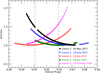 |
Fig. 1 Airmass during the GIARPS observations. The colour and symbol coding presented here will be adopted consistently throughout the work. The contact points t1 and t4 are marked with vertical dashed lines. |
2 Observations
We observed the system HD 189733 using the GIANO-B + HARPS-N (GIARPS) observing mode of the Telescopio Nazionale Galileo (TNG) telescope (Claudi et al. 2017), which, by obtaining high-resolution spectra with the HARPS-N (resolving power R ~115 000) and GIANO-B (R ~ 50 000) spectrographs, allows for simultaneous coverage over the optical (0.39–0.69 μm for HARPS-N) and nIR (& 0.95–2.45 μm for GIANO-B) wavelength ranges. The full dataset encompasses a total of five primary transit events of HD 189733 b, three observed on UT 30 May 2017, UT 20 July 2017, and UT 18 October 2018, within the context of the Global Architecture of Planetary Systems (GAPS). Project, and two scheduled on UT 19 June 2017 and UT 9 July 2017 as part of programme AOT35_14 (P.I.: V. Andretta). A log of the observations with the number of collected spectra, exposure times, and achieved signal-to-noise ratio (S/N) is given in Table 1. The target was observed at airmass as low as 1.005 and as high as 2.004 (Fig. 1). Table 2 lists the system parameters adopted in this work.
Stellar and planetary parameters adopted in this work.
2.1 GIANO-B data
In order to be operated in GIARPS mode, the nIR high-resolution spectrograph GIANO (Oliva et al. 2006) was recently moved at the Nasmyth-B focal station of the TNG (Carleo et al. 2018), and re-named GIANO-B. The GIANO-B echellogram has a fixed format and includes 50 orders. The spectra are imaged on a HAWAII-2 2048 × 2048 detector. The data consist of a sequence of nodded observations, with the target observed at predefined A and B positions on the slit, following an ABAB pattern (Claudi et al. 2017). For each nodding sequence, the thermal background and telluric emission lines are monitored at the slit position that is not illuminated by the target, and are subsequently subtracted. The GIANO-B spectra are extracted, blaze corrected, and wavelength calibrated using the GOFIO data reduction pipeline (Rainer et al. 2018).
2.2 HARPS-N data
HARPS-N is the high-resolution, fibre-fed, cross-dispersed echelle spectrograph mounted at the Nasmyth-B focus of the TNG (Cosentino et al. 2012). The observations were carried out using the objAB observational setup, with fibre A on the target and fibre B on the sky. The fibre entrance is reimaged onto a 4k × 4k charge-coupled device (CCD), where echelle spectra of 69 orders are formed for each fibre. The HARPS-N data are reduced with the standard Data Reduction Software (DRS), version 3.7 (DRS, Cosentino et al. 2012).
3 Data analysis of the He I 1083.3 nm triplet
In the following section we discuss the steps we perform to analyse the He I 1083.3 nm triplet.
3.1 Further treatment of GIANO-B data
For the purpose of our scientific analysis, the GIANO-B spectra reduced by the GOFIO pipeline require additional processing steps, as follows.
3.1.1 Wavelength calibration refinement
Temporal variations in the wavelength solution due to a non-optimal stability of the GIANO-B spectrograph are removed using the approach described in Brogi et al. (2018), which is based on a spline interpolation procedure. The initial wavelength calibration, obtained using an U-Ne lamp, is then refined employing a telluric spectrum as in Brogi et al. (2018). The magnitude of these wavelength calibration refinements, for the considered nights and in the region around the He I triplet, is ~1.3 km s−1, lower than an individual GIANO-B resolution element (1 pixel = 2.7 km s−1).
3.1.2 Telluric lines removal
When working with ground-based spectra, we must take into account that they are contaminated by the imprints of the Earth’s atmosphere. Therefore, our data must be corrected by removing telluric features. First of all, for each night, we normalize the spectra by dividing them by the average flux computed in two intervals on the blue (1082.6–1082.8 nm) and red (1083.9–1084.0 nm) sides of the He I triplet lines. To take into account possible variations between the two nodding positions, the spectra acquired in nodding position A (A-spectra) are treated separately from those acquired in position B (B-spectra). In order to recognize and remove the telluric contamination, we follow the methods implemented by Snellen et al. (2008), Vidal-Madjar et al. (2010), and Astudillo-Defru & Rojo (2013). These techniques consider that the logarithm of the strength of the telluric lines increases linearly with the airmass. This is a consequence of the solution of the radiative transfer equation assuming only absorption. The total intensity at a certain wavelength I0λ, reaching the top of the atmosphere, is converted into an observed spectrum Iλ according tothe formula (Vidal-Madjar et al. 2010)
 (1)
(1)
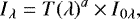
where T(λ) is the vertical atmospheric transmittance (the telluric spectrum) and a is the airmass. For each night and nodding position, we derive T(λ), modelling the relationship in Eq. (1) via linear regression (Wyttenbach et al. 2015). This operation is performed using only the out-of-transit spectra because during transit the presence of the planetary atmosphere could leave detectable imprints in Iλ. The only exception is transit 2 for which, due to the lack of a sufficient number of observations before the transit, we also have to use the in-transit spectra to compute a high-quality telluric spectrum (see e.g. Wyttenbach et al. 2015). In Fig. 2 we show the telluric spectrum built for the night with the highest S/N (20 July 2017) considering only the A-spectra. This is consistent with the telluric spectrum generated via the ESO Sky Model Calculator2.
Each stellar spectrum is then corrected from telluric contamination by dividing it by  . We note that some strong telluric features are not fully removed. This might be due to either short timescale variations in telluric species content or second-order deviations from the linear dependence on the airmass (Astudillo-Defru & Rojo 2013). However, since these telluric residuals do not fall into the wavelength ranges used in the presented analysis, our results are not affected.
Generally, observations from the ground are also contaminated by telluric emission lines. In particular, in the spectral region of interest, there are three OH emission lines that fall near the He I triplet (more precisely at λ 1083.21 nm, λ 1083.24 nm, and λ 1083.43 nm). However, as the GIANO-B observations are acquired with a nodding pattern that allows for substraction of the thermal background and emission lines at the level of the standard data extraction pipeline (see Sect. 2.1), at this stage of the analysis we no longer need to manually correct for the OH lines, as has been done in other works (e.g. Salz et al. 2018; Allart et al. 2019; Nortmann et al. 2018).
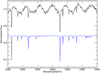 |
Fig. 2 Telluric absorptions spectrum built for the highest S/N night considering only the GIANO-B A-spectra. As a comparison,the telluric spectrum generated via the ESO SKy Model Calculator is shown in blue with an offset of −0.3. The two spectra are consistent. In our telluric spectrum the fringing pattern affecting GIANO-B spectra is also visible. |
3.1.3 Fringing correction
The telluric spectrum in Fig. 2 clearly shows a sinusoidal fringing pattern, which is known to affect high S/N GIANO-B spectra in the central and red part of the blue orders3. The effect is caused by the sapphire substrate (~0.38 mm thick) placed above the sensitive part of the detector which, behaving like a Fabry-Pérot, generates interference fringing with a peak-to-peak distance approximately equal to 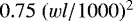 nm, where wl is the wavelength expressed in nanometres. Such fringing patterns must be corrected for if we want to study the He I triplet. In this work, we mitigate fringing effects by adopting two different approaches, one implemented at the level of the original spectra (Sect. 4.3), and the second when working with the transmission spectra (Sects. 3.2 and 3.3). In Appendix A we discuss the impact of these two techniques on the determination of the He I absorption levels.
The GIANO-B spectra, subjected to wavelength calibration refinement and telluric line removal, are then used to investigate the extended atmosphere of HD 189733 b, searching for planetary helium absorption in correspondence with the 1083.3 nm triplet using a multi-technique approach: transmission spectroscopy and tomography, transmission spectra equivalent widths, and light-curve analysis.
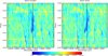 |
Fig. 3 Transmission spectra shown in tomography in the planetary (left) and stellar (right) rest frame, as a function of the wavelength and the orbital phase (transmission spectra are binned both in wavelength and in phase). An excess absorption (in blue) is present during the transit, the three helium triplet lines are indicated with vertical black lines. The contact point t1, t2, t3 and t4 are marked with horizontal white lines. |
3.2 Transmission spectroscopy and tomography
When the planet passes in front of its host star, a transmission spectrum can be measured. This represents the fractional area of the stellar disc covered by the planetary atmosphere as a function of wavelength, and can used to investigate the optically thin regions of the planetary atmosphere. We compute transmission spectra as follows. The telluric-corrected GIANO-B spectra are initially shifted into the stellar rest frame by accounting for the barycentric Earth radial velocity, the stellar reflex motion induced by the planet, and the systemic velocity. Then, by averaging the out-of-transit A-spectra (B-spectra), a master-out spectrum MA (MB) is created. All the A-spectra (B-spectra) are successively divided by MA (MB) to create the transmissionspectra TA (TB), which are then corrected for fringing effects using Method #1 described in Appendix A.
The two panels of Fig. 3 show a two-dimensional map of the full time series of the fringing-corrected transmission spectra of HD 189733 b in wavelength-orbital phase space in the neighbourhood of the He I triplet lines. The tomographic representation is routinely used to highlight the true reference frame of each absorption and emission signal (e.g. Borsa & Zannoni 2018). When applying the tomography in the stellar reference frame (right panel of Fig. 3), during the transit an excess of absorption is clearly present at the position of the stellar helium lines. The signal follows the planetary radial velocity, revealing its planetary origin4. At this point, we shift the transmission spectra in the planetary rest frame (left panel of Fig. 3) and, for the two nodding positions, we build a mean transmission spectrum using the average of the TA (TB) between the second (t2) and the third (t3) contact points. Then, for every night, by averaging these two mean transmission spectra we obtain a single master transmission spectrum TAB. The mean TAB of the five observed transits is shown in Fig. 4. We clearly identify an absorption feature with a full width half maximum = 0.091 ± 0.005 nm. The peak of the excess absorption is measured to be 0.75 ± 0.03% (25σ), evaluated by fitting a Gaussian (with a local non-linear least-squares method based on the Levenberg-Marquardt algorithm) in the core of the strongest He I component. The measured absorption levels in individual nights are shown in Table 3. We note that the helium feature has a net blueshift of − 3.0 ± 0.6 km s−1. This is in agreement with the findings by Salz et al. (2018), who reported a blueshift of − 3.5 ± 0.4 km s−1.
Figure 3 highlights that the helium transmission signal seems to start after t1, and close to t2. This is compatible with an extended atmosphere with a compact structure, meaning the helium atmosphere is not so elongated as already to give a signal at first contact, but it becomes detectable when the planet is completely inside the stellar disc. This is in agreement with the results of our 3D simulations (see Sect. 5) and with findings by Salz et al. (2018).
Average peak absorption in the strongest He I component in each individual night.
3.3 Transmission spectra equivalent widths and light-curve analysis
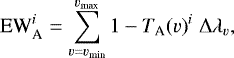
Once the series of TA and TB have been computed, we evaluate the excess in-transit absorption in the helium triplet lines by using the methodology proposed by Cauley et al. (2015, 2016, 2017a,b), and Yan & Henning (2018) for the analysis of the Balmer lines. For every night, the absorption is calculated as the equivalent width of the transmission spectrum at the position of the helium line,
 (2)
(2)
where  is the equivalent width corresponding to the transmission spectrum
  , at the orbital phase i, for the nodding position A, and Δλv is the wavelength difference atvelocity v. We then compute
  in a similar way for nodding position B. We measure the absorption of the helium triplet across a 40 km s−1 band, from − 20 km s−1 (λmin ~1083.22 nm) to + 20 km s−1 (λmax ~1083.36 nm), centred on the strongest component of the triplet. The interval is chosen to avoid possible contamination from the nearby telluric line at 1083.51 nm.
All the five nights exhibit an extra absorption during the transit, while the out-of-transit EW values are compatible with zero. The mean in-transit He I extra absorption due to the extended planetary atmosphere, calculated by merging the two nodding positions and averaging the EW values between contact points t2 and t3, is  , which corresponds to a 11σ detection (the error bar on this value is evaluated as the standard deviation of the mean).
Starting from the TA (TB) shifted into the planetary rest frame, for each night we subsequently compute a light curve of the He I lines as a function of time (e.g. Charbonneau et al. 2002; Snellen et al. 2008). For every orbital phase, we average the corresponding TA (TB) over a velocity range from –20 to +20 km s−1 centred on the strongest He I component, analogously to the equivalent width method. In Fig. 5 we show the derived light curves binned into intervals of 0.005 in phase. Table 4lists the average nightly He I transit depths in the light curves calculated between contact points t2 and t3.
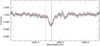 |
Fig. 4 Mean TAB of the five observed nights in the planetary rest frame. We detect an average absorption signal of 0.75 ± 0.03% (25σ) in the strongest component of the helium triplet. A Gaussian fit is shown as the red line. Vertical dashed lines indicate the three helium triplet lines. |
Averaged He I transit depths in each individual night between contact points t2 and t3 in the transmission light curves.
4 Planetary absorption versus stellar activity effects
Our multi-technique analysis of the GIANO-B transmission spectra of HD 189733 b confirms the absorption feature at the wavelength of the He I nIR triplet. By looking at the tomography map, we have shown that the signal is at rest in the planetary reference frame, and by using different approaches (i.e. transmission-spectra equivalent-widths technique and light-curve analysis) we have shown that the signal is present in all five transits. The strength of the average absorption signal is measured to be slightly lower (a 2.6σ difference) than that (0.88 ± 0.04%) reported by Salz et al. (2018) in their analysis of CARMENES primary transit spectra of HD 189733 b. However, by looking at the left panel of Fig. 5 and Table 4, the night-to-night variability of the He I absorption levels appears rather clear (a 3.3σ and 4σ departure for night 1 and 3, respectively, with respect to the quasi-constant values for the other three nights).
A likely origin for this variability could be the planetary transit on an inhomogeneous stellar surface. The occultation of active and quiescent regions by the transiting planet can indeed alter the planetary helium absorption signal. The effect on high-resolution transit signatures seen in chromospheric lines is sometimes referred to as the “contrast effect”, and has been extensively studied in the case of HD 189733b, for instance by Barnes et al. (2016) and Cauley et al. (2017a, 2018). The latter paper, in particular, discusses the contrast effect for several chromospheric lines in addition to the He I line.
4.1 Fractional area of active regions on HD 189733
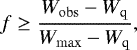
The contrast effect on the transit signal clearly depends on the type and extent of non-quiescent (active) regions on the stellar surface. Following Andretta & Giampapa (1995) and assuming that the active regions are similar to solar plage regions, it is possible to obtain a lower limit for the active region area coverage, f, through a measurement of the equivalent width of the stellar He I 1083.3 nm line alone, using the relation
 (3)
(3)
where Wq is the intrinsic equivalent width in the quiescent region, Wmax is the maximum intrinsic equivalent width in the active region, and Wobs is the observed equivalent width of the line5. We measure the equivalent widths for the off-transit He I profiles for all the transit dates by means of multi-line fits including the three components of the helium triplet and the main stellar and telluric blends, as discussed by Andretta et al. (2017). We obtain values for Wobs ranging from 320 to 350 mÅ. Adopting the values Wq = 40 mÅ and Wmax = 410 mÅ given by Andretta et al. (2017), we therefore estimate that at least 75% of the stellar surface of HD 189733 is covered by plage-like active regions. A better estimate of the fractional active region coverage could be obtained by additionally measuring the He I 587.6 nm line (observed in the HARPS-N range) and computing the He I 1083.3 nm and 587.6 nm intrinsic equivalent widths from active regions; in the case of HD 189733 this would be over a grid of non-local thermodynamic equilibrium (NLTE) radiative transfer calculations. Such calculations are outside the scope of this work, although we do plan to include them in a follow-up analysis.
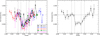 |
Fig. 5 Left panel: transmission light curve of the He I lines in the planetary rest frame from the five transits. Contact points t1, t2, t3, and t4 are marked with vertical dashed lines. Right panel: transmission light curve, binned in phase, obtained for the five nights combined. Contact points t1, t2, t3, and t4 are marked with dashed lines. The continuum behaviour is indicated by the horizontal dashed line. |
4.2 Signature of the contrast effect in chromospheric lines
Here we follow instead a different approach; we look for signatures of the contrast effect in other chromospheric lines in addition to the He I lines. One of the most prominent chromospheric lines in our dataset is the Hα 656.3 nm line. To illustrate the different effect of stellar surface inhomogeneities on the He I and the Hα lines. In Fig. 6 we show a typical solar image of central line intensity in the two lines. The He I 1083.3 nm map was obtained from the File Transfer Protocol (FTP) archive of the National Solar Observatory Integrated Synoptic Program (NISP6). The near simultaneous H I 656.3 nm map is from the Kanzelhöhe Observatory and was obtained from the FTP site of the Big Bear Solar Observatory FTP archive of the Global Hα Network7. Those maps clearly show that plage-like active regions appear darker than the rest of the stellar disc in He I, and brighter in Hα. We also note that, on the other hand, filaments appear darker in both lines. This is typical behaviour of those lines in the Sun and, by extension, in solar-like active stars such as HD 189733.
Considering the He I line alone, a planet transiting over quiescent areas of the star would increase the weight of active regions in the observed flux, thus producing a stronger 1083.3 nm absorption. Viceversa, if the planet occults an active region, the net effect is a reduced He I absorption. These variations induced by the contrast effect in thein-transit spectrophotometry are very difficult to distinguish from the intrinsic signal due to the planet atmosphere. Salz et al. (2018) tried to distinguish between these two contributions but did not obtain clear results.
On the other hand, the signal perturbations in the Hα line due to the contrast effect have an opposite sign: when the planet occults quiescent regions, the total flux in the line increases, while occultation of active regions produces a decrease of the line flux (assuming that the dominant inhomogeneities are plage-like regions). We also note that the other prominent chromospheric lines in the HARPS-N range, the Na I D doublet at 589.6 nm (D1) and 589.0 nm (D2), behave very much like the Hα line (e.g. Cauley et al. 2018).
Therefore, if we find evidence that the perturbations in the He I 1083.3 nm and the Hα signals are anti-correlated, we could reasonably infer that the source of the signal is due to the contrast effect. For this reason, we performed a comparative analysis with the Hα line to determine the extent to which our He I planetary detection is contaminated by stellar activity, first analysing the out-of-transit line profiles, then the perturbations during the transit of HD 189733b.
4.3 Stellar variability across different nights
In order to estimate the role of stellar activity in the observed He I transit signal, we analyse the average stellar spectra outside the transit as a function of stellar activity. In the case of GIANO-B data, we remove the fringing pattern around the He I line using Method #2 described in Appendix A. We do not attempt to correct the line profiles for the telluric spectrum.
We first measure the  index from HARPS-N spectra. The average values for each night are given in Table 5. From those values, it is clear there is a noticeable variability in stellar activity, with the star being in its higher activity state during transit 1, while transits 3 and 4 exhibit similar but lower levels of activity. The activity of HD 189733 is lowest during transits 2 and 5. We also measure the
  index for each HARPS-N spectrum, thus obtaining temporal sequences of that index. Inspection of those light curves does not reveal significant events such as flares. The variations observed during each night are of lower amplitude than the variations of the night-to-night average value given in Table 5.
For each transit date, we then compute the average out-of-transit profile of several lines sensitive to stellar chromospheric activity: Hα, Na I D1 and D2, Ca II H and K (all from HARPS-N), and He I 1083.3 nm (from GIANO-B). Each average line profile is normalized using the wings of theline or the nearby continuum (Fig. 7, top panels). It should be noted that the integrated  indices listed in Table 5 are mean values for each transit night, while the average profiles shown in Fig. 7 are computed from out-of-transit spectra only.
From the set of five average out-of-transit profiles, Fi(λ) (i =1…5), we compute an average reference line profile, Fref(λ). In the bottom panels of Fig. 7 we show the variation of line fluxes with respect to that reference profile: Ri (λ) = Fi(λ)∕Fref(λ). We only show the Na I D1 line since the D2 line is significantly affected by telluric absorption on some dates. Also, the Ca II K and H lines behave very similarly, thus we only show the latter. We notice above all that the relative variations of He I fluxes are anti-correlated with Hα and Ca II H: for example when Hα displays an excess flux in the line core (as in the profile from transit 1), the helium line shows a deeper core flux. The Na I D1 relative flux, although noisier and narrower, follows the trend of the Hα line, as expected from the analogy with solar observations and in qualitative agreement with the calculations of Cauley et al. (2018).
To better quantify this effect, we estimate the peak values of Ri (λ) in the line core by a Gaussian fit in a range as free as possible from telluric blends. More specifically, the ranges for the fit procedure are: 656.177–656.345 nm for Hα, 1083.23–1083.38 nm for He I 1083.3 nm, and 589.57–589.60 nm for Na I D1. The resulting peak values of Ri(λ) are shown in Fig. 8 as a function of the activity index  .
.
As a sanity check, we also estimate the peak value of Ri (λ) in the core of the Ca II H line, within the range 396.82–396.87 nm, but we do not display the results in Fig. 8 because they are very well correlated with  , as expected (correlation coefficient: 0.98). The correlation coefficients with
  for the other lines are tabulated in Table 6 along with their p-values. We also compute the linear fit of the relative variation of line depth with
  (dashed lines in Fig. 8). The slopes of the fit are also given in Table 6. If we interpret these values as the line sensitivity to activity, we can say that, in absolute terms, He I 1083.3 nm and Na I D1 have similar sensitivity to
  , while Hα is roughly twice as sensitive as both of them.
We notice in particular that there is an excellent positive correlation between variations in the Hα line depth with activity. A good correlation, but of opposite sign, is seen in the He I 1083.3 nm too. Once more, the Na I D1 variations behave like the Hα line, although the data point for the most active night (transit 1) deviates from the linear trend seen in the other four nights.
From this analysis, we conclude that the observed night-to-night variations of out-of-transit average profiles are consistent with the picture of a stellar surface covered by large plage-like active regions producing an anti-correlation between Ca II H & K ( ), Hα (and the Na I doublet), and the He I 1083.3 nm line. The effect of stellar activity on the chromospheric lines of HD 189733 was also highlighted by Kohl et al. (2018), who carried out an observing campaign with the 1.2 m TIGRE (Telescopio Internacional de Guanajuato Robótico Espectroscópico) telescope to monitor chromospheric and possibly planet-induced variations in the Hα line. By studying the time variability of the Hα and stellar activity-sensitive calcium lines, they interpreted the variations measured in the star’s Hα profile as being dominated by stellar activity.
The effect of an inhomogeneous stellar surface on line profiles during planetary transits will depend on the details of the nature and distribution of regions with perturbed line profiles across the stellar disc. The work by Cauley et al. (2018) for instance examines different cases, including a solar-like distribution of active, plage-like regions over “active latitudes”. In the latter case, they found that the contrast absorption for the He I 1083.3 nm line is negative and its absolute value can be as large as 0.2% (see their Fig. 13). Under the same assumptions, the contrast absorption for other chromospheric diagnostics are comparable but of opposite sign: for Hα it is < 0.35%, for Ca II K it is <0.15%, and for Na I D2 it is < 0.2%. It is therefore entirely possible that the inhomogenous stellar surface of HD 189733 could significantly affect the transmission spectrum during planetary transits, at least for epochs with the highest stellar activity.
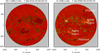 |
Fig. 6 Solar maps corrected for average limb variation of He I 1083.3 nm (left) and Hα (right). Smoothed green contours delineate areas with enhanced emission or absorption with respect to the average line centre intensity. |
Mean  indexes determined from HARPS-N spectra.
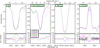 |
Fig. 7 Top panels: mean out-of-transit profiles of Hα, He I 1083.3 nm, Na I D1, and Ca II H (from left to right). The mean profile for each date is drawn with the same colour coding as in Fig. 1. Bottom panels: relative variation from the reference average profile (same colour coding). |
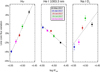 |
Fig. 8 Variation in the central line depth of the mean out-of-transit stellar line profiles as a function of stellar activity as measured bythe |

Correlation coefficients of relative line core variation with the  index (in parentheses the corresponding p-values), and the slopes of the linear fits.
4.4 In-transit He I versus Hα relation
Based on the evidence put forward in the previous section, it appears likely that variability in the planetary helium absorption signal can be due to variations in stellar activity. To put this expectation on more solid ground, we performed a comparative analysis between the He I and the Hα lines to verify the existence of a correlation. We performed optical transmission spectroscopy on each individual primary transit event using the HARPS-N spectra of HD 189733 b in the region around 656.3 nm, following the same method used for the helium nIR triplet (see Sect. 3). By looking at the transmission spectra of all the nights combined together and shown in tomography (see Fig. 9), a strong emission signal emerges at the position of the Hα line, clearly centred in the stellar reference frame. This signal, as it is aligned in the star rest frame, is not due to the planetary atmosphere, but it represents a pseudo-signal caused by the planetary transit over a non-homogeneous stellar disc. By computing the transmission light curve of the Hα line in the planetary rest frame8, we find that the Hα emission signal shown in Fig. 9 comes from two nights out of five (transit 1 and 3), while the other three exhibit constant Hα levels in-transit and out-of-transit (see Fig. 10).
Next, we evaluate night averages of the Hα light curves between contact points t2 and t3. If He I absorption levels are indeed linked to variability in Hα emission, wewould qualitatively expect, for example, stronger absorption levels recorded during transits 1 and 3, in anti-correlation with the stronger Hα emission measured. According to the scenario outlined in Sect. 4.2, this would indicate that the planet was transiting over quiet regions of the stellar surface. As shown by Fig. 11, this is exactly what we see on the third night, meaning that during the transit the planet could have occulted quiescent stellar regions. Moreover, from Fig. 10 we note that the Hα emission signal measured during this transit event seems to last longer than the actual transit. However, we prefer not to draw overly speculative conclusions, as we cannot exclude the possibility that it is simply due to stellar activity by chance aligned with transit.
Instead,a different behaviour is seen during transit 1, as Fig. 5 shows. During transit 1 we do not measureincreased absorption at the position of the helium triplet – in correspondence with an emission in Hα – but a peak in emission in the middle of the transit9. In principle,an emission signal at the position of both lines could be seen if the planet during the transit is passing over a region that is darker than the rest of the stellar disc, both in He I and in Hα. Such an active region could be either a starspot or a filament. To test this possibility, we first checked the RME curve of the first night, to seeif distortions could be present in the RME profile that could be induced by starspot-crossing, but to no avail. To further explore the possible nature of the active region that may have been hidden by the planet during transit 1, we consider the strong Si I 1083.0 nm line. We chose a photospheric rather than a chromospheric line because the latter would also be influenced by the presence of a filament – not only by a starspot like a photospheric line (e.g. the Si I line) – complicating any interpretation regarding the nature of the occulted region. We would expect the Si I 1083.0 nm line to grow weaker in the case of starspot crossing events, while the line strength should be unaffected by the planet hiding a filamentary active region. An analysis of the Si I 1083.0 nm line (not shown) does not highlight any changes in its strength during transit 1. We therefore tentatively conclude that the active region occulted during the transit could be a filament.
We need to stress that in this work we do not take into account the possible planetary contribution to the recorded emission levels for the Hα line. Indeed, our aim is to understand if a qualitative relation could exist between the He I and the Hα lines, and not to perform a fit between the emission and absorption values we find. Nevertheless, the analysis presented here allows us to infer the fact that three out of five transits of HD 189733 b were mostly unaffected by stellar activity, therefore the measured value of planetary He I absorption could be representative of the real one. We make use of this assumption in the next section.
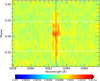 |
Fig. 9 Tomography of the Hα line in the stellar rest frame. A strong signal of stellar origin emerges during transit. Horizontal white lines show the beginning and end of the transit. |
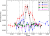 |
Fig. 10 Light curve of Hα. Two nights out of five (transit 1 and 3) show the Hα signal in emission during transit in the stellar reference frame. |
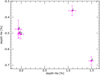 |
Fig. 11 He vs. Hα transit depths. When no in-transit variability of the Hα signal is detected, the He transit depth is constant. |
5 Interpretation of the helium absorption and constraints on the mass loss rate
We select the HD 189733 b transmission spectra obtained for the three transit events that were not significantly affected by stellar activity (transit 2, 4, and 5). The average in-transit absorption depth for the three events is 0.77 ± 0.04% (19σ), a value in excellent agreement (at the ~0.3σ level) with the one calculated considering all the transit events of our dataset (0.75 ± 0.03). We interpret our findings in terms of planetary helium absorption using the EVaporating Exoplanet code (EVE; Bourrier & Lecavelier des Etangs 2013; Bourrier et al. 2016), to take full advantage of the temporal and spectral resolution of the data, and to account for the impact of the stellar surface properties. We use an upgraded version of the EVE code previously applied to observationsof planetary helium lines in Spake et al. (2018), and Allart et al. (2018, 2019) (we refer the reader to these publicationsfor a complete description of the modelling).
The planetary system is simulated in 3D in the stellar rest frame, and the code calculates theoretical spectra comparable to the GIANO-B observations during the transit of the planet. The model star is tiled with the master-out GIANO-B spectrum, scaled in flux according to the continuum limb-darkening in the helium range, and Doppler-shifted according to the orbital motion of the system and the rotational velocity of the star (an obliquity of λ = −0.42 deg, veq = 4.45 km s−1, i* = 92.5°, Cegla et al. 2016). We note that in using the master-out as a proxy for the local stellar lines, we assume that centre-to-limb variations (CLV) can be neglected along the transit chord. This choice is motivated by the absence of spurious residuals induced by CLV in the transmission spectra calculated with the master-out (Fig. 3), and our preference to use the helium spectrum measured directly for HD 189733 rather than theoretical local stellar spectra that we cannot compare with observations. The use of the EVE code allows us to account for the effect of the RME, for limb-darkening, and for the partial occultation of the stellar disc during ingress and egress. Simulations can be compared directly with the observed spectra, with no need to correct them for these effects.
The thermosphere is modelled as a parameterized grid, using density and velocity profiles calculated with a spherically symmetric, steady-state isothermal wind model (Parker 1958). We assume a solar-like hydrogen-helium composition for the thermosphere and set its mean atomic weight to 1.3. In this first interpretation of the GIANO-B spectra we scale the density profile of metastable helium to the density profile of the wind. In future simulations we will calculate more precisely the populations of ground-state and metastable helium (Oklopčić & Hirata 2018). With these settings, the free parameters in the model are the thermosphere temperature, the mass loss of metastable helium, and the extension of the thermosphere. Compared to previous simulations, we account for the rotation of the planet by conferring an angular velocity of 3.28 × 10⁻⁵ s−1 (set by assuming tidal-locking) around the normal direction to the orbital plane to gas in the thermospheric grid.
The theoretical and observed transmission spectra are compared over the spectral range 1082.7–1083.7 nm (in the star rest frame), simultaneously fitting the three nights that show no stellar contamination (transits 2, 4, and 5). We calculate grids of temperature versus mass loss, for an extension of the thermosphere of either 1.2 or 3 RP (i.e. the height of the thermospheric grid is either 0.2 or 2 RP). This choice is motivated by the interpretation of CARMENES observations of HD 189733 b by Salz et al. (2018), which suggest that the helium lines are saturated and could arise from a compact thermosphere well within the Roche lobe at 3 RP. Figure 12 shows the average excess absorption profile (in the planetary rest frame) from the exposures fully in-transit. The best fit (performed by masking the telluric line at 1083.5 nm) yields a reduced χ2 of about 1.18, obtained for an extension of 1.2 RP, a mass loss of metastable helium of ~ 1−2 g s−1 (1σ), and a temperature of 12 000 K.
The data favour hotter thermospheres, but we do not consider temperatures larger than 12 000 K because they are at the upper limit expected for HD 189733 b (see Salz et al. 2016). Figure 13 shows the Δχ2 grid (in confidence level) for the 1.2 RP extension. The best fit for the 3 RP extension is disfavoured with 3σ confidence, in agreement with the Salz et al. (2018) results.
We confirm that the RME has a negligible impact on transmission spectra of HD 189733 b in the region of the helium lines. Spurious signatures induced by the RME are visible in the theoretical spectrum at the location of deep stellar lines,with the W-like shape expected for an aligned system, but their amplitude remains well within the photon noise (Fig. 12). We also note that tidally-locked rotation makes a negligible contribution to the broadening of the helium lines. Our best-fit model has a density of metastable helium of 70 atoms per cm3 at 1.2 RP. This is comparable to the density levels simulated between 1 and 10 RP by Oklopčić & Hirata (2018) for the hot Jupiter HD 209458 b.
As shown by the tomography map in Fig. 3, and the light-curve measurements in Fig. 5, the helium absorption signal seems to start at the t2 contact point and lasts until after the t4 contact point. This suggests that the planet could have an asymmetrical cloud of helium, with a small tail (Rtail < RRoche) that follows the planet, as found for WASP-69b (Nortmann et al. 2018). Moreover, an isotropic, spherical thermosphere model like the one we used, highlights the possible presence of an excess absorption in the blue wing of the lines. We should be cautious about this (because there is no indication of this feature in the CARMENES data), but if confirmed it would suggest (along with the temporal asymmetry we mentioned) the presence of escaping helium atoms blown away from the planet, a scenario that could become the object of future work.
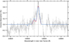 |
Fig. 12 Average excess absorption profile (in the planetary rest frame) from the exposures fully in-transit. The blue profile is the best fitfor 1.2 RP, while the redprofile is the best-fit for 3 RP. Only the three nights that show no stellar contamination (transits 2, 4, and 5) are taken into account. |
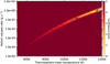 |
Fig. 13 Grid of Δχ2 (in confidence level) for the 1.2 RP thermosphere extension. Black solid lines indicate the 1 and 3σ confidence contours. |
6 Summary and conclusions
We analysed five transits of HD 189733 b acquired with HARPS-N and GIANO-B simultaneously operated in GIARPS observing mode at the TNG. We employed a multi-technique approach (transmission spectroscopy and tomography,transmission spectra equivalent widths, light-curve analysis) to confirm the recent detection of helium in the planet’s extended atmosphere by Salz et al. (2018). We spectrally resolved the He I triplet at 1083.3 nm, and detected an absorption signal on each individual night. The in-transit absorption depth is measured to be 0.75 ± 0.03% (25σ) in the strongest component of the helium triplet. The strength of the average absorption signal is slightly lower than the one (0.88 ± 0.04%) reported by Salz et al. (2018). A possible origin of this difference could be due to the lower resolving power of GIANO-B (R ~ 50 000) compared to that of CARMENES (R ~ 80 400). This could in principle cause extra broadening of the lines and thus a decrease in the lines’ depth. However, we are not in a position to estimate how much this effect amounts to. Investigating in detail the consequences of having two different resolving powers would require a dedicated simulation, which goes beyond the scope of the paper. Moreover in our analysis a night-to-night variability of the helium absorption levels appears rather clear (at the level of 3.3σ and 4σ for night 1 and 3, respectively). We interpret this variability as likely due to the planet transiting inhomogeneities of the active stellar surface. The occultation of quiescent and active regions by the planet during transit can indeed modify the planetary helium absorption signal. This effect is sometimes referred to as the “contrast effect”, and we look for its signatures in other chromospheric lines in addition to the He I triplet, that is, the Hα, the Ca II H and K, and the Na I doublet. If the star presents active regions and the planet transits without hiding them, we expect the weight of active regions in the observed flux to increase, producing a stronger absorption at 1083.3 nm. On the contrary, when the planet passes over active regions, an emission feature is produced in the in-transit transmission spectrum at the position of the He I lines, reducing the helium absorption. On the other hand, the signal perturbations in the Hα (in the Na I doublet and in the Ca II H and K lines) have the opposite behaviour. When the planet hides active regions the total flux in line decreases, while occultation of quiescent regions leads to line flux increase (assuming that the dominant inhomogeneities are plage-like regions).
In order to estimate the role of stellar activity in our He I signal, we first analyse the average stellar spectra outside the transit as a function of stellar activity. From this analysis we find that a nightly variability exists between these out-of-transit spectra and it is consistent with a stellar surface covered by large plage-like active regions.
Encouraged by this empirical evidence, we develop a new approach to evaluate the effects of pseudo-signals induced by stellar activity on the true planetary absorption. The new methodology is based on a comparative analysis of the He I 1083.3 nm (in the infrared) and the Hα (in the visible) lines. The results of this analysis are the following:
-
constant helium absorption signals are recorded in three nights out of five (transit 2, 4, and 5), in correspondence with constant Hα levels in-transit and out-of-transit;
-
one night (transit 3) shows extra absorption in the He I triplet in connection with an emission signal in the Hα line;
-
one transit (transit 1) exhibits a peak in emission during mid-transit both in helium and in Hα.
We interpret the three measurements of constant helium absorption levels (0.77 ± 0.04% on average) as mostly unaffected by stellar activity-induced effects, and therefore representative of the actual absorption by the planetary atmosphere. The anti-correlation observed between the He I 1083.3 nm and Hα signals during transit 3 can be explained as being due to the contrast effect of the presence of active regions (plages) on the stellar disc not covered by the planet during transit. The peaks in emission recorded in transit 1, both at the position of the He I triplet and Hα, can instead be explained as due to the planetary occultation of a stellar filament during transit.
We explain the night-to-night variations in the He I absorption signal as a consequence of the stellar surface geometry (the presence of quiescent and active regions during planetary transit) and not due to stellar variations, such as interaction with stellar wind or flares, or changes in the X-ray and EUV (hereafter XUV) irradiation. Viceversa, variation in the stellar wind and XUV spectrum could instead influence the density of neutral hydrogen resulting in a temporal variation in the in-transit Ly-α signal (Lecavelier Des Etangs et al. 2012; Bourrier et al. 2020). Our feelings are corroborated by the detection of Hα in emission during transit 1 and 3 and not in absorption, as expected by interaction with stellar wind or by variations in the XUV spectrum.
We interpret the HD 189733 b helium absorption observations not significantly affected by stellar contamination (transit 2, 4, and 5) in terms of mass-loss rate using 3D numerical simulations with the EVE code. Our observations are well explained by a compact thermosphere heated to ~12 000 K, extending up to 1.2 planetary radii, well within the Roche lobe (in agreement with previous results by Salz et al. 2018), and losing about ~ 1−2 g s−1 of metastable helium.
In conclusion, active host stars of hot planets such as HD 189733 are promising candidates to search for planetary He I 1083.3 nm absorption from the escaping and extended planetary atmosphere, but absorption in the nIR helium triplet lines due to stellar activity features is a source of serious complications in the interpretation of exoplanet transit observations for active stars. It is therefore of paramount importance to systematically investigate the He I triplet lines alongside diagnostics of stellar activity in other wavelength regimes (e.g. Hα in the optical), using approaches such as the one developed for this work. Only in this way can interpretative degeneracies between actual atmospheric absorption and stellar pseudo-signals be removed and well-determined mass-loss rates be obtained from the measured He I absorption. Hence, the results reported here stress the necessity of simultaneous optical+nIR monitoring when performing high-resolution transmission spectroscopy of the extended and escaping atmospheres of hot planets using facilities such as GIARPS.
Acknowledgements
We want to thank the anonymous referee for the constructive comments which helped to improve the quality of the manuscript. We acknowledge support by INAF/Frontiera through the “Progetti Premiali” funding scheme of the Italian Ministry of Education, University, and Research. G.G. acknowledges the financial support of the 2017 PhD fellowship programme of INAF. P.G. gratefully acknowledges support from the Italian Space Agency (ASI) under contract 2018-24-HH.0. F.B. acknowledges financial support from INAF through the ASI-INAF contract 2015-019-R0. V.B. acknowledges support by the Swiss National Science Foundation (SNSF) in the frame of the National Centre for Competence in Research “PlanetS”. This project has received funding from the European Research Council (ERC) under the European Union’s Horizon 2020 research and innovation programme (project Four Aces, grant agreement no. 724427; project Exo-Atmos grant agreement no. 679633). M.E. acknowledges the support of the DFG priority programme SPP 1992 “Exploring the Diversity of Extrasolar Planets” (HA 3279/12-1).
Appendix A Fringing correction
Fringes in nIR observations often arise from the interference of the incident and internally reflected beams within the thin layers of the detector. In particular, the GIANO-B detector (a Rockwell Scientific HAWAII-2 2048 × 2048 imaging sensor) includes a 0.38 mm sapphire substrate that may generate a near-sinusoidal pattern with a frequency of approximately 7.5 cm−1 in the nIR (seenote 3). There is currently no standard procedure to account for this effect in the standard GIANO-B data processing pipeline. We therefore explore two different methods to remove this pattern from the spectra in the vicinity of the He I 1083.3 nm line, one focused on correcting this effect at the level of the transmission spectra and the other applied to the original spectra.
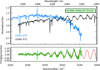 |
Fig. A.1 Fringing correction for transit 3 (upper panels) and transit 1 (lower panels). The mean in-transit transmission spectra in the stellar rest frame for the A-nodding position before the fringing correction, with overplotted Ffrin (in red), areshown in the left panels, while the right panels show the fringing corrected mean spectra. The telluric line residuals are masked (in grey). |
Method #1
We correct our TA (TB), in the stellar rest frame, as follows. For every night, and for each nodding position, we divide the TA (TB) in the stellar rest frame into five groups:
- 1.
before-transit;
- 2.
ingress (between the contact points t1 and t2);
- 3.
in-transit (betwenn the contact points t2 and t3);
- 4.
egress (between the contact points t3 and t4);
- 5.
out-of-transit.
For each of these groups, we build a reference spectrum by averaging on time, and we fit the fringing pattern using the function Ffrin = a0 sin(a1λ + a2) + a3 + a4λ where ai are coefficients and λ is the wavelength. Once the mean fringing pattern fit (Ffrin) has been calculated for each group, we divide each spectrum of each group by the corresponding Ffrin. For transit 1 and 3, Fig. A.1 shows the mean in-transit transmission spectra for the A-nodding position before the fringing correction (left panels) with overplotted Ffrin (in red), and after the fringing removal (right panels).
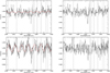 |
Fig. A.2 Example of fringing pattern in the spectrum of a telluric standard. Top panel: spectral orders #70 and #71. Bottom panel: ratio of the two spectral orders after removing the ratio of the blazing functions (green) and its fit (red). |
We wish to underline that the choice to split the transmission spectra into five groups is made a priori to account for any possible time-dependent intra-night fringing variations that might have been introduced during the initial steps of the analysis. In case of a constant fringing pattern throughout the night, the net result is a slight increase in the noise on the fringing correction, with no direct impact on the results of our analysis.
Method #1b
As a consistency check of Method #1, for each night we also calculate the fast Fourier transform (FFT) in the wavelength domain of each transmissionspectrum TA (TB). We then select the two most prominent frequencies of the Fourier spectrum and for them we define the module of the FFT equal to zero. We then perform an inverse transform to bring the data back into the wavelength domain, filtered by the two frequencies previously selected.
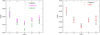 |
Fig. A.3 Comparison between the three fringing correction methods. The EWsAB values for the five nights (x-axis) averaged between the contact point t2 and t3 are plotted. Left panel: results of the three methods (Method #1 in black, Method #1b in magenta, and Method #2 in green). Right panel: comparison between Method #1 and the weighted average of the three methods. |
Method #2
The third method exploits the very different fringing pattern amplitudes in overlapping regions of adjacent spectral orders on the detector. In particular, while the S/N is highest near the He I 1083.3 nm line recorded at spectral order #71, the fringing pattern is practically absent at the wavelengths recorded at order #70 (Fig. A.2, top panel).
If we divide the higher S/N spectrum seen at order #71 by the same spectrum recorded at order #70, both the stellar and the telluric spectrum are removed. Once the ratio of the blaze functions of the two orders is also removed, only the fringing pattern at order #71 is left. Since the amplitude of the pattern varies noticeably in the overlapping range of the two spectral orders (~ 1082−1090 nm), we fit this pattern in wave number as shown in the bottom panel of Fig. A.2using a sine function folded with a Gaussian centred at the peak of the blaze function, k0 (fixed to the value 9267.84 cm−1):
![Mathematical equation: \[ A\:e^{-B\:(k-k_0)^2}\:\sin\left[2\pi(k-k_1)/K\right] + C, \]](/articles/aa/full_html/2020/07/aa37644-20/aa37644-20-eq22.png)
where the free parameters of the fit function are K (the frequency of the pattern), A (the amplitude), B (the scale of attenuation), k1 (the phase), and C (the overall offset).
It is worth noting that the fringing function is remarkably stable across all the datasets we have considered, even though there are some differences among the different transit dates in phase or in amplitude. We also verify that the sine-wave function is a reasonably good approximation in the middle of the overlapping range (1084–1087 nm). The average pattern frequency, in particular, turns out to be 7.66 ± 0.07 cm−1.
Comparison between methods
As the left panel of Fig. A.3 shows, the absorption values obtained at the He I position during the five planetary transits are consistent using these three different techniques. For this reason we are confident with our fringing removal methods. In particular, when performing the data analysis on the transmission spectra during transit, we adopt correction Method #1. Indeed, as shown in the right panel of Fig. A.3, the results from this method are very close to the weighted average of the three methods. Method #2 is adopted for the out-of-transit stellar variability study.
Appendix B In-transit Hα versus Na I versus He I relation
As a consistency check of the analysis presented in Sect. 4.4, we also investigate the behaviour of the stellar Na I D lines. In particular, we focus on the D2 588.9951 nm line as it has a higher line contrast compared to the D1 589.5924 nm line. We use the same light-curve-based approach followed for Hα in Sect. 4.4. A plot of the He I versus Na I D2 transit depths highlights an almost identical behaviour with respect to the He I versus Hα relation, stemming from the direct proportionality between the Hα and Na I D2 signals (see upper and lower panels of Fig. B.1, respectively). This confirms the expectations of similar in-transit behaviour of Hα and Na I lines from the analysis of Sect. 4.3 and agrees with what is expected from modelling efforts by Cauley et al. (2018), thereby reinforcing the reliability of the results presented in Sect. 4.4.
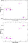 |
Fig. B.1 In-transit Hα vs. Na D2 vs. He I relation. The He vs. Na D2 transit depths (upper panel) follow a similar behaviour to that highlighted by the He I vs. Hα relation (Fig. 11). This is a consequence of the direct proportionality between Na D2 and Hα proxies (lower panel). |
References
- Agol, E., Cowan, N. B., Knutson, H. A., et al. 2010, ApJ, 721, 1861 [NASA ADS] [CrossRef] [Google Scholar]
- Allart, R., Bourrier, V., Lovis, C., et al. 2018, Science, 362, 1384 [NASA ADS] [CrossRef] [Google Scholar]
- Allart, R., Bourrier, V., Lovis, C., et al. 2019, A&A, 623, A58 [NASA ADS] [CrossRef] [EDP Sciences] [Google Scholar]
- Alonso-Floriano, F. J., Snellen, I. A. G., Czesla, S., et al. 2019, A&A, 629, A110 [NASA ADS] [CrossRef] [EDP Sciences] [Google Scholar]
- Andretta, V., & Giampapa, M. S. 1995, ApJ, 439, 405 [NASA ADS] [CrossRef] [Google Scholar]
- Andretta, V., & Jones, H. P. 1997, ApJ, 489, 375 [NASA ADS] [CrossRef] [Google Scholar]
- Andretta, V., Jordan, S. D., Brosius, J. W., et al. 2000, ApJ, 535, 438 [NASA ADS] [CrossRef] [Google Scholar]
- Andretta, V., Mauas, P. J. D., Falchi, A., & Teriaca, L. 2008, ApJ, 681, 650 [NASA ADS] [CrossRef] [Google Scholar]
- Andretta, V., Giampapa, M. S., Covino, E., Reiners, A., & Beeck, B. 2017, ApJ, 839, 97 [Google Scholar]
- Astudillo-Defru, N., & Rojo, P. 2013, A&A, 557, A56 [NASA ADS] [CrossRef] [EDP Sciences] [Google Scholar]
- Barnes, J. R., Haswell, C. A., Staab, D., & Anglada-Escudé, G. 2016, MNRAS, 462, 1012 [Google Scholar]
- Beaugé, C., & Nesvorný, D. 2013, ApJ, 763, 12 [NASA ADS] [CrossRef] [Google Scholar]
- Borsa, F., & Zannoni, A. 2018, A&A, 617, A134 [NASA ADS] [CrossRef] [EDP Sciences] [Google Scholar]
- Bouchy, F., Udry, S., Mayor, M., et al. 2005, A&A, 444, L15 [NASA ADS] [CrossRef] [EDP Sciences] [Google Scholar]
- Bourrier, V., & Lecavelier des Etangs, A. 2013, A&A, 557, A124 [NASA ADS] [CrossRef] [EDP Sciences] [Google Scholar]
- Bourrier, V., Lecavelier des Etangs, A., Dupuy, H., et al. 2013, A&A, 551, A63 [NASA ADS] [CrossRef] [EDP Sciences] [Google Scholar]
- Bourrier, V., Lecavelier des Etangs, A., Ehrenreich, D., Tanaka, Y. A., & Vidotto, A. A. 2016, A&A, 591, A121 [NASA ADS] [CrossRef] [EDP Sciences] [Google Scholar]
- Bourrier, V., Lecavelier des Etangs, A., Ehrenreich, D., et al. 2018, A&A, 620, A147 [NASA ADS] [CrossRef] [EDP Sciences] [Google Scholar]
- Bourrier, V., Wheatley, P. J., Lecavelier des Etangs, A., et al. 2020, MNRAS, 493, 559 [CrossRef] [Google Scholar]
- Brogi, M., Giacobbe, P., Guilluy, G., et al. 2018, A&A, 615, A16 [NASA ADS] [CrossRef] [EDP Sciences] [Google Scholar]
- Carleo, I., Benatti, S., Lanza, A. F., et al. 2018, A&A, 613, A50 [NASA ADS] [CrossRef] [EDP Sciences] [Google Scholar]
- Cauley, P. W., Redfield, S., Jensen, A. G., et al. 2015, ApJ, 810, 13 [NASA ADS] [CrossRef] [Google Scholar]
- Cauley, P. W., Redfield, S., Jensen, A. G., & Barman, T. 2016, AJ, 152, 20 [NASA ADS] [CrossRef] [Google Scholar]
- Cauley, P. W., Redfield, S., & Jensen, A. G. 2017a, AJ, 153, 217 [NASA ADS] [CrossRef] [Google Scholar]
- Cauley, P. W., Redfield, S., & Jensen, A. G. 2017b, AJ, 153, 81 [Google Scholar]
- Cauley, P. W., Kuckein, C., Redfield, S., et al. 2018, AJ, 156, 189 [Google Scholar]
- Cegla, H. M., Lovis, C., Bourrier, V., et al. 2016, A&A, 588, A127 [NASA ADS] [CrossRef] [EDP Sciences] [Google Scholar]
- Charbonneau, D., Brown, T. M., Noyes, R. W., & Gilliland, R. L. 2002, ApJ, 568, 377 [NASA ADS] [CrossRef] [Google Scholar]
- Claudi, R., Benatti, S., Carleo, I., et al. 2017, Eur. Phys. J. Plus, 132, 364 [CrossRef] [Google Scholar]
- Cosentino, R., Lovis, C., Pepe, F., et al. 2012, SPIE Conf. Ser., 8446, 84461V [Google Scholar]
- Drake, G. W. 1971, Phys. Rev. A, 3, 908 [NASA ADS] [CrossRef] [Google Scholar]
- Dupree, A. K., Sasselov, D. D., & Lester, J. B. 1992, ApJ, 387, L85 [NASA ADS] [CrossRef] [Google Scholar]
- Ehrenreich, D., Bourrier, V., Wheatley, P. J., et al. 2015, Nature, 522, 459 [Google Scholar]
- Goldberg, L. 1939, ApJ, 89, 673 [NASA ADS] [CrossRef] [Google Scholar]
- Golding, T. P., Leenaarts, J., & Carlsson, M. 2016, ApJ, 817, 125 [NASA ADS] [CrossRef] [Google Scholar]
- Hirayama, T. 1971, Sol. Phys., 17, 50 [NASA ADS] [CrossRef] [Google Scholar]
- Koen, C., Kilkenny, D., van Wyk, F., & Marang, F. 2010, MNRAS, 403, 1949 [Google Scholar]
- Kohl, S., Salz, M., Czesla, S., & Schmitt, J. H. M. M. 2018, A&A, 619, A96 [CrossRef] [EDP Sciences] [Google Scholar]
- Kulow, J. R., France, K., Linsky, J., & Loyd, R. O. P. 2014, ApJ, 786, 132 [NASA ADS] [CrossRef] [Google Scholar]
- Lavie, B., Ehrenreich, D., Bourrier, V., et al. 2017, A&A, 605, L7 [NASA ADS] [CrossRef] [EDP Sciences] [Google Scholar]
- Lecavelier Des Etangs, A. 2007, A&A, 461, 1185 [NASA ADS] [CrossRef] [EDP Sciences] [Google Scholar]
- Lecavelier Des Etangs, A., Ehrenreich, D., Vidal-Madjar, A., et al. 2010, A&A, 514, A72 [NASA ADS] [CrossRef] [EDP Sciences] [Google Scholar]
- Lecavelier des Etangs, A., Bourrier, V., Wheatley, P. J., et al. 2012, A&A, 543, L4 [NASA ADS] [CrossRef] [EDP Sciences] [Google Scholar]
- Leighly, K. M., Dietrich, M., & Barber, S. 2011, ApJ, 728, 94 [NASA ADS] [CrossRef] [Google Scholar]
- Lundkvist, M. S., Kjeldsen, H., Albrecht, S., et al. 2016, Nat. Commun., 7, 11201 [Google Scholar]
- MacPherson, K. P., & Jordan, C. 1999, MNRAS, 308, 510 [NASA ADS] [CrossRef] [Google Scholar]
- Mansfield, M., Bean, J. L., Oklopčić, A., et al. 2018, ApJ, 868, L34 [NASA ADS] [CrossRef] [Google Scholar]
- Mazeh, T., Holczer, T., & Faigler, S. 2016, A&A, 589, A75 [NASA ADS] [CrossRef] [EDP Sciences] [Google Scholar]
- Moutou, C., Coustenis, A., Schneider, J., Queloz, D., & Mayor, M. 2003, A&A, 405, 341 [NASA ADS] [CrossRef] [EDP Sciences] [Google Scholar]
- Nortmann, L., Pallé, E., Salz, M., et al. 2018, Science, 362, 1388 [NASA ADS] [CrossRef] [EDP Sciences] [Google Scholar]
- Oklopčić, A. 2019, ApJ, 881, 133 [NASA ADS] [CrossRef] [Google Scholar]
- Oklopčić, A., & Hirata, C. M. 2018, ApJ, 855, L11 [NASA ADS] [CrossRef] [Google Scholar]
- Oliva, E., Origlia, L., Baffa, C., et al. 2006, SPIE Conf. Ser., 6269, 626919 [Google Scholar]
- Owen, J. E., & Lai, D. 2018, MNRAS, 479, 5012 [NASA ADS] [CrossRef] [Google Scholar]
- Parker, E. N. 1958, ApJ, 128, 664 [Google Scholar]
- Rainer, M., Harutyunyan, A., Carleo, I., et al. 2018, SPIE Conf. Ser., 10702, 1070266 [Google Scholar]
- Salz, M., Czesla, S., Schneider, P. C., & Schmitt, J. H. M. M. 2016, A&A, 586, A75 [NASA ADS] [CrossRef] [EDP Sciences] [Google Scholar]
- Salz, M., Czesla, S., Schneider, P. C., et al. 2018, A&A, 620, A97 [NASA ADS] [CrossRef] [EDP Sciences] [Google Scholar]
- Seager, S., & Sasselov, D. D. 2000, ApJ, 537, 916 [NASA ADS] [CrossRef] [Google Scholar]
- Snellen, I. A. G., Albrecht, S., de Mooij, E. J. W., & Le Poole, R. S. 2008, A&A, 487, 357 [NASA ADS] [CrossRef] [EDP Sciences] [Google Scholar]
- Spake, J. J., Sing, D. K., Evans, T. M., et al. 2018, Nature, 557, 68 [NASA ADS] [CrossRef] [EDP Sciences] [Google Scholar]
- Triaud, A. H. M. J., Queloz, D., Bouchy, F., et al. 2009, A&A, 506, 377 [NASA ADS] [CrossRef] [EDP Sciences] [Google Scholar]
- Vidal-Madjar, A., Lecavelier des Etangs, A., Désert, J.-M., et al. 2003, Nature, 422, 143 [NASA ADS] [CrossRef] [PubMed] [Google Scholar]
- Vidal-Madjar, A., Arnold, L., Ehrenreich, D., et al. 2010, A&A, 523, A57 [NASA ADS] [CrossRef] [EDP Sciences] [Google Scholar]
- Weidmann, W. A., Gamen, R., van Hoof, P. A. M., et al. 2013, A&A, 552, A74 [NASA ADS] [CrossRef] [EDP Sciences] [Google Scholar]
- Wyttenbach, A., Ehrenreich, D., Lovis, C., Udry, S., & Pepe, F. 2015, A&A, 577, A62 [NASA ADS] [CrossRef] [EDP Sciences] [Google Scholar]
- Yan, F., & Henning, T. 2018, Nat. Astron., 2, 714 [NASA ADS] [CrossRef] [Google Scholar]
- Zarro, D. M., & Zirin, H. 1986, ApJ, 304, 365 [NASA ADS] [CrossRef] [Google Scholar]
- Zirin, H. 1975, ApJ, 199, L63 [NASA ADS] [CrossRef] [Google Scholar]
In this paper we use vacuum wavelengths for GIANO-B and air wavelengths for HARPS-N. This is due to the type of reference system selected as default by the reduction software used.
Given the negligible impact of the Rossiter-McLaughlin effect (RME) during transit on the analysis and interpretation of the planetary helium absorption signal (see Sect. 5 and Salz et al. 2018), we do not correct for it.
We adopt here the following definition for the equivalent width measured in the stellar spectra: Wλ = ∫ (1 − (F(λ)∕Fcont) dλ where F(λ) is the flux line profile and Fcont is the flux in the adjacent stellar continuum; the equivalent width thus defined is a positive quantity for absorption lines.
We choose the planetary rest frame to be coherent with the helium analysis, but since we average over a velocity range of ±20 km s−1, ± 0.44 Å, centred on the Hα line, the results do not change if we derive the light curves in the stellar rest frame.
As a consistency check, a very similar behaviour is seen by using the Sodium doublet as a proxy instead of Hα. See Appendix B.
All Tables
Average peak absorption in the strongest He I component in each individual night.
Averaged He I transit depths in each individual night between contact points t2 and t3 in the transmission light curves.
Correlation coefficients of relative line core variation with the index (in parentheses the corresponding p-values), and the slopes of the linear fits.
All Figures
|
Fig. 1 Airmass during the GIARPS observations. The colour and symbol coding presented here will be adopted consistently throughout the work. The contact points t1 and t4 are marked with vertical dashed lines. |
| In the text | |
|
Fig. 2 Telluric absorptions spectrum built for the highest S/N night considering only the GIANO-B A-spectra. As a comparison,the telluric spectrum generated via the ESO SKy Model Calculator is shown in blue with an offset of −0.3. The two spectra are consistent. In our telluric spectrum the fringing pattern affecting GIANO-B spectra is also visible. |
| In the text | |
|
Fig. 3 Transmission spectra shown in tomography in the planetary (left) and stellar (right) rest frame, as a function of the wavelength and the orbital phase (transmission spectra are binned both in wavelength and in phase). An excess absorption (in blue) is present during the transit, the three helium triplet lines are indicated with vertical black lines. The contact point t1, t2, t3 and t4 are marked with horizontal white lines. |
| In the text | |
|
Fig. 4 Mean TAB of the five observed nights in the planetary rest frame. We detect an average absorption signal of 0.75 ± 0.03% (25σ) in the strongest component of the helium triplet. A Gaussian fit is shown as the red line. Vertical dashed lines indicate the three helium triplet lines. |
| In the text | |
|
Fig. 5 Left panel: transmission light curve of the He I lines in the planetary rest frame from the five transits. Contact points t1, t2, t3, and t4 are marked with vertical dashed lines. Right panel: transmission light curve, binned in phase, obtained for the five nights combined. Contact points t1, t2, t3, and t4 are marked with dashed lines. The continuum behaviour is indicated by the horizontal dashed line. |
| In the text | |
|
Fig. 6 Solar maps corrected for average limb variation of He I 1083.3 nm (left) and Hα (right). Smoothed green contours delineate areas with enhanced emission or absorption with respect to the average line centre intensity. |
| In the text | |
|
Fig. 7 Top panels: mean out-of-transit profiles of Hα, He I 1083.3 nm, Na I D1, and Ca II H (from left to right). The mean profile for each date is drawn with the same colour coding as in Fig. 1. Bottom panels: relative variation from the reference average profile (same colour coding). |
| In the text | |
|
Fig. 8 Variation in the central line depth of the mean out-of-transit stellar line profiles as a function of stellar activity as measured bythe |
| In the text | |
|
Fig. 9 Tomography of the Hα line in the stellar rest frame. A strong signal of stellar origin emerges during transit. Horizontal white lines show the beginning and end of the transit. |
| In the text | |
|
Fig. 10 Light curve of Hα. Two nights out of five (transit 1 and 3) show the Hα signal in emission during transit in the stellar reference frame. |
| In the text | |
|
Fig. 11 He vs. Hα transit depths. When no in-transit variability of the Hα signal is detected, the He transit depth is constant. |
| In the text | |
|
Fig. 12 Average excess absorption profile (in the planetary rest frame) from the exposures fully in-transit. The blue profile is the best fitfor 1.2 RP, while the redprofile is the best-fit for 3 RP. Only the three nights that show no stellar contamination (transits 2, 4, and 5) are taken into account. |
| In the text | |
|
Fig. 13 Grid of Δχ2 (in confidence level) for the 1.2 RP thermosphere extension. Black solid lines indicate the 1 and 3σ confidence contours. |
| In the text | |
|
Fig. A.1 Fringing correction for transit 3 (upper panels) and transit 1 (lower panels). The mean in-transit transmission spectra in the stellar rest frame for the A-nodding position before the fringing correction, with overplotted Ffrin (in red), areshown in the left panels, while the right panels show the fringing corrected mean spectra. The telluric line residuals are masked (in grey). |
| In the text | |
|
Fig. A.2 Example of fringing pattern in the spectrum of a telluric standard. Top panel: spectral orders #70 and #71. Bottom panel: ratio of the two spectral orders after removing the ratio of the blazing functions (green) and its fit (red). |
| In the text | |
|
Fig. A.3 Comparison between the three fringing correction methods. The EWsAB values for the five nights (x-axis) averaged between the contact point t2 and t3 are plotted. Left panel: results of the three methods (Method #1 in black, Method #1b in magenta, and Method #2 in green). Right panel: comparison between Method #1 and the weighted average of the three methods. |
| In the text | |
|
Fig. B.1 In-transit Hα vs. Na D2 vs. He I relation. The He vs. Na D2 transit depths (upper panel) follow a similar behaviour to that highlighted by the He I vs. Hα relation (Fig. 11). This is a consequence of the direct proportionality between Na D2 and Hα proxies (lower panel). |
| In the text | |
Current usage metrics show cumulative count of Article Views (full-text article views including HTML views, PDF and ePub downloads, according to the available data) and Abstracts Views on Vision4Press platform.
Data correspond to usage on the plateform after 2015. The current usage metrics is available 48-96 hours after online publication and is updated daily on week days.
Initial download of the metrics may take a while.