| Issue |
A&A
Volume 639, July 2020
|
|
|---|---|---|
| Article Number | A64 | |
| Number of page(s) | 10 | |
| Section | Galactic structure, stellar clusters and populations | |
| DOI | https://doi.org/10.1051/0004-6361/202037591 | |
| Published online | 07 July 2020 | |
Extended stellar systems in the solar neighborhood
IV. Meingast 1: the most massive stellar stream in the solar neighborhood⋆,⋆⋆
1
Data Science at University of Vienna, Währinger Straße 29, 1090 Vienna, Austria
e-mail: This email address is being protected from spambots. You need JavaScript enabled to view it.
2
University of Vienna, Department of Astrophysics, Türkenschanzstrasse 17, 1180 Wien, Austria
3
Radcliffe Institute for Advanced Study, Harvard University, 10 Garden Street, Cambridge, MA 02138, USA
4
University of Vienna, Faculty of Computer Science, Währinger Straße 29/S6, 1090 Vienna, Austria
5
University of Vienna, ISOR/VCOR, Oskar-Morgenstern-Platz 1, 1090 Vienna, Austria
Received:
27
January
2020
Accepted:
11
April
2020
Abstract
Context. Nearby stellar streams carry unique information on the dynamical evolution and disruption of stellar systems in the Galaxy, the mass distribution in the disk, and they provide unique targets for planet formation and evolution studies. Recently, Meingast 1, a 120° stellar stream with a length of at least 400 pc, was dicovered.
Aims. We aim to revisit the Meingast 1 stream to search for new members within its currently known 400 pc extent, using Gaia DR2 data and an innovative machine learning approach.
Methods. We used a bagging classifier of one-class support vector machines with Gaia DR2 data to perform a 5D search (positions and proper motions) for new stream members. The ensemble was created by randomly sampling 2.4 million hyper-parameter realizations admitting classifiers that fulfill a set of prior assumptions. We used the variable prediction frequency resulting from the multitude of classifiers to estimate a stream membership criterion, which we used to select high-fidelity sources. We used the HR diagram and the Cartesian velocity distribution as test and validation tools.
Results. We find about 2000 stream members with high fidelity, or about an order of magnitude more than previously known, unveiling the stream’s population across the entire stellar mass spectrum, from B stars to M stars, including white dwarfs. We find that, apart from being slightly more metal poor, the HRD of the stream is indistinguishable from that of the Pleiades cluster. For the mass range at which we are mostly complete, ∼0.2 M⊙ < M < ∼4 M⊙, we find a normal IMF, allowing us to estimate the total mass of stream to be about 2000 M⊙, making this relatively young stream by far the most massive one known. In addition, we identify several white dwarfs as potential stream members.
Conclusions. The nearby Meingast 1 stream, due to its richness, age, and distance, is a new fundamental laboratory for star and planet formation and evolution studies for the poorly studied and gravitationally unbound star formation mode. We also demonstrate that one-class support vector machines can be effectively used to unveil the full stellar populations of nearby stellar systems with Gaia data.
Key words: methods: statistical / open clusters and associations: individual: Meingast 1 / stars: luminosity function, mass function / stars: massive / stars: low-mass / white dwarfs
The full source catalog described in Table G.1 is only available at the CDS via anonymous ftp to cdsarc.u-strasbg.fr (130.79.128.5) or via http://cdsarc.u-strasbg.fr/viz-bin/cat/J/A+A/639/A64
In our original discovery paper, we did not name the stream. The authors of the first follow-up paper (Curtis et al. 2019) contacted us regarding a name for the structure but did not agree with our proposed name and decided on their own to name the system the Pisces-Eridanus stream. Their chosen name, however, not only does not capture the true size of the stream (the stream stretches across at least 10 constellations and likely extends beyond these), it is ambiguous as it can lead to confusion with the Pisces moving group (Binks et al. 2018). In general, given the number of new streams being found by Gaia and the finite number of constellations, it seems appropriate to move away from using constellations to name streams (e.g., Ibata et al. 2019). An unambiguous remedy to this particular situation is to name the stream after the original discoverer, which we do in this paper, naming the structure Meingast 1.
© ESO 2020
1. Introduction
Coherently moving groups of stars in the Milky Way are unique laboratories where we can coherently study a large variety of astrophysical processes. For instance, the similar birth conditions in nearby moving groups have provided much insight into individual stellar properties (e.g., Torres et al. 2008; Gagné et al. 2014; Riedel et al. 2017, and references therein). Moreover, while older stellar systems experience mass loss due to the gravitational interaction with the Galaxy’s gravitational potential (e.g., Meingast & Alves 2019; Röser et al. 2019), young co-moving groups can give us important clues on the governing star formation processes in the Milky Way.
Recently, Meingast et al. (2019), the second installment in this series (hereinafter referred to as Paper II), discovered a 120° stellar stream that is currently traversing the immediate solar neighborhood at a distance of only ∼100 pc. For this paper, the authors determined the age of the system to be 1 Gyr. Their assumption was mostly based on the presence of a single star in their selection, namely the subgiant 42 Ceti. Shortly after the stream’s discovery, Curtis et al. (2019) determined stellar rotation periods of stream members to be very similar to stars in the Pleiades. Their application of gyrochronolgy thus sets the age of the stream at close to 120 Myr, implying that the star 42 Ceti is likely an unfortunate interloper.
The search criteria in Paper II were based on the 3D space velocities in a cylindrical coordinate frame derived from astrometric measurements provided with the second Gaia data release (Gaia DR2; Gaia Collaboration 2016, 2018c). While space velocities provide a robust estimate on membership, evaluating 3D motions of stars requires radial velocity measurements. This requirement substantially limits the identification of members to a small subset of Gaia DR2, specifically to stars with G ≲ 13 mag, which in the case of Meingast 1 translate to stellar masses between ∼0.5 and 1.5 M⊙.
The goal of this paper is to unveil the stellar population of the Meingast 1 stream, from B stars down to mid-M stars, or the completeness limit of the Gaia DR2 data. To this end, we applied state-of-the-art machine learning tools, where we used the previously identified members as a training set. The structure of this paper is as follows: in Sect. 2, we present the data used for the analysis. Section 3 summarizes the method used to select potential stream member sources from the Gaia DR2 data set. Finally, in Sect. 4, we present a final high-fidelity source catalog on which we determine the age and mass of the Meingast 1 stream1.
2. Data
For the analysis, we used the 5D position (α, δ, ϖ) and velocity (μα, μδ) information, provided by Gaia DR2. Following the data selection in Paper II, we preferred distance estimates provided by Bailer-Jones et al. (2018). The distance limit of the stellar sample is kept at ≤300 pc in accordance with Paper II. This is motivated by the choice of our classifier, which predicts member stars within the limits of the previously determined extent of the stream. Furthermore, the subsequently described method works independently from quality criteria. Therefore, quality filters are only applied for visualisation purposes. This selection results in a data set of 18 692 951 total stars.
For Paper II, the sources were extracted in a 6D parameter space spanned by three spatial (X, Y, Z) and three velocity dimensions (vr, vϕ, vz). Specifically, the velocities were represented in a galactocentric cylindrical coordinate system to better represent the bulk motion stars. Consequently, the source identification in Paper II depended on radial velocity measurements, which are scarce in Gaia DR2. Within the search region of 300 pc, about 95% of all sources in the catalog were, therefore, not taken into account in Paper II due to missing radial velocity data.
3. Member selection
As mentioned above, the bulk of Gaia DR2 catalog sources were not used in the original member identification of the stream in Paper II. Omitting the radial velocity component yields a much more complete source list, but at the same time limits any analysis to projected tangential velocities given by the proper motion measurements. While members of spatially confined star clusters can be identified reliably in proper motion space, the recently discovered stream encompasses at least 120° on sky. This large extent introduces significant projection effects in tangential velocities, posing a nontrivial problem for member identification in 5D.
3.1. Supervised member selection
To avoid the difficult task of clustering in the 5D position and proper motion space, we pursued a supervised approach based on one-class support vector machines (OCSVM; Schölkopf et al. 2001). Instead of finding a decision boundary between distinct groups in the training sample like a typical SVM (Cortes & Vapnik 1995), an OCSVM constructs a decision surface that attains a maximum separation between the training samples and the origin. Consequently, the algorithm infers the properties of the input samples by enclosing the support of its joint distribution with a hyper surface during the training process. Depending on the position of unseen data points2 to this surface, a trained predictor acts as a binary function which groups new example points as either resembling the previously seen training data or not. We aim to estimate the extent of the stellar stream by using the OCSVM algorithm and the already classified sources from Paper II as a training set. Subsequently, we predict the membership of unseen stars to the stream within a 300 pc sphere around the Sun (see Sect. 2). In order to find a model that is capable of providing a physically meaningful characterization of the stellar stream in the 5D feature space, the corresponding hyper-parameters of the OCSVM classifier have to be set sensibly.
3.2. Parameter tuning
We made use of the libsvm (Chang & Lin 2011) OCSVM implementation, which features two main hyper-parameters for the RBF-kernel3, γ and ν. The parameter γ defines a region of influence of the support vectors selected by the model. The variable ν controls the fraction of possible outliers as well as the fraction of support vectors. Thus, γ and ν are crucial hyper-parameters that define the shape of the enveloping hull.
Additionally, these parameters, and subsequently the classifier shape, depend on the input variable range. Since the parameter γ describes a support vector region of influence, different feature ranges lead to a varying model flexibility within each input variable. To mitigate an asymmetric feature weighting, a common approach is to standardize each input variable to a common variance by dividing each feature by its standard deviation. However, as we are dealing with a combined feature space of position and proper motion information a certain weighting towards one of the two feature spaces might be beneficial to properly characterize the joint probability of stream members. Consequently, after scaling the features to unit variance, we added an additional hyper-parameter: cx/cv. This parameter describes the scaling fraction between positional and proper motion features. When cx/cv = 1 the variance in both feature spaces is the same. In practice, we set cv = 1 and vary cx within a certain range.
As we chose a classifier via a set of hyper-parameters, we have to be aware of existing contamination in the training set (estimated to amount to a few percent in Paper II). Additional selection biases caused by the original clustering and parameter choice that influence the final obtained stream selection should be considered. Therefore, only crude estimates about the true joint distribution of the sources in 5D are possible. Nevertheless, we have information about the resulting classifier shape, which limits the space of possible solutions. Firstly, based on the number of missing radial velocity measurements, we estimate that the total number of member stars should roughly increase twenty-fold. Secondly, due to a lack of a better description we estimate that the true extent is comparable to the original selection in Paper II, which found that the stream is roughly prolate spheroidal with a length of about 400 pc and an equatorial diameter of about 50 pc.
A trained classifier has to be able to capture these prior assumptions. Therefore, we used the above mentioned characteristics to eliminate predictions that seem unfit to describe the stellar stream in 5D. Since we cannot infer the true joint distribution from the available stream members, and our prior assumptions entail some allowable margin of variation, the model parameters cannot be tuned to optimal values. Instead, we aggregated the predictions of multiple models that conform to our prior assumptions into an ensemble of OCSVMs. This procedure is referred to as bootstrap aggregating, also known as bagging (Breiman 1996). A benefit of using multiple aggregated classifiers, in comparison to one single model, is an improvement in prediction stability. Due to its variance-reducing ability, bagging has been successfully applied, especially to noise-prone classifiers, whose predictions vary significantly with small variations in the training data. In Grandvalet (2004), the author suggests that bagging systematically reduces the influence of outlier samples in the training data. Furthermore, by bundling together multiple models, a notion of stability for each star is obtained as different regions of the 5D training space have varying prediction frequencies. Ideally, the ensemble of classifiers has a higher prediction frequency towards the center region of the stellar stream (in 5D) where sources are less likely to be randomly selected field stars. Bagging, therefore, automatically creates a hierarchy from more robust to less robust stream members, which reduces prediction variance compared to a single classifier.
A schematic illustration of a small ensemble classifier is shown in Fig. 1. The black scatter points represent the training set, whereas the colored shapes depict the bounding surfaces of individual OCSVM classifiers trained with different sets of hyper-parameters. The unification of multiple classifiers results in an ensemble classifier where overlapping bounding regions result in different levels of prediction frequency.
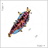 |
Fig. 1. Schematic figure illustrating the effect of different hyper-parameters on the classifier shape in the Galactic X–Y plane. Black points represent the training set, whereas the colored shapes depict the bounding surfaces of individual OCSVM classifiers trained with a different set of hyper-parameters. The unification of multiple classifiers results in an ensemble classifier where overlapping bounding regions result in different levels of stability. |
The final bagging predictor is obtained in a two step process: Firstly, the actual training phase and, secondly, the validation phase, which rejects models that do not represent our expectations well. In the learning phase (see Appendix A for more details) the model is trained using ten-fold cross validation on a random set of hyper-parameters (γi, νi, (cx/cv)i). Before deploying the classifier on the full data set, we filtered out models below a mean accuracy score of 0.5, or a standard deviation above 0.15 across the hold-out sets. Models passing this filter criterion enter the validation phase, which assess the classifiers capability of capturing our prior assumptions about the distribution and quantity of predicted sources. We require the model to comply with the following criteria. Firstly, the number of predicted stream members Ns must not exceed a physically sensible range, which is limited to Ns ∈ [500, 5000]. Secondly, the extent of the predicted stream members in position and proper motion space must be similar to the original ones. Thirdly, the cylindrical velocity distribution of the stream members must not deviate too much from the training sample distribution. For a full description on the implementation of these three validation criteria, see Appendix B.
Since we cannot formulate an exact objective function to be minimized, we did not converge to a single, optimal hyper-parameter selection. Instead, the models were assessed as either plausible candidates, which capture out prior assumptions about the distribution of the predicted sources, or not. Therefore, for small ensemble classifiers with only a few models, the prediction depends on the sampling strategy in hyper-parameter space. To reduce the dependency on the search strategy, we iterate through 2.4 million random realizations of (γi, νi, (cx/cv)i) within their respective range in order to converge to a stable solution. Altogether, the final classifier ensemble consists of a total of 8515 classifiers, which have passed the validation steps. Figure C.1 shows the distribution of accepted models with respect to the hyper-parameters ν, γ, and cx/cv. The software used to train the ensemble classifier is publicly available4.
3.3. Limitations and caveats
Any supervised model based on OCSVMs is limited by the provided training data, because the shape of the decision surface is determined by the input training set. As suggested in Paper II, the stream’s extent might potentially be much larger due to sensitivity limitations. The method used in this paper is not able to infer the stream membership of stars outside the constructed decision boundary. Finding externally located stream members would require, for example, a transition to unsupervised methods, which are not limited by a fixed training set.
Additionally, the constructed decision boundary depends heavily on the outermost points in the training sample as they are more likely to act as support vectors for the decision surface. As the density of points decreases towards these outer regions (in 5D), the decision boundary depends on random fluctuations of these border points present in the training set. Furthermore, we suspect the fraction of contaminants in stream member stars per unit volume increase towards border regions. Thus, outliers in the border region have an increasing chance of being a support vector defining the shape of the decision surface. These effects, however, are somewhat mitigated by the choice of bagging multiple predictors, which helps to reduce unstable decision surfaces.
While omitting the radial velocity component opens up the possibility to search for more stream members, we lose, at the same time, an additional discriminative dimension. By neglecting the radial velocity distribution of the input data, the implemented classification scheme impacts the contaminant fraction of our final source list. This leads to an increasing recall at the cost of reduced precision.
4. Results and discussion
Using no pre-filter selection the classifier ensemble predicts a total of 4243 stream members. This source list does not, however, contain all members from the original training set. Approximately 10% of the training data are not captured by the ensemble classifier. This reduction can be attributed to the model validation phase, where we prioritized more conservative models in an attempt to prevent overfitting. To increase this retrieval rate, we would need to omit the bootstrapping step combined with the subsequent majority voting (see Appendix A) and use the entire sample to train individual classifiers. Also, to be sensitive to more remote points, we would need to include more flexible models in the classifier ensemble. However, these tools and choices have been installed to prevent serious overfitting on the training data and to dampen the influence of outlier samples in the training data. Since an important goal is to find a robust model that minimizes the contamination fraction of the inferred points, we tolerate a slightly reduced retrieval fraction of the original training set points.
To visualize our results, we implemented a series of quality selections described in Appendix D, hereinafter referred to as filter Q1. For a direct comparison to the original training sample, we implemented the filter criteria as in Paper II (excluding the criterion on radial velocities), hereinafter referred to as filter Q2. The quality filters Q1 and Q2 reduce the total number of classified member stars to 2567 and 2913, respectively. This selection contains, however, many sources that are predicted by only a marginal fraction of the 8515 classifiers in the bagging ensemble. Each individual classifier is associated with an individual set of classified stream members. Thus, considering all 8515 classifiers, each source can be assigned a prediction frequency. We define this prediction frequency, hereinafter referred to as stability, as the fraction of classifiers in the bagging ensemble that include a certain star in their prediction set. Figure 2 shows the 5D distribution of the training sample (top row) and the stream members classified by our trained OCSVM (quality filter Q1), where the color indicates the stability of each source for our new classification. We observe that, on average, stability values tend to increase towards the central parts of the stream. Additionally, we find that when inspecting the new source set in the color-absolute magnitude diagram (see Fig. 5), sources with lower stability numbers correlate with a larger scatter, while sources with higher stability values are more compactly distributed around an idealized isochronal curve. Therefore, stability can be used as a measure to filter out potential contaminant sources.
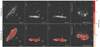 |
Fig. 2. Positional and proper motion projections of the training and prediction set are displayed in the first and second rows, respectively. Using a quality pre-selection (see Appendix D), we find a total of 2567 member stars (bottom row), compared to 256 in the training set (top row). The color information highlights the stability of a given star, which tends to grow towards the central regions of the stream. |
Since the training process includes a validation step, even stars with low stability values can be regarded as potential stream members. Hence, stability constitutes not a probability estimate, but rather a quality feature for which we aim to find a suitable criterion to clean our prediction sample. To determine the reliability of the predicted stellar sample, we estimated the level of contamination at various stability filters.
We measured the contamination via the velocity dispersion in 3D, parametrized via vr, vϕ, and vz. However, due to contributions of random contaminants, the standard error of the prediction set is largely dominated by outliers, regardless of the stability filter criterion. Hence, we describe the variability of the velocity distribution with the median absolute deviation (MAD), which is a robust estimate of statistical dispersion. For reference, the training data distribution measures an MAD in the 3D velocities of 2.1 km s−1.
Figure 3 displays the influence of a variable stability filter criterion on the 3D velocity distribution. By moving in the plot from left to right, we gradually added less “stable” sources to the predicted data set. We identified two distinct sections in this curve that are dominated by different slopes. Firstly, the section with stabilities from 100% decreasing to 4% is comprised of a roughly constant growing scatter around the expected 3D Cartesian velocity. Secondly, adding sources with a stability below ∼4% results in a rapid growth of the MAD. This sudden increase is most likely caused by adding a significant number of contaminating field stars. Here, we assumed that these contaminating field stars are more likely associated with the outer borders of the stream in the 5D parameter space, which is also where the trained classifier ensemble is less confident about the stream membership of stars. This decrease in stability values of predicted sources towards the outer regions of the stream is also well visible in Fig. 2.
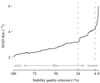 |
Fig. 3. Median absolute deviation of sources from expected 3D velocity as a function of the stability quality filter. The x-axis is reversed displaying very strict filter criteria on the leftmost side and lenient filter criteria toward the right side. A trend is visible where the amount of scatter over the stability filter is split into two parts, where each is characterized by a different slope. Suitable quality filters are realized by stability > 4% and, more conservatively, stability > 24%. |
In addition to the sudden increase at 4%, we identify another characteristic property of the MAD distribution in Fig. 3. Starting at about 40%, we observe an extended flat distribution up to 24%. In this range, the amount of scatter remains nearly constant. This filter criterion (stability ≥24%) yields a very stable subsample to the more lenient stability > 4% criterion.
The filter behavior can be observed in more detail in Fig. 4, where the successive cleaning of the prediction set is displayed in each individual velocity component. The solid lines in the figure represent a kernel density estimation of the marginal distributions for various color-coded stability filter criteria. Specifically, we sampled the distributions at constant intervals in stability with a step size of 5%. The hue change from red to shades of blue indicates the transition from a contamination-dominated to a more robust filter regime. In the marginal distributions, the disproportionately large reduction in the amount of scatter around mean velocities by applying the stability > 4% filter criterion becomes apparent. For subsequent filter criteria, the contamination outside the training sample distribution (black line) is reduced at a nearly constant rate, particularly in the vr and vϕ observables. Moreover, we identify a kinematic substructure in the panel displaying vz velocities. Sources identified with this substructure have systematically larger vertical velocities by about 5 km s−1 compared to the bulk motion of the stream. These sources are only clearly separable in vz and do not show any obvious correlation in other velocities or can be segregated in spatial coordinates. We note here that this substructure accounts for the high MAD of the predicted sources and is removed only for very conservative stability filter criteria above 90%.
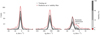 |
Fig. 4. Kernel density estimation of marginal 3D velocity distributions for various stability filter criteria. The individual lines are color-coded by the filter criteria and range from red (stability < 4%) to dark blue, which represents the strictest filter criterion. The distributions are sampled at constant intervals in stability with a step size of 5%. The hue change from red to shades of blue indicates the transition from the contamination dominated to the more robust filter regime. In addition, we note a kinematic substructure in the z-velocity distribution which is indistinguishable from other sources in all features except vz. |
Following the above outlined characteristics in the velocity distributions, we therefore implemented an additional criterion of stability > 4% or stability > 24% for a more conservative approach. Depending on the quality filter selection, the stability > 4% filter criterion reduces the number of predicted stream members to 1869 or 2110 for Q1 and Q2, respectively.
In order to quantify the contamination fraction in our source catalog, we considered the fraction of outliers in the marginal 3D velocity distributions. To do this, we defined, for each velocity component, a region of inliers as the 3σ around the training sample mean. This definition constitutes a very conservative estimate, as the velocity distribution of the training data is by design very narrow. Furthermore, the kinematic substructure in the vz component naturally leads to very large contamination fractions. For this reason, we only considered the radial and azimuthal velocity components when estimating the contamination for various stability filter criteria. Figure 6 shows the outlier fraction within each velocity component. Based on our assumptions, we obtain a contamination estimate of roughly 25% and 20% for the stability criteria > 4% and > 24%, respectively. However, we note again that this is a very conservative estimate that assumes an intrinsic velocity dispersion of only around 1 km s−1. By increasing the estimated velocity dispersion to 2 km s−1 the contamination drops to roughly 10−15%, which we suspect to be a more realistic estimate.
Since the ensemble classifier is trained on positional and proper motion data, we can apply it to any survey that provides these measurements. In an effort to increase the source list, especially toward brighter stars, we applied our ensemble classifier to the HIPPARCOS (van Leeuwen 2007) source catalog, see Appendix F for more details. In total, we find 21 new potential stream members in the HIPPARCOS catalog, 10 of which we consider to be robust. We added the 10 predicted HIPPARCOS sources to the HRD plot in Fig. 5. Among the prediction set, we find α Aquarii, the brightest star in the Aquarius constellation. Using the radial velocity information from Soubiran et al. (2008), we find a galactocentric velocity of v = (− 3.15, 229.19, −8.73) km s−1, which is well within the 3σ region of the training set. However, a comparison of parallax measurements between Gaia and HIPPARCOS reveals a large systematic discrepancy of a factor of approximately two, which makes α Aquarii a low-fidelity stream member.
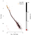 |
Fig. 5. Distribution of predicted sources in color-absolute magnitude diagram. The shades of gray encode the stability information of each source. The hue change in the color map at 4% denotes the transition from robust stream members in gray tones to less reliable sources in red. Additionally, we show 10 new potential stream members, identified by applying the same classifier to the HIPPARCOS catalog. |
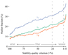 |
Fig. 6. Outlier fraction in individual velocity components for a variable stability filter criterion. Due to a newly identified kinematic substructure in vz, we estimate the contamination only in the radial and azimuthal velocity components (see Sect. 4). Based on this premise, the contamination is estimated to be roughly 25% and 20% for the stability criteria > 4% and > 24%, respectively. |
Using gyrochronology, Curtis et al. (2019) concluded that the stream has an age comparable to the Pleiades. This contrasted with the isochronal age derived in Meingast et al. (2019), which was hinging on a single star, 42 Ceti, a subgiant. With the new and larger member list, we can now attempt to make a more precise estimate regarding the stream’s age.
We compared the stream to a selection of the Pleiades members (Gaia Collaboration 2018a). By introducing a slight color offset of (GBP–GRP + 0.03) to the stream, we find that the source distributions in the HRD of the Meingast 1 stream and the Pleiades match almost perfectly, as seen in Fig. 7, implying a similar age between the two stellar systems. The small color shift could imply either the presence of dust extinction towards the Pleiades, or a lower metallicity of the stream, or both. The Pleiades are known to be affected by small amounts of extinction. Additionally, we find a slight metallicity difference between the stream and the Pleiades measured by LAMOST Liu et al. (2015), which is illustrated Fig. E.1. The plot shows a discrepancy between the mean metallicity fraction of the two stellar populations, where sources in Meingast 1 appear to be slightly more metal poor than the ones in the Pleiades, which could help to explain the reddening in color space.
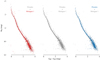 |
Fig. 7. Comparison between predicted stream members and the Pleiades member selection. The three panels show the same two data sets plotted on top of each other and highlighted by different colors. In the left plot, the predicted stream members are highlighted in red, while the Pleiades are kept in gray. The center plot displays both stellar associations in gray. The right plot displays the Pleiades member selection in blue on top of the predicted stellar stream in gray. We chose the stability cut to match the number of sources in the Pleiades sample in order to generate a fair comparison. The CMD distributions of the Pleiades and the predicted stream matches almost perfectly. |
The three panels in Fig. 7 show the source distributions in the HRD of both, the Meingast 1 stream and the Pleiades, plotted on top of each other and highlighted by different colors. In the left plot, sources in the Meingast 1 stream are highlighted in red, while the Pleiades members selection are kept in gray. The center plot displays both stellar populations, which are shown in gray. The right plot displays the Pleiades in blue on top of Meingast 1 in gray. In order to make a fair comparison, we define the stability filter in such a way that the number of sources of the stream is equal to that of the Pleiades. This results in the following filter criterion: stability > 45.9. The particular similarity of the two distributions suggests an approximately identical age. The Gaia collaboration (Gaia Collaboration 2018b) estimates the age and metallicity fraction of the Pleiades to be 110 My and Z = 0.017, respectively. Therefore, our age estimate is within the expected error range, consistent with Curtis et al. (2019).
We estimated the total mass of the selected sources in accordance with Paper II by using PARSEC isochrones. Using an age estimate of 110 My and a metallicity fraction of Z = 0.016 results in the mass distribution shown in Fig. 8. The plot depicts the mass distribution of the training samples (dark blue) versus the predicted samples (light blue). The dotted gray lines indicate IMFs (Kroupa 2001) for clusters masses of 1000 M⊙, 2000 M⊙, and 3000 M⊙. A comparison to the model IMFs suggests an approximate mass of 2000 M⊙, as suggested in Paper II. To our knowledge, this makes the Meingast 1 stream the most massive stellar stream in the solar neighborhood.
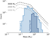 |
Fig. 8. Mass function for Meingast 1 stream sources (light blue) and the training examples (dark blue). The dotted lines indicate model IMFs within a cluster mass range of 1000−3000 M⊙. |
Finally, we can speculate on the origin of the Meingast 1 stream. In Paper II, we put forward the possible cluster versus association scenarios for the origin of this extended structure, but opted not to favor one over the other, even though we found evidence for the existence of at least four overdensities in the structure. This ambiguity resulted mainly from the older age derived in Paper II, which made it not obvious to favor one of the two scenarios without a proper simulation. The much younger age determined in Curtis et al. (2019), that we confirm in this work, allowed these authors to favor the association scenario (because ∼100 Myr is too short for cluster dissolution). The best and most obvious example is the Pleiades cluster, which is a relatively compact cluster with essentially the same age as Meingast 1. The velocity substructure we found in this paper (see Fig. 4) now allows us to make a stronger case favoring the association scenario as the likely initial configuration of Meingast 1. Unlike compact clusters, stellar associations such as Sco-Cen are known to have velocity substructures of a few to several km s−1 (e.g., Wright & Mamajek (2018), Goldman et al. (2018)). A more meaningful look into the origin of Meingast 1, which would require n-body simulations and the effects of the Galactic potential, will enable us to clarify the origin of this mesmerizing structure.
5. Summary and conclusion
We revisited the stream discovered in Meingast et al. (2019) to search for new members using Gaia DR2 data and a machine-learning approach. Using the original source selection as training data, we deployed a bagging classifier of one-class support vector machines to the full Gaia DR2 data, searching for new stream members in position and tangential velocity space. The ensemble classifier is created in a hyper-parameter search combined with a model selection that rejects models that do not meet a set of preconditions. The resulting set of classifiers creates a variable prediction frequency for possible stream member stars, which we used as a criterion to select high-fidelity sources. Subsequently, we validated the newly found sources in the HR diagram and the Cartesian velocity distribution.
In total, we find about 2000 stream high-fidelity member stars, increasing the source population approximately tenfold. As the newly predicted stream members are no longer limited by radial velocity measurements, the new selection substantially extends the main sequence to unveil the stream’s population across the entire stellar mass spectrum, from B stars to M stars, including white dwarfs. In a comparison in the color-absolute magnitude diagram, we find that, apart from being slightly more metal poor, the stream is indistinguishable from that of the Pleiades cluster, suggesting a similar age. In the mass range at which we are mostly complete, ∼0.2 < M⊙ < ∼4 M⊙, we identify a normal IMF. This comparison allows us to estimate the total mass of the stream to approximately 2000 M⊙, making it by far the most massive stream we know. Additionally, we find several white dwarfs as members of the stream. We speculate with more confidence, given the velocity substructure found in this work, that Meingast 1 is the likely outcome of a stellar association, but call for a full, state-of-the-art simulation to be done to characterize the origin of this mesmerizing structure.
We acknowledge the simultaneous publication by Röser & Schilbach (2020), who have also studied member stars of the Meingast 1 stream.
Stars in the data set are represented as points in a 5D space with three position axes and two proper motion axes constituting the so-called feature space. Thus, in a machine learning context, we refer to stars in the data set as points in a feature space.
We conclude from extensive hyper-parameter searches that the RBF kernel always outperformed the alternative options. Hence we omit the description of other kernel types in this section.
Nearby refers to sources in the vicinity of the stellar stream in the5D feature space.
Acknowledgments
We thank the anonymous referee for his insightful comments that helped to improve this study. This work has made use of data from the European Space Agency (ESA) mission Gaia (https://www.cosmos.esa.int/gaia), processed by the Gaia Data Processing and Analysis Consortium (DPAC, https://www.cosmos.esa.int/web/gaia/dpac/consortium). Funding for the DPAC has been provided by national institutions, in particular the institutions participating in the Gaia Multilateral Agreement. This research made use of Astropy, a community-developed core Python package for Astronomy (Astropy Collaboration 2018). We also acknowledge the various Python packages that were used in the data analysis of this work, including NumPy (van der Walt et al. 2011), SciPy (Virtanen et al. 2019), scikit-learn (Pedregosa et al. 2011), Pandas (McKinney et al. 2010), and Matplotlib (Hunter 2007). This research has made use of the SIMBAD database operated at CDS, Strasbourg, France (Wenger et al. 2000)
References
- Astropy Collaboration (Price-Whelan, A. M., et al.) 2018, AJ, 156, 123 [Google Scholar]
- Bailer-Jones, C. A. L., Rybizki, J., Fouesneau, M., Mantelet, G., & Andrae, R. 2018, AJ, 156, 58 [NASA ADS] [CrossRef] [Google Scholar]
- Binks, A. S., Jeffries, R. D., & Ward, J. L. 2018, MNRAS, 473, 2465 [NASA ADS] [CrossRef] [Google Scholar]
- Breiman, L. 1996, Mach. Learn., 24, 123 [Google Scholar]
- Bressan, A., Marigo, P., Girardi, L., et al. 2012, MNRAS, 427, 127 [NASA ADS] [CrossRef] [Google Scholar]
- Chang, C.-C., & Lin, C.-J. 2011, ACM Trans. Intell. Syst. Technol., 2, 1 [NASA ADS] [CrossRef] [MathSciNet] [Google Scholar]
- Cortes, C., & Vapnik, V. 1995, Mach. Learn., 20, 273 [Google Scholar]
- Curtis, J. L., Agüeros, M. A., Mamajek, E. E., Wright, J. T., & Cummings, J. D. 2019, ApJ, 158, 77 [Google Scholar]
- Gagné, J., Lafrenière, D., Doyon, R., Malo, L., & Artigau, É. 2014, ApJ, 783, 121 [NASA ADS] [CrossRef] [Google Scholar]
- Gaia Collaboration (Prusti, T., et al.) 2016, A&A, 595, A1 [NASA ADS] [CrossRef] [EDP Sciences] [Google Scholar]
- Gaia Collaboration 2018a, VizieR Online Data Catalog: J/A+A/616/A10 [Google Scholar]
- Gaia Collaboration (Babusiaux, C., et al.) 2018b, A&A, 616, A10 [NASA ADS] [CrossRef] [EDP Sciences] [Google Scholar]
- Gaia Collaboration (Brown, A. G. A., et al.) 2018c, A&A, 616, A1 [NASA ADS] [CrossRef] [EDP Sciences] [Google Scholar]
- Goldman, B., Röser, S., Schilbach, E., Moór, A. C., & Henning, T. 2018, ApJ, 868, 32 [NASA ADS] [CrossRef] [Google Scholar]
- Grandvalet, Y. 2004, Mach. Learn., 55, 251 [CrossRef] [Google Scholar]
- Hunter, J. D. 2007, Comput. Sci. Eng., 9, 90 [NASA ADS] [CrossRef] [Google Scholar]
- Ibata, R. A., Malhan, K., & Martin, N. F. 2019, ApJ, 872, 152 [NASA ADS] [CrossRef] [Google Scholar]
- Kroupa, P. 2001, MNRAS, 322, 231 [NASA ADS] [CrossRef] [Google Scholar]
- Lindegren, L. 2018, Re-normalising the astrometric chi-square in Gaia DR2, Technical Report GAIA-C3-TN-LU-LL-124-01 [Google Scholar]
- Lindegren, L., Hernández, J., Bombrun, A., et al. 2018, A&A, 616, A2 [NASA ADS] [CrossRef] [EDP Sciences] [Google Scholar]
- Liu, X.-W., Zhao, G., & Hou, J.-L. 2015, Res. Astron. Astrophys., 15, 1089 [CrossRef] [Google Scholar]
- McKinney, W. 2010, in Data structures for statistical computing in python, eds. S. van der Walt, & J. Millman, Proc. 9th Python Sci. Conf, 51 [Google Scholar]
- Meingast, S., & Alves, J. 2019, A&A, 621, L3 [NASA ADS] [CrossRef] [EDP Sciences] [Google Scholar]
- Meingast, S., Alves, J., & Fürnkranz, V. 2019, A&A, 622, L13 (Paper II) [NASA ADS] [CrossRef] [EDP Sciences] [Google Scholar]
- Pedregosa, F., Varoquaux, G., Gramfort, A., et al. 2011, J. Mach. Learn. Res., 12, 2825 [Google Scholar]
- Riedel, A. R., Blunt, S. C., Lambrides, E. L., et al. 2017, AJ, 153, 95 [NASA ADS] [CrossRef] [Google Scholar]
- Röser, S., & Schilbach, E. 2020, A&A, 638, A9 [CrossRef] [EDP Sciences] [Google Scholar]
- Röser, S., Schilbach, E., & Goldman, B. 2019, A&A, 621, L2 [NASA ADS] [CrossRef] [EDP Sciences] [Google Scholar]
- Schölkopf, B., Platt, J. C., Shawe-Taylor, J. C., Smola, A. J., & Williamson, R. C. 2001, Neural Comput., 13, 1443 [CrossRef] [Google Scholar]
- Soubiran, C., Bienaymé, O., Mishenina, T. V., & Kovtyukh, V. V. 2008, A&A, 480, 91 [NASA ADS] [CrossRef] [EDP Sciences] [Google Scholar]
- Torres, C. A. O., Quast, G. R., Melo, C. H. F., & Sterzik, M. F. 2008, Young Nearby Loose Associations, 5, 757 [Google Scholar]
- van der Walt, S., Colbert, S. C., & Varoquaux, G. 2011, Comput. Sci. Eng., 13, 22 [Google Scholar]
- van Leeuwen, F. 2007, A&A, 474, 653 [NASA ADS] [CrossRef] [EDP Sciences] [Google Scholar]
- Virtanen, P., Gommers, R., Oliphant, T. E., et al. 2019, SciPy 1.0-Fundamental Algorithms for Scientific Computing in Python [Google Scholar]
- Wenger, M., Ochsenbein, F., Egret, D., et al. 2000, A&AS, 143, 9 [NASA ADS] [CrossRef] [EDP Sciences] [Google Scholar]
- Wright, N. J., & Mamajek, E. E. 2018, MNRAS, 476, 381 [NASA ADS] [CrossRef] [Google Scholar]
Appendix A: Training process
The training of each individual predictor in the full model ensemble is summarized in the following two steps.
Firstly, we select a random pair of hyper-parameters (γi, νi, (cx/cv)i) and train a model with tenfold cross validation (CV). Due to a contamination of field stars of a few percent in Paper II, we encourage stricter and more compact descriptions of the stream (in 5D), ignoring potential outliers in the training sample. In a first selection step, we filter models with a low average accuracy across the holdout sets of < 0.5 or a standard deviation of above 0.15. The standard deviation filter helps to obtain fairly conclusive predictors for different subsamples on a fixed set of hyper-parameters.
Secondly, models that pass the CV step are deployed on the full data set (see Sect. 2). In an effort to minimize contamination of nearby5 field stars and thus boost robustness of the prediction, we train the model on 10 bootstrap samples, with a sample size of 80% of the training data size. The union of all 10 predictions is then considered the final model. Before we add the newly trained model (with the hyper-parameter set (γi, νi, (cx/cv)i) into the final bagging classifier, we validate its performance against our prior beliefs about the approximate model structure described in Sect. 3.2
Appendix B: Validation process
After training a classifier, we validate its ability to capture important physical aspects about the estimated size and shape of the stellar stream. We require the classifier to capture at least the following criteria:
1. The number of predicted stream members Ns must not exceed a physically sensible range, which is limited to Ns ∈ [500, 5000].
2. The extent of the predicted stream members in position and proper motion space must be similar to the original ones.
3. The cylindrical velocity distribution of the stream members must not deviate too much from the training sample distribution.
The similarity condition (2.) is achieved by requiring the dispersion of the predicted to the original stream members in position and proper motion space to be approximately equal. We approximate the extent, or dispersion of the stream in both spaces by a single number, namely the mean distance  of its member stars to the centroid of the full stream. For a point in position space r = (x, y, z) and its corresponding centroid rc,
  is
is
 (B.1)
(B.1)
where N is the number of stars belonging to the cluster. Respectively, in proper motion space with a point v = (μα, μδ) and centroid vc,  is:
is:
 (B.2)
(B.2)
We use these two structure parameters  and
and  to determine the extent of the stream in position and proper motion space, respectively. Our aim is to find models whose predicted points retain a similar dispersion to the original ones. To avoid overfitting, we compare the dispersion of the prediction set to the training set which acts as an upper limit:
 (B.3)
(B.3)
Lastly, we control the centroid position of the predicted stream members to avoid systematic shifts. The predicted and original stream centroid must be reasonably close to each other with respect to the average dispersion of training points.
 (B.4)
(B.4)
 (B.5)
(B.5)
The third condition is implemented by examining the contamination of predicted samples compared to the training sample. To get a rough estimate of the contamination, we compare the galactocentric velocity distribution, meaning v = (vr, vϕ, vz), of the predicted sources to the training sample. Instead of comparing the velocity dispersion of both samples, we characterize the level of contamination by considering the fraction of outlier sources. This way, we try to mitigate the influence of large outliers, which increase the dispersion drastically for such a low number of sources. In order to characterize outlier sources, we consider the training examples. Assuming that almost all sources lie within the ±3σ range around the mean, we consider the ratio of sources lying outside of the 3σ range compared to the total amount of sources. A classifier is rejected if on average, across the individual velocity components, more than 25% of sources are considered outliers. The aim of this criterion is to remove models that extend into a region of feature space where the radial velocity distribution does not match our assumption of a co-moving structure.
Appendix C: Parameter tuning results
The hyper-parameter search in combination with a classifier selection and validation step (see Sect. 3.2) yields a set of approvedparameter triples (νi, γi, (cx/cv)i) that make up the final OCSVM bagging predictor. The distribution of accepted triples is displayed in Fig. C.1. The color information illustrates the accepted model faction within a certain hyper-parameter bin range. A model is accepted if it passes the quality criteria presented in Sect. 3.2. The model ensemble consists of 8515 individual predictors.
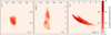 |
Fig. C.1. Hyper-parameter search in parameters ν, γ, and cx/cv yielding the one-class support vector machine bagging predictors. The color information illustrates the accepted model faction within a certain hyper-parameter bin range. A classifier is accepted if it passes the quality criteria presented in Sect. 3.2. The model ensemble consists of 8515 individual predictors. |
Appendix D: Quality criteria
In general, the source identification method we present in this paper is independent of any quality criteria. However, in order to show the distribution of stars in the color magnitude diagram, we apply the following error criteria on data quality. Following the description in Lindegren et al. (2018) the five-parameter solution depends on the number of visibility periods used for a certain source. A visibility period is defined as a group of observations separated from other groups by a gap of at least four days. Since a five-parameter solution is accepted only for visibility_periods_used > 6, we implement said criterion.
A recommended astrometric quality parameter is the re-normalised unit weight error (RUWE) described by Lindegren (2018). It is based on a re-calibration of the unit weight error described in Lindegren et al. (2018). We follow the advice in the technical note (Lindegren 2018) and use the criterion RUWE < 1.4 to select astrometrically reliable sources. Furthermore, we implement additional astrometric quality measures, astrometric_sigma_5D_max < 0.5 and ϖ/σϖ > 10, which reduce the number erroneous measurements.
Finally, we adopt the following photometric quality criteria, phot_bp_mean_flux_over_error > 10 and phot_rp_mean_flux_over_error > 10.
Appendix E: Metal content
Figure E.1 shows a comparison of the metallicity fraction Z between a Pleiades member selection (Gaia Collaboration 2018a) and the stream members. A cross-match of the Pleiades and stream source selections to the LAMOST DR5 Liu et al. (2015) catalog results in 383, and 83 matches, respectively. The conversion from chemical abundance ratios [Fe/H] to the metallicity fraction Z has been made in accordance with the PARSEC (Bressan et al. 2012) solar value of Z = 0.015. Subsequently, we filter out the most untrustworthy sources by requiring that the error of the measured chemical abundance ratios [Fe/H] is below 0.05 and [Fe/H] > − 1. Additionally, we only select sources above an effective temperature of 5000 K. These criteria yield 197 and 44 matched sources for the Pleiades and the Meingast 1 stream, respectively. The metal content distributions of the Pleiades and stream members show a large scatter, but the positions of their respective mean indicate that the Meingast 1 stream members appear to be slightly more metal poor compared to the Pleiades member stars.
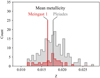 |
Fig. E.1. Comparison of metallicity fraction of Pleiades and Meingast 1 memeber stars. The vertical lines indicate the mean metal content of both populations. We find that the members of the Meingast 1 associtation are slightly more metal poor than the Pleiades. |
Appendix F: HIPPARCOS source selection
Compared to the training samples from the Gaia DR2 catalog, the HIPPARCOS sources have larger associated standard errors of measured quantities. Considering the higher uncertainty in the HIPPARCOS catalog variables, we adopt a more conservative stability filter criterion of stability > 50%. Despite a rather high stability cut, a large standard error increases the chance of contaminant stars falling into the selection. Therefore, we adopt a second quality filter where we sample each data point from marginal normal distributions centered on the provided mean value with a standard deviation of the provided standard error of each observable. We then draw 100 samples per source from these marginal distributions and count how often these re-sampled sources are again predicted to be a stream members with stability > 50%. Eventually, this quality criterion yields 11 additional sources with a re-sampling fraction of over 50%.
Appendix G: Table content
The content of the published source catalog is summarized in Table G.1.
Contents of the source catalog, which are available online via CDS.
All Tables
All Figures
|
Fig. 1. Schematic figure illustrating the effect of different hyper-parameters on the classifier shape in the Galactic X–Y plane. Black points represent the training set, whereas the colored shapes depict the bounding surfaces of individual OCSVM classifiers trained with a different set of hyper-parameters. The unification of multiple classifiers results in an ensemble classifier where overlapping bounding regions result in different levels of stability. |
| In the text | |
|
Fig. 2. Positional and proper motion projections of the training and prediction set are displayed in the first and second rows, respectively. Using a quality pre-selection (see Appendix D), we find a total of 2567 member stars (bottom row), compared to 256 in the training set (top row). The color information highlights the stability of a given star, which tends to grow towards the central regions of the stream. |
| In the text | |
|
Fig. 3. Median absolute deviation of sources from expected 3D velocity as a function of the stability quality filter. The x-axis is reversed displaying very strict filter criteria on the leftmost side and lenient filter criteria toward the right side. A trend is visible where the amount of scatter over the stability filter is split into two parts, where each is characterized by a different slope. Suitable quality filters are realized by stability > 4% and, more conservatively, stability > 24%. |
| In the text | |
|
Fig. 4. Kernel density estimation of marginal 3D velocity distributions for various stability filter criteria. The individual lines are color-coded by the filter criteria and range from red (stability < 4%) to dark blue, which represents the strictest filter criterion. The distributions are sampled at constant intervals in stability with a step size of 5%. The hue change from red to shades of blue indicates the transition from the contamination dominated to the more robust filter regime. In addition, we note a kinematic substructure in the z-velocity distribution which is indistinguishable from other sources in all features except vz. |
| In the text | |
|
Fig. 5. Distribution of predicted sources in color-absolute magnitude diagram. The shades of gray encode the stability information of each source. The hue change in the color map at 4% denotes the transition from robust stream members in gray tones to less reliable sources in red. Additionally, we show 10 new potential stream members, identified by applying the same classifier to the HIPPARCOS catalog. |
| In the text | |
|
Fig. 6. Outlier fraction in individual velocity components for a variable stability filter criterion. Due to a newly identified kinematic substructure in vz, we estimate the contamination only in the radial and azimuthal velocity components (see Sect. 4). Based on this premise, the contamination is estimated to be roughly 25% and 20% for the stability criteria > 4% and > 24%, respectively. |
| In the text | |
|
Fig. 7. Comparison between predicted stream members and the Pleiades member selection. The three panels show the same two data sets plotted on top of each other and highlighted by different colors. In the left plot, the predicted stream members are highlighted in red, while the Pleiades are kept in gray. The center plot displays both stellar associations in gray. The right plot displays the Pleiades member selection in blue on top of the predicted stellar stream in gray. We chose the stability cut to match the number of sources in the Pleiades sample in order to generate a fair comparison. The CMD distributions of the Pleiades and the predicted stream matches almost perfectly. |
| In the text | |
|
Fig. 8. Mass function for Meingast 1 stream sources (light blue) and the training examples (dark blue). The dotted lines indicate model IMFs within a cluster mass range of 1000−3000 M⊙. |
| In the text | |
|
Fig. C.1. Hyper-parameter search in parameters ν, γ, and cx/cv yielding the one-class support vector machine bagging predictors. The color information illustrates the accepted model faction within a certain hyper-parameter bin range. A classifier is accepted if it passes the quality criteria presented in Sect. 3.2. The model ensemble consists of 8515 individual predictors. |
| In the text | |
|
Fig. E.1. Comparison of metallicity fraction of Pleiades and Meingast 1 memeber stars. The vertical lines indicate the mean metal content of both populations. We find that the members of the Meingast 1 associtation are slightly more metal poor than the Pleiades. |
| In the text | |
Current usage metrics show cumulative count of Article Views (full-text article views including HTML views, PDF and ePub downloads, according to the available data) and Abstracts Views on Vision4Press platform.
Data correspond to usage on the plateform after 2015. The current usage metrics is available 48-96 hours after online publication and is updated daily on week days.
Initial download of the metrics may take a while.