| Issue |
A&A
Volume 639, July 2020
|
|
|---|---|---|
| Article Number | A18 | |
| Number of page(s) | 16 | |
| Section | Stellar structure and evolution | |
| DOI | https://doi.org/10.1051/0004-6361/201937305 | |
| Published online | 02 July 2020 | |
The nature of the companion in the Wolf-Rayet system EZ Canis Majoris
1
Instituto de Ciencias Físicas, Universidad Nacional Autónoma de México, Ave. Universidad S/N, Cuernavaca, 62210 Morelos, México
e-mail: gloria@icf.unam.mx, gloria@astro.unam.mx
2
Physikalisch-Meteorologisches Observatorium Davos and World Radiation Center, Dorfstrasse 33, 7260 Davos Dorf, Switzerland
e-mail: werner.schmutz@pmodwrc.ch
Received:
12
December
2019
Accepted:
29
April
2020
Context. EZ Canis Majoris is a classical Wolf-Rayet star whose binary nature has been debated for decades. It was recently modeled as an eccentric binary with a periodic brightening at periastron of the emission originating in a shock heated zone near the companion.
Aims. The focus of this paper is to further test the binary model and to constrain the nature of the unseen close companion by searching for emission arising in the shock-heated region.
Methods. We analyze over 400 high resolution International Ultraviolet Explorer spectra obtained between 1983 and 1995 and XMM-Newton observations obtained in 2010. The light curve and radial velocity (RV) variations were fit with the eccentric binary model and the orbital elements were constrained.
Results. We find RV variations in the primary emission lines with a semi-amplitude K1 ∼ 30 km s−1 in 1992 and 1995, and a second set of emissions with an anti-phase RV curve with K2 ∼ 150 km s−1. The simultaneous model fit to the RVs and the light curve yields the orbital elements for each epoch. Adopting a Wolf-Rayet mass M1 ∼ 20 M⊙ leads to M2 ∼ 3−5 M⊙, which implies that the companion could be a late B-type star. The eccentric (e = 0.1) binary model also explains the hard X-ray light curve obtained by XMM-Newton and the fit to these data indicates that the duration of maximum is shorter than the typical exposure times.
Conclusions: The anti-phase RV variations of two emission components and the simultaneous fit to the RVs and the light curve are concrete evidence in favor of the binary nature of EZ Canis Majoris. The assumption that the emission from the shock-heated region closely traces the orbit of the companion is less certain, although it is feasible because the companion is significantly heated by the WR radiation field and impacted by the WR wind.
Key words: binaries: close / binaries: spectroscopic / stars: Wolf-Rayet / stars: winds / outflows / X-rays: binaries / ultraviolet: stars
© ESO 2020
1. Introduction
EZ Canis Majoris (EZ CMa, HD 50896, WR6; van der Hucht 2001) is one of the brightest Wolf-Rayet (WR) stars that is accessible from the Northern Hemisphere. It is a classical WR star, possessing a strong and fast wind in which the abundances of He and N are enriched compared to typical main sequence stars in the Galaxy. The high ionization stage of the emission lines that are present in its spectrum point to a high effective temperature, and lead to its classification as a nitrogen-rich, high ionization WR star, WN4. It is one of over 400 WR stars known in our Galaxy1, objects that are considered to be in a short-lived, late evolutionary state, soon to end their life in a supernova event.
Gaia observations indicate that EZ CMa is located at a distance of d ∼ 2.27 kpc and they confirm its large distance from the galactic plane, z ∼ 380 pc (Rate & Crowther 2020). It is surrounded by an X-ray emitting HII region, with abundances indicative of material ejected by the WR wind (Toalá et al. 2012).
For close to 80 years, the possible binary nature of EZ CMa has been a topic of debate, with early observations suggesting periodicities in the range of 1–13 d (Wilson 1948; Ross 1961; Kuhi 1967; Lindgren et al. 1975; Schmidt 1974). A stable period ∼3.7 d was finally shown to exist (Firmani et al. 1978, 1980), and subsequently confirmed by numerous investigations as summarized in Robert et al. (1992), Duijsens et al. (1996), and Georgiev et al. (1999). The unseen companion was proposed to be a low-mass object, possibly a neutron star, as evolutionary scenarios call for the existence of such systems (van den Heuvel et al. 1976). However, it was soon found that, although the 3.7 d period is always present in the data, the phase-dependent variability is not coherent over timescales longer than a couple of weeks (Drissen et al. 1989; Robert et al. 1992). This conclusion was contested by Georgiev et al. (1999), who found that the variations in the N V λλ4603, 4621 P Cygni absorptions appeared to show coherent variability over a 15 year timeframe. Thus, the debate has continued. Recently, Schmutz & Koenigsberger (2019, henceforth SK19) successfully fit a binary model to the high-precision photometric observations obtained by the BRITE-Constellation satellite system (Moffat et al. 1995b). The basic conclusion of Schmutz & Koenigsberger (2019) is that the lack of coherence over long timescales can be attributed to a rapidly precessing eccentric orbit.
In the model presented by SK19, the wind of the WR star collides upon a nondegenerate, low-mass companion forming a hot and bright shock region which gives rise to excess emission. The presence of such a companion was previously suggested by Skinner et al. (2002) based on the X-ray spectral energy distribution and luminosity. The intensity of the excess emission depends on the orbital separation, being brightest at periastron which is when the companion enters deeper into the WR wind. Thus, times at which overall brightness increases are associated with periastron passage. At times of conjunction, a portion of the bright shock-heated region is occulted by the star that lies closer to us. This leads to eclipses, as observed in the BRITE data, and gives times of conjunction. Our model was inspired by the results obtained for the WR+O binary system γ2 Velorum where both the emission from the colliding wind and its eclipses were identified (Lamberts et al. 2017; Richardson et al. 2017). In the case of EZ CMa, however, instead of two colliding winds we assume only one wind which produces the shock near the companion’s surface.
In this paper we apply the same analysis as in SK19 to X-ray and ultraviolet (UV) data of HD 50896 with the aim of further testing the model and constraining the nature of the unseen companion. In Sect. 2 we describe the observational material and the measurements. In Sect. 3 we summarize the method of analysis which is then applied to the X-ray light curve obtained by XMM-Newton. In Sect. 4 we analyze four sets of International Ultraviolet Explorer (IUE) observations to constrain the radial velocity curves of the 3.7 d orbit. The results are discussed in Sect. 5 and the conclusions summarized in Sect. 6. Supporting material is provided in Appendix A.
2. Observational material
The observational material has been in its majority reported previously and is summarized in Table 1. It consists of observations obtained with XMM-Newton in 2010 and with the IUE in 1983, 1988, 1992, and 1995.
Summary of data sets.
The XMM-Newton data were obtained with EPIC and are fully described in Oskinova et al. (2012). The IUE spectra were retrieved from the INES data base2. The Short Wavelength Prime (SWP) spectra cover the wavelength range of ∼1180–1970 Å and were obtained with the high resolution grating with exposure times in the range of 200–240 s. These spectra are described in Willis et al. (1989), St. -Louis et al. (1993, 1995) and Massa et al. (1995). All IUE spectra are flux-calibrated with the INES IUE data processing pipeline. No correction for reddening has been applied.
The dominant observational effect caused by the collision of the WR wind with the companion is the production of line emission (Lamberts et al. 2017; Richardson et al. 2017). Thus, for the analysis of IUE spectra, we chose spectral bands centered on some of the principal emission and absorption features and computed the total flux contained within them as follows:
where λ1, λ2 are the initial and final wavelengths of the band, Fλ is the flux given in ergs cm−2 s−1 Å−1, and dλ is the wavelength increment which for the SWP data is 0.05 Å. The advantage of using Fλ (as opposed to Fλ − Fc, with Fc a continuum level) lies in that it avoids the challenges inherent to determining a continuum level, which in UV spectra is very uncertain due to the density of emission lines.
For the velocity measurements, we obtained the flux-weighted average wavelength, defined as:
with λ1 < λ < λ2. The choice of this method is based on the fact that the time-varying asymmetry of emission lines leads to different velocity values depending on the method that is used (gaussian/voigt/lorentz fit; or bisector of flux average or bisector of the extension of the line wings), and on whether the entire line or only a portion is measured. Hence, it provides a uniform and automated method to measure the large number of IUE spectra. The disadvantage of the method is that when the variable component is weak and superposed on a stronger, less variable emission, the RVs of the weaker feature are diluted. Thus, in a second pass, the variable superposed features were measured interactively with Gaussian fits.
The wavelength bands that were tested for flux variability are listed in Table 2. They were chosen to cover portions of emission and absorption lines. In addition, we chose a spectral band (Fc1840) which is relatively free of emission lines in order to characterize the continuum variability.
UV wavelength bands.
3. The binary model and the X-ray light curve
3.1. Description of the model
The binary star model that was introduced in SK19 is based on the following premises: (1) the WR star wind collides with its unseen companion and the resulting shock region emits radiation in wavelengths ranging from X-rays to radio; (2) the intensity of the emitted radiation is proportional to the wind density, (which decreases with orbital separation) so in the eccentric orbit, a larger flux is emitted at periastron than at apastron; (3) the companion is a low mass object that does not possess a stellar wind; (4) since the shock emission is constrained to a relatively small volume and this volume lies very close to the secondary star, portions of the enhanced emitting region can be eclipsed not only by the WR star but also by the low-mass companion. The eclipses are treated as Gaussian-shaped dips in the light curve, with the duration and the strength of the eclipse as free parameters.
In more detail, we compute the intensity variations as a function of time of a localized region that orbits the WR star under the assumption that the variation is caused by an increase or decrease of the energy density. Neglecting the variation in wind velocity, this reduces to variations in the wind particle density, ne. The process responsible for the localized nature of the emission is the collision of the WR wind on the unseen companion. Because of the eccentric orbit, the value of ne varies over the orbital cycle and therefore so does the emission intensity arising in the shock, which is assumed to follow a d−2 relation, with d the orbital separation3.
This computation yields a light curve having a maximum at the time of periastron. However, the orbital precession causes the times of periastron to advance (or recede) compared to a constant anomalistic period, PA. Our binary model performs a fit to the observations by iterating over PA and  (the rate of change of the argument of periastron). The possibility of eclipses is allowed by what we refer to as “attenuation”. This means that for each (PA,
  ), the times of conjunction are computed and the light curve is modified to take into account the possible occultation or attenuation of a portion of the emitting region. Furthermore, the model simultaneously computes the radial velocity of the localized emitting region and of the WR star. Thus, for the fit to be acceptable, the times of conjunction (determined from eclipses) must coincide with times of observed radial velocity curve zero-crossing.
It is important to note that we do not compute a spectrum. Instead we modulate a mean state which we set to unity, which, for example, for the X-ray spectrum, could be the two-temperature optically thin plasma model derived by Skinner et al. (2002). The model yields the expected time-dependent modulation of the emitted intensity which is then compared with the observed variability. The observed data that are used in this process are normalized to their mean value. Thus, the variations are described in terms of fractional departure from the average values. The goodness-of-fit is evaluated through summing up the differences between observations and fit curve squared. The fitting procedure yields the times of periastron passage which, in turn, provide the anomalistic period (PA) and the argument of periastron ωper. When simultaneous radial velocity data are available, a theoretical RV curve is constructed and fit together with the light curve fit. This yields the sidereal period (PS).
Each observation epoch must be fit independently because the timing of the eclipses varies due to the apsidal motion, and there is an additional change of the eclipse timing, which is revealed as an overall quadratic change in the O-C diagram (see Fig. 3 of SK19). SK19 interpreted this as a change of the rate of apsidal motion. However, in view of the results reported below, it is more likely that it is the signature of a precession of the system’s orbital plane, resulting in a sinusoidal drift of the eclipse timing and in a change of the apparent inclination. The combined effect is that a prediction of the eclipse timing from a linear ephemeris as, for example, by Antokhin et al. (1994), may deviate by more than 0.3 d (0.1 in phase) after only ∼10–100 d, preventing the calculation of a more accurate period by combining two observing epochs, which would be essential for predicting accurately a phase over time intervals of years. Presently, the average sidereal period is not know more accurately than to three digits ⟨PS⟩ = 3.76 ± 0.01 d, which leads to ephemeris predictions that are off by more than a tenth of the phase after already four months. In a year the uncertainty is on the order of a day and thus, combining observations over a time span more than one year there is the uncertainty that the number count of orbits between two epochs is lost.
3.2. Model fit to the XMM-Newton observations
Modeling of the hard X-ray light curve is the ultimate test for the interpretation of the variations in WR6 since this high energy emission must arise in the shock zone and must be attenuated or eclipsed, at least by the WR wind when the collision zone is on the far side of the WR. The orbital eccentricity that was found by SK19 (e = 0.1) should lead to a ∼20% increase in the hard X-ray flux around the time of periastron, a prediction that is tested in this section.
It is important to keep in mind that in the case of a collision zone that is embedded in an optically thick wind, its emission may not be visible at all orbital phases. In this case, instead of detecting the enhanced periastron emission, one may instead detect a maximum at the time when the optical depth to the observer is smallest; that is, when the companion and its shock region lie between the WR and the observer. This effect is particularly important for soft X-rays because of the intrinsically higher opacity of the WR wind to softer X-rays. For this reason, we aim at reproducing only the hard X-rays as this energy range is least affected by absorption. Fig. 11 of Huenemoerder et al. (2015) shows that for photon energies above 3 keV (below 4 Å) the transmission function approaches unity. As the hardest band (band 4) comprises energies between 2.7 and 7 keV we conclude that the optical depth effects are relatively small in this band. This is confirmed in that band 3, which comprises energies between 1.7 and 2.7 keV, behaves similarly to band 4.
Early X-ray observations were reported at LX = 3.8 × 1032 erg s−1 in the 0.2–2.5 keV band (Willis et al. 1994). Skinner et al. (2002) reported a similar X-ray luminosity, but also found the presence of harder X-ray emission which they concluded could only originate in a wind collision zone. Oskinova et al. (2012) reported LX ≃ 8 × 1032 ergs s−1 in the 0.3–12 kev band. Fits to the spectrum led these authors to conclude that the X-rays originate very far out in the stellar wind. Subsequently, Ignace et al. (2013) presented a re-analysis of the same data which led them to conclude that the X-rays are generated in a stationary shock structure, although they favored the corotating interaction region (CIR) scenario over that of a binary colliding wind shock.
We use the XMM-Newton EPIC observations that were obtained with four exposures of ∼30 hours duration each, on 2010 October 11, 13 and November 4, 6. Both pairs of observations, seperated by ∼1 day, together cover nearly one 3.7 d period (Oskinova et al. 2012; Ignace et al. 2013)4. Four energy bands were defined in Ignace et al. (2013) as follows: 0.3–0.6 keV (band 1), 0.6–1.7 keV (band 2), 1.7–2.7 keV (band 3) and 2.7–7.0 keV (band 4). Figure 1 shows the fit to band 4, the hardest X-ray band, in which the variation amplitude is largest and presumably, the wind absorption is lowest.
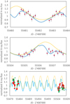 |
Fig. 1. Fit to the hard X-ray (band 4) EPIC observations, which are indicated by the red dots (with error bars only in the top panel). The uneclipsed photometric light curve from a shocked zone, which is assumed to vary proportionally to the square of the orbital separation, is shown by the orange curve. The modeled attenuated fit including eclipses of the shock zone is shown by the blue curve. Observed band 3 flux (green triangles) is included in the complete view of the fit shown in the bottom panel. |
The relative amplitude of band 4 is on the order of ±20%. The analyses by SK19 yielded for the eccentricity of the orbit e = 0.1. If we adopt that the flux from the shock zone is varying with the square of the distance between the two objects, we conclude from the observed relative variations that basically 100% of the hard X-ray emission is formed in the central shock. The variation of band 3 is similar to that of band 4, whereas the variations in the softer bands 1 and 2 are much smaller, as expected, since energy in these bands is the sum of freshly heated material close to the central shock plus previously shocked material traveling down stream and emission arising further out in the wind most likely due to global wind instabilities.
Huenemoerder et al. (2015) analyzed the light curve obtained with the Chandra X-ray Observatory during three pointings in 2013. The total count rates varied by only 5%, which is somewhat smaller but comparable to the variation of the total counts observed by XMM-Newton in 2010 which had a variation of 8%. Their finding that the variations in the full Chandra bandwidth did not correlate with the simultaneous optical variations is consistent with the notion that the soft X-rays are produced primarily in global wind structures, overwhelming the variations occurring in the localized region near the companion. A comparison of the optical variations with the hard X-ray variations might presumably have yielded a better correlation.
The fit in Fig. 1 shows two eclipses, one around the minimum of the light curve and a second near the maximum. The first of these has a duration close to half of the orbit and we attribute it to attenuation by the WR wind of the central collision zone. The effect of the wind optical depth, which is expected to be small for the hard X-ray band, is modeled by a Gaussian curve centered on the conjunction when the WR star is in front. Possible additional absorption by a trailing interaction zone is not taken into account. The strength of the eclipse is not well constrained by the observations. In Fig. 1, we have used a relatively moderate absorption of 6.4%, a value which we adapted from the absorption strength calculated from a two-component spectral fit by Skinner et al. (2002, Table 3). However, a range from almost zero absorption to absorption several factors stronger could equally well be fit because this long duration attenuation basically introduces only an offset between the uneclipsed and the eclipsed curves that is nearly constant.
We associate the second eclipse (the one which is superposed on the light curve maximum) with partial occultation by the companion of its shocked region. This eclipse is computed in the fit, with depth and duration as free parameters. Although it is better defined by the data than the one near light minimum, the observations between JD 55506.5 and 55507.5 do not cover the full eclipse duration so the fit parameters are uncertain. This has as consequence that the orbital parameters given in Table 4 (the anomalistic period between maxima, the sidereal period between eclipses, the epoch of maximum, and the epoch of conjunction) also have significant uncertainties.
The fit indicates that the duration of maximum emission is very short and in particular, shorter than the XMM-Newton exposure times. This implies that, because of the statistics needed to see a spectrum, there is always much less time (contribution) of the high hard X-ray state than of the low hard X-ray state (eclipsed). In addition the orbit solution shown in Fig. 1 reveals that no maximum is fully covered by observations and that the time of expected highest flux is within an eclipse.
4. The binary model applied to the IUE data
The IUE observations that we analyze consist of SWP spectra obtained sequentially over at least one orbital cycle in the years 1983, 1988, 1992 and 1995. The four data sets are comprised of 404 spectra.
Willis et al. (1989) analyzed the 28 SWP spectra of 1983 and remarked on their very low level of variability compared to spectra that had been acquired in the timeframe 1978–1980. A slightly higher level of variability was reported by St. -Louis et al. (1993) in a 6-day run of observations in 1988, which suggested the presence of variations on a 1 d timescale. The spectra obtained in 1992 cover ∼1.4 orbital cycles and were discussed in St. -Louis et al. (1995).
The 1995 data set was obtained over 16 consecutive days as part of the IUE-MEGA campaign (Massa et al. 1995). The spectra display clear line and continuum variability on the 3.7 d period, which were interpreted by St. -Louis et al. (1995) in terms of a global wind structure pattern which could equally well be explained with an ionized cavity around a neutron star companion or a corotating interaction region. They identified two types of line profiles in the strong emission features corresponding to approximately opposite phases in the 3.7 d period. The first, which they termed the “quiet” state, is characterized by P Cygni profiles having an absorption edge indicative of a terminal wind speed ∼1900 km s−1. In the second, termed the “high velocity” state, there is enhanced absorption extending out as far as ∼2900 km s−1 together with excess emission at lower speeds. The 1992 spectra follow the same pattern as those of 1995. However, in the 1983 and 1988 data, the high velocity state is absent.
Morel et al. (1997) revisited these IUE spectra in conjunction with a comprehensive analysis of optical spectra and photometry. They found: (a) the presence of extra emission subpeaks that travel across the emission line profiles; (b) a correlation between the strength of the emission lines and the stellar brightness; (c) a 1 day recurrence time scale for variations; (d) at maximum light there is enhanced He I absorption at high velocities; (e) the N V λ4604 P Cyg absorption component disappears as the star brightens.
4.1. Epoch 1995
We address the 1995 data set first, since it covers four of the 3.7 d cycles and thus allows a broader perspective of the variability cycles. Using Eq. (1), we find periodic flux variations on the 5–20% level in most5 of the emission bands listed in Table 2 and by factors of up to 2.5 in the P Cygni absorption bands. The variability is illustrated in Fig. 2 where the flux in three of the bands are plotted over the four orbital cycles. The times of maximum, obtained by fitting a Gaussian function to the maxima are listed in Table 3. In each cycle, the first to reach maximum are Fc1840, NIVe, NIVa, and HeIIe, followed in progression by CIVe, 1371e, FeVpsudo, and HeIIa. The average separation in time between the first and last bands to reach maximum is 0.7 d. The manner in which the flux of each band rises and declines is shown by the Chebyshev fits in Fig. 3 whose Gaussian full width at half maximum (gfwhm) range from ∼1 d to 1.6 d; that is, ≤40% of the 3.7 d cycle. We note that the N V resonance doublet does not show flux variations on the 3.7 d period.
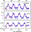 |
Fig. 2. UV flux (dots) as a function of JD-2449700 (epoch 1995) in three wavebands illustrating the periodic increase associated with periastron. Fluxes are normalized to the average value of each band. The curves show a Chebyshev 50-order polynomial fit to the measured fluxes. |
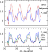 |
Fig. 3. Chebyshev 50-order polynomial fit to the UV fluxes showing the phase lag in ascending and descending intensity branches of the following bands. Top: 1371e (red), FeVpsudo (black) and Fc1840 (blue). Bottom: Fc1840 continuum (blue), NIVe (green) CIVe (red) and HeIIe (black). |
Times of maxima and dips in the IUE 1995 fluxes.
Many of the flux-weighted radial velocities obtained with Eq. (2) also display periodic variations. The semi-amplitude for the emission line RVs is ∼40 km s−1, as illustrated in Fig. 4, where the following bands are plotted: FeVpsudo, FeVIpsudo, HeIIa, and 1371e. The fourth of these is clearly in anti-phase with the first three, thus suggesting the existence of a double-line RV curve. The N V resonance doublet shows similar RV variations to those of 1371e, but the curve is considerably more noisy.
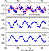 |
Fig. 4. Flux-weighted radial velocities obtained from Eq. (2), corrected for their corresponding average values, as a function of JD-2449700 of the following bands. Top: FeVpsudo (filled circle) and FeVIpsudo (open circle); middle: 1371e; bottom: HeIIa. |
Comparing Figs. 2 and 4 one can see dips in the fluxes (for example, around day 38) which coincide with the times at which the FeVpsudo RV curve crosses from negative to positive velocities. The dips are assumed to appear when a portion of the shock region is occulted by either the WR or the secondary star; that is, the dips are associated with times of conjunction.
According to the wind collision model, periastron is expected to coincide with maximum line flux. In addition, the orbital motion of the unseen companion should be evident in the RVs of high ionization lines formed near the vortex of the shock. Thus, the binary model was applied to numerous combinations of flux and radial velocity curves6. In addition to fitting these curves, the constraint was imposed that the model also fit the dips in the flux curves.
The spectral features which yield the most consistent results under the imposed constraints are 1371e and the FeVIpsudo and FeVpsudo bands7, and they provide a first set of orbital periods and initial epochs. It must be noted, however that the flux-weighted RVs give only a lower limit to the variation amplitude. This is because the bulk of the emission comes from the WR wind, which dilutes the flux-weighted RVs of the weaker shock emission. Hence, we manually measured the top of the 1371e emission and a neighboring emission at 1362 Å by fitting Gaussians. We refer to these features as G1376 and G1362, respectively. This was performed also for the absorption feature that lies at λ1324.8 Å, henceforth referred to as G1324, a relatively clean P Cygni absorption component.
The Gauss-fit RVs of both emission lines yield nearly identical RV curves with a semiamplitude ∼150 km s−1. Repeating the fitting procedure using the flux-weighted RVs of the FeV/FeVIpsudo bands (for the WR orbital motion) and the Gaussian-measured RVs of G1376 (for the companion) yields the values of the periods (anomalistic and sidereal) and corresponding initial epochs that are listed in Table 4. The fits are shown in Fig. 5. The observed variability of the 1371e shown in this figure leads us to conclude that 33% of its flux arises in the collision zone. The fit also shows that it is partially eclipsed when the WR star is in front. The best fit model parameters also indicate that the flux is weakly attenuated when the companion is in front. The RV curves are plotted as a function of sidereal phase in Fig. 6 (right).
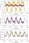 |
Fig. 5. Binary model fit to the 1995 IUE data. Top: flux-weighted mean radial velocities of FeVpsudo and FeVIpsudo (red dots), flux-weighted radial velocities of 1270e (black dots) and Gaussian measured RVs of G1376 (orange dots). The gray and blue curves are the fits to, respectively, the WR star and the less massive object. Middle: flux variations in the 1371e band (red dots) and the calculated flux variation (blue curve) that is obtained from the simultaneous fit to the RVs that are shown in the top panel. Bottom: fit to the 1995 photometric observations of Morel et al. (1997) that were obtained contemporaneously with the IUE-MEGA campaign. The mean of the u and v magnitudes are indicated by green dots. The blue curve indicates the photometric variations that were calculated with the parameters obtained by fitting the IUE data given in the two panels above. The orange shows the results of an independent fit to the photometric observations. |
Summary of Ephemerides.
The photometric observations in the visual spectral range that were obtained contemporaneously with the 1995 IUE spectra (Morel et al. 1997) were also fit with the model and are shown in Fig. 5. The resulting ephemerides are consistent with those derived from the IUE flux and radial velocity curves. However, there is a time-offset between maxima in the visual photometry and the 1371e. This offset is such that visual maxima occur ∼0.5 d earlier than the 1371e maxima, which is in the same sense as the offset between the Fc1840 continuum maximum and the 1371e band. One interpretation for this and the other time offsets is that different zones in the shock and in the neighboring outflowing wind respond differently to the changing wind density encountered around periastron. An additional factor involves the viewing angle to the portion of the companion star’s surface which is irradiated by the WR star and predicted to be significantly hotter than the opposite hemisphere (see Sect 4.5) and is expected to contribute to continuum flux when in view. From the observed variability we conclude that 19% of the optical photometric flux is associated with the collision zone.
4.2. Epoch 1992
The 1992 data set cover a little over one orbital cycle, but have a higher density of phase coverage that the 1995 data set. We applied a similar procedure as for the 1995 epoch. The fits are illustrated in Fig. A.3 and the RV curves as a function of sidereal phase are shown in Fig. 6 (left).
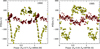 |
Fig. 6. Radial velocities as a function of sidereal phase of the G1376 emission peak measured with Gaussian fits (yellow circles) and the flux-weighted velocities of the FeVpsudo band (red circles). Phase zero corresponds to the conjunction with the WR star in front. Left: epoch 1992; right: epoch 1995. |
Except for a sharper minimum in the 1992 companion’s RV curve, the 1992 and 1995 RV curves are very similar. We explored the possibility of a higher eccentricity, e = 0.4, in 1992 which improved the RV fit (see Fig. A.4). However, such a large value for e is ruled out by the fits for the other epochs, which leads us to speculate that the sharp RV minimum may be caused by a wind effect.
4.3. Epochs 1983 and 1988
As noted previously, the 1983 and 1988 spectra display much weaker variability than present in 1992/1995. Here we focus on the 1988 data because the phase coverage in 1983 is very sparse compared to the other epochs and because the average 1983 spectrum is nearly indistinguishable from that of 1988. The flux-weighted RVs display notable variations only in bands CIVe, HeIIe, NIV], 1270e, 1270n, FeVpsudo and FeVIpsudo (see Fig. A.1), all with a very small (< 40 km s−1) semi-amplitude. Fits to the flux-weighted RVs of the two latter bands and the fluxes in 1270e yield the tentative ephemerides for this epoch listed in Table 4. Gaussian measured RVs yield somewhat larger amplitude variations in the two emission lines analyzed (G1376 and G1362) and in the G1324 absorption. The corresponding RV curves folded with the sidereal ephemeris are plotted in Fig. 7 (left). The G1324 absorption vanishes during periastron in the 1992 and 1995 epochs, for which its RVs could not be measured. At other times, however, it appears to behave similarly to what is observed in 1988, as illustrated in Fig. 7 (right) if shifted both in phase and in velocity. The significance of the phase shift is not clear. The mean velocity shift, however, could possibly be attributed to a change in the systemic velocity.
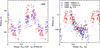 |
Fig. 7. Left: epoch 1988 Gaussian measured RVs of the G1376 emission (star) and G1324 absorption (cross) plotted as a function of sidereal orbital phase. RVs are corrected for their corresponding average values. Right: epoch 1988 RVs of G1324 (cross) unshifted in velocity but shifted by 0.5 in sidereal phase, compared to the same measurements for 1992 (square, shifted by −80 km s−1) and 1995 (triangle; shifted by −120 km s−1). The abscissa is the sidereal phase for 1992 and 1995, computed with the parameters listed in Table 4 for the corresponding epoch. |
4.4. Properties of the orbit
The fits described in the previous sections yield the anomalistic and sidereal periods PA and PS, respectively, and the precession period U as listed in Table 4. Inspection of the PA and PS values shows differences ≤0.1 d that can be accounted for by the short timespans covered by each observing campaign. Even for the 1995 epoch, which covers five orbital periods, the values of PA and PS can only be determined to two significant digits. Thus, the determined values of PS are not significantly different from 3.766 d determined by Antokhin et al. (1994) from three months of uninterupted narrow band photometry in mid February to mid May 1993, and which agrees with the sidereal period determined by SK19. We tested the sensitivity of our fits to the period by setting the sidereal period Ps = 3.766 d, and varying only the apsidal motion in the fit procedure to get the value of PA. To the eye the resulting fit does not differ from what is shown in Fig. 5 and numerically the agreement is not significantly worse based on the scatter of the measurements. Comparing in Table 4 the two entries for the ephemerides of the IUE data in 1995, provides insight into the uncertainties of the values. In particular it cannot be excluded that the sidereal period remained stable in all epochs.
The 1983 and 1988 fits suggest a much smaller inclination of the orbital plane than what we obtain of 1992 and 1995. A time-dependent variation in the orbital plane inclination is consistent with rapid apsidal motion, and could provide an explanation for the epoch-dependent spectral changes that are discussed in Sect. 5.
4.5. The nature of the close companion
The orbital parameters obtained from simultaneous fits to the Gauss-measured radial velocities of the peak G1376 and the fluxes 1371e are listed in Table 5. The amplitudes obtained from the G1376 RVs and the flux-weighted mean radial velocities of FeVpsudo and FeVIpsudo are similar for 1992 and 1995. The ratios of the velocities are 4.1 and 5.9 for 1992 and 1995, respectively. If we assume a mass of 20 M⊙ for the WR star, adopted from Schmutz (1997)8, then we obtain a mass range from 3.4 M⊙ to 4.8 M⊙ for the low-mass companion. As a WR star of 20 M⊙ stems from an even more massive star with its hydrogen rich envelope being shed, this star is only a few million years old. Thus, consulting the evolutionary calculation tables of Ekström et al. (2012) we conclude that the less massive object is likely to be a main sequence B star, the models of which give an effective temperate on the order of 15 000 K, a radius of 2.3 R⊙, and 240 L⊙. However, this star cannot be a normal B-type star.
Summary of orbit parameters.
The B-star’s atmosphere on the side that is facing the WR star is irradiated by the much more luminous WR companion. Our orbital estimates given in Table 5 yield an average distance of 0.14 AU, which in turn yields a luminosity of about 800 L⊙ incident onto the B star. The irradiance onto the B-star at the center of the irradiated surface is ∼15 times larger than the flux emitted by the unperturbed B star. Its atmosphere thus needs to compensate for the incoming radiation by adjusting its temperature and temperature gradient at optical depth τ = 2/3 to emit the additional flux. A simple black-body estimate indicates that the photosphere at the central point should look like a 30 000 K atmosphere. The optically thin zone that lies above it is dominated by the WR radiation field that has a still hotter spectral distribution and this should produce an ionization equilibrium comparable to that of the WR star. In addition to the WR radiation, the B star is subjected to the incoming supersonic flow of WR wind that collides upon the already heated atmosphere. Thus, the higher layers are formed by the shocked accreting WR wind, which is cooling down from its peak temperatures that produce the X-rays. Hence, the expectation is that the B-star surface layers are extremely hot and can produce emission lines of a similar ionization stage as those in the WR wind. It is therefore quite likely that the features we detect moving in anti-phase to the WR orbital motion are formed just above the B star’s photosphere that is facing the WR star and thus do represent the B-star’s orbital motion. This conclusion, however, requires a more detailed study of the irradiated and shocked atmosphere structure.
In low mass binaries, the response of a nondegenerate star to the irradiation from a very luminous companion has been found to significantly alter its properties. The intense radiation pressure can deform its surface (Phillips & Podsiadlowski 2002), and cause structural changes that can lead to expansion (Podsiadlowski 1991) and even an irradiation driven wind (Ruderman et al. 1989; Gayley et al. 1999). These effects can form a synergy with those caused by the incoming WR wind. For example, even a modest expansion of the B-star would increase the cross-section that is exposed to the WR radiation field as well as that which intercepts the incoming wind. Though highly speculative, such variable interactions may play a role in causing epoch-dependent variations.
4.6. The third body
The strongest evidence pointing to a third object in the system is still the rapid apsidal motion. However, changes in the systemic velocity, derived from the orbital solutions to the IUE radial velocities, suggest a possible K3 ∼ 150 km s−1 for the orbital velocity amplitude of the WR+B-star (Table 5). A similar conclusion may be derived from the shifting systemic velocity obtained from the G1324 absorption (Fig. 7) which is in the same sense and with the same amplitude as the possible K3 for the other lines.
A caveat to this interpretation lies in the possible epoch-to-epoch wind structure changes. A systematically increasing wind speed could shift the G1324 P Cyg absorption to shorter wavelengths and affect the systemic speed of other lines as well.
5. Discussion
5.1. Phase-dependent line profile variability
Significant line profile variability is present in the 1992 and 1995 data sets, as already reported by St. -Louis et al. (1995), while much lower levels of variability are present in 1983 and 1988. Orbital phase-dependent line profile variations can be an important source of uncertainty for the interpretation of the radial velocity curves, which is why we examine them in detail here.
The phase-dependent variability in the line profiles of 1992 and 1995 are nearly identical. One reason why this is the case is that, according to the ephemerides for these epochs, periastron occurs, respectively, 0.29 and 0.25 in phase after the conjunction when the WR is in front. This means that in both cases, the unseen companion is approaching the observer in its orbit at a time when the wind density at the orbital distance is largest. Hence, the excess emission is strongest, and it is blue-shifted because of the companion’s radial velocity and because there is shock-heated WR wind expanding outward with a velocity component approaching the observer.
To illustrate the above, the spectra were averaged into four sidereal phase bins: bin 1 (0.9≤ϕ≤1.1) corresponds to the WR star in front; bin 3 (0.4 ≤ ϕ ≤ 0.6) corresponds to the companion in front; bin 2 (0.2 ≤ ϕ ≤ 0.3) corresponds to the companion approaching in its orbit; and bin 4 (0.7 ≤ ϕ ≤ 0.8) corresponds to the companion receding. It is important to note that the bin 2 phase interval includes periastron. The binned 1995 spectra are plotted in Fig. 8 and show the excess emission of the bin 2 spectrum. Specifically, whereas most of the lines in the λλ1250–1350 spectral region (dominated by Fe VI transitions) have P Cyg profiles at other phases, at this phase they are filled in by emission.
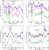 |
Fig. 8. Binned spectra of 1995 at four (sidereal) orbital phases. Low mass companion approaching (ϕS = 0.2–0.3; blue) and receding (ϕs = 0.7–0.8; red). These spectra are shifted vertically for clarity in the figure. The spectra corresponding to conjunctions are at ϕS = 0.9–1.1 (WR in front, magenta) and ϕS = 0.4–0.6 (green). Each panel illustrates a different wavelength region. The horizontal lines enclose wavelength regions defining bands that were used for flux measurements. |
The majority of blends in the λλ1250–1350 spectral region arise from transitions between excited levels of Fe VI, and in the λλ1350–1470 region from Fe V. The dominant effect is that the intrinsic WR spectrum in 1992 and 1995, consisting of P Cygni profiles in the FeV-VI region, is altered around periastron by the superposition of emissions that fill in the absorptions. Excess emission persists in the bin 3 spectrum since at this phase the unseen companion is on the near side of the WR. Contributing lines are likely the same Fe VI shifted to shorter wavelengths as they originate in outflowing shock-heated WR wind.
In addition to FeV-VI transitions, lines from even higher ionization species originating in the shock regions are expected to strengthen at periastron. For example, in the spectral regions shown in Fig. 8, one finds that the excess emission at λλ1265–1268 may include contributions from Fe VII, S IV, S V, and Si V. In λλ1322–1327 there are lines of S IV, S VI, and possibly Si IX. In λλ1330–1333 possible contributions include Si VI, O IV, S IV, Mg IV, Fe VII, Si VII.
The Fe V P Cyg absorption components in the λλ1350–1420 region are not as filled-in by emission around periastron as is the Fe VI region. It is here where a wavelength shift in the emission peaks is most evident when comparing the bin 2 and bin 4 spectra. Specifically, the line maxima at phases ∼0.2–0.3 are shifted by −350 km s−1 with respect to those of phases ∼0.7–0.8. Thus, in addition to the excess emission that extends out to −1300 km s−1, the peak emission of the associated line, near line center, shifts blueward in bin 2 with respect to the opposite phase. We interpret this emission to arise in the shock region closest to the companion.
The P Cygni profiles of the resonance and other strong lines change notably between the two periapses (bin 2 and bin 4), as already noted by St. -Louis et al. (1995) and illustrated in Fig. 9. Near periastron (bin 2, companion approaching), they have much faster blue-shifted absorption edges as well as excess emission on the blue wing at low velocity, which echoes the behavior of the excess emission in the Fe V and Fe VI lines. It is important to note, however, that the saturated portion of the absorptions (referred to as Vblack) does not change significantly.
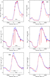 |
Fig. 9. Binned spectra at sidereal phases ϕ = 0.2–0.3 (blue) and 0.7–0.8 (red) for epochs 1992 (left) and 1995 (right), showing their very similar phase-dependent line profile variability. The abscissa is in velocity units centered on the reference wavelengths: top: N V λ1238.32; middle: C IV λ1538.20; bottom: N IV λ1718.55. The corresponding wavelength bands defined for these features and listed in Table 2 are indicated in the left panel with horizontal lines. |
An interpretation for the higher speed P Cyg absorptions around periastron is not straightforward. There is a lag between the time when the WR wind passes the companion’s orbit and the time when this material attains the fastest speed indicated by the excess absorption. This is illustrated with the integrated flow time of the WR wind, using the velocity law given by Schmutz (1997; Fig. 10). Our Fig. 10 shows that the wind velocity is 1300 km s−1 when it reaches the companion’s orbit at periastron and 1400 km s−1 at apastron, and that the flow time is 0.1–0.2 d to the companion. This is a relatively small fraction of the orbital period. However, for the material that forms the absorptions with shifts greater than 2000 km s−1 the flow time is half an orbit or longer. This means that, if the fast P Cygni absorptions that are observed at periastron arise in the WR wind, the material causing them could have left the star at the time of apastron or even at around the time of the previous periastron. Alternatively, the high speeds may arise in material that is accelerated by shocks, instead of representing a global wind velocity. The accelerating mechanism, however, would have to affect both the approaching and receding wind, since excess emission in the He II λ1640 red wing is also present at the same time as the excess blue absorption. Furthermore, there is a correlated change in the shape of the N IV λ1718 which also points to additional absorption at faster speeds.
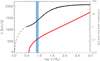 |
Fig. 10. Integrated flow time of the wind (axis on the right) from the calculated velocity law shown in Fig. 10 of Schmutz (1997). The velocity law is shown in black and the cumulative flow time of the wind in red, starting at the photosphere, where the wind optical depth is τ = 1. This corresponds to the model radius 3 R* (= 10 R⊙). The blue rectangle encloses the distance between the two stars at periastron, 26 R⊙ (= 0.87 log10(r/R*)), and apastron, 32 R⊙ (= 0.96 log10(r/R*)). |
The most notable aspect of the 1988 spectra is their significantly weaker variability compared to the later epochs. This is perplexing, but may potentially be understood as a consequence of a slower WR wind during this epoch, as implied by the P Cyg profiles as discussed below.
Also noteworthy is the fact that most of the 1988 spectral features are very similar to those in the apastron (bin 4) spectra in 1992 and 1995. The similarity is illustrated in Fig. 11, where we compare the average 1988 spectra at RV minimum and at maximum with the apastron spectrum of 1992. The one major difference between these spectra is in the resonance lines, which in 1988 have less extended P Cygni absorptions than in the later epochs. This is further discussed in Sect. 5.2.
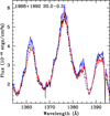 |
Fig. 11. Line profiles in the average spectra of 1988 at minimum RV (blue) and maximum RV (red) (see Fig. 7, left) illustrating their similarity to the apastron spectrum of 1992 (dash). |
The 1988 spectra display a phase-dependent variation in the flux ratio Fe VI/Fe V as illustrated in Fig. 12. The ratio rises toward maximum just prior to the time of periastron. A similar ionization variation is not seen in the 1992 and 1995 epochs, possibly because the shock is stronger and instead of FeV-VI, even higher ionization stages dominate.
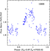 |
Fig. 12. Flux ratio FeVIpsudo/FeVpsudo plotted as a function of sidereal phase in the 1988 data, with periastron at ϕS ∼ 0. |
5.2. Epoch to epoch variations
The epoch-dependent changes are quantified in Table A.1 where we list for the 1983, 1988, 1992 and 1995 epochs the average over all orbital phases flux, flux-weighted velocity, and the corresponding standard deviations for the spectral bands that were measured. Inspection of this table discloses two notable trends. The first trend is one in which the continuum flux in the λλ1828–1845 band increased over time. Specifically, its value with respect to that of 1995 was 0.88, 0.90, and 0.99 for 1983, 1988 and 1992, respectively. A similar result was also reported in Morel et al. (1997).
The second trend is that the degree of variability over the 22 bands that were measured also increased over time. The flux standard deviations of Epochs 1983, 1988 and 1992 are, respectively, 0.33, 0.62 and 0.86 that of 1995. Similarly, the corresponding velocity standard deviations are 0.53, 0.68, and 0.95.
As mentioned above, the 1983 and 1988 spectra are very similar to the bin 4 (around apastron) spectra of 1992 and 1995. Thus, the increase over time in the fluxes and their standard deviations are dominated by the blue-shifted emissions that appear in the bin 2 (periastron) spectra of the later years.
Comparing the bin 4 (apastron) spectra of 1992 and 1995 with the average spectra of 1983 and 1988 discloses a single difference: the maximum extent of the N V and C IV P Cygni absorptions. These resonance lines are shown in Fig. 13. In the later epochs, the entire P Cygni absorption component, including the saturated portion of the profile, is stretched towards shorter wavelengths. The extent of their blue edge increases from −2400 km s−1 in 1983 and 1988 to −2500 km s−1 in 1992 and then to −2680 km s−1 in 1995. The corresponding Vblack is −1840 km s−1 (1983 and 1988), −2100 km s−1 (1992) and −2300 km s−1 (1995). Such an effect is not present in He II nor N IV, which arise from excited transitions. Thus, the resonance lines suggest the presence in 1992 and 1995 of low density material that lies along the line-of sight to the WR core and that is accelerated to faster speeds than present in the earlier epochs. The slight emission increase in N IV] λ1486 may be another manifestation of the same phenomenon. However, the N IV λ1718 P Cyg absorption shows only a weak change from epoch to epoch. This line is formed nearer to to the base of the wind than the resonance lines, and it has a smaller opacity so it is less sensitive to processes that occur far out in the wind.
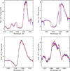 |
Fig. 13. Line profiles of N V and C IV in the average spectrum of HD 50896 in 1988 (black) and in the binned spectra at apastron in 1992 (red) and 1995 (blue dash) showing a systematic increase in the extent of the P Cygni resonance line absorptions which is less evident in N IV λ1718 with no width change in N IV] λ1486. |
We conclude by speculating that the faster wind speed in the later epochs results in a stronger feedback in the shock-heated region near the companion which, in turn causes a larger degree of orbital phase-dependent variability.
5.3. CIRs, wind-wind collisions and periastron effects
Some of the observed variations in EZ CMa and other presumed single sources with strong winds has often been attributed to corotating interaction regions (CIRs, Mullan 1984). These are assumed to arise in an aspherical stellar wind or in active zones near the stellar photosphere of a rotating single star. As the perturbations propagate outward, they form a spiral density structure that is embedded in the WR wind (Carlos-Leblanc et al. 2019). Qualitatively, this spiral structure may be analogous to that which arises from a wind-wind collision and its trailing shock region that propagates outward (Parkin & Pittard 2008; Parkin et al. 2009). The dynamics and detailed structure of the spiral depend on the orbital parameters and mass-loss properties of the two stars.
The line profile variability expected from a wind-wind collision region was modeled by Ignace et al. (2009) for the case of forbidden emission lines. Although their model is applied to a WR+OB binary, their predicted variations are qualitatively similar to those that were reported by Firmani et al. (1980) for the He II λ 4686 emission line; that is, it changes from a flat-top to a peak that is either centered or on the blue or the red side of the underlying broad emission. Thus, one could speculate that the high ionization UV lines describe the processes occurring near the companion while the optical lower ionization lines describe those that occur further downstream from the shock.
Associating the CIR phenomenon with an origin in the binary companion would help solve the question surrounding the trigger for the CIR formation in EZ CMa. However, a quantitative analysis is required in order to test whether the observational diagnostics of CIR-like spirals produced in a colliding wind binary are similar to those in assumed rotating single stars.
Interaction effects play a role in all close binary systems and particularly so when one or both possess a stellar wind. In addition to eclipse, occultation and wind collision effects, additional phase-dependent phenomena arise when the orbit is eccentric. In addition to the variations in the wind collision strength discussed in this paper, another type of interaction effect is the tidal excitation of oscillations that are triggered by periastron passage in an eccentric binary (Kumar et al. 1995; Moreno & Koenigsberger 1999; Welsh et al. 2011; Guo et al. 2020). Although the eccentricity of EZ CMa is not as large as that of binaries in which such oscillations have been observed, the theory predicts their existence. Pulsations have long been suspected to contribute towards enhancing mass-loss rates in massive stars (Townsend et al. 2007). This raises the question of the role that tidally excited oscillations may play in producing a structured stellar wind, particularly in the orbital plane. For example, one may speculate that the larger tidal perturbation amplitude at periastron leads to a structured wind with alternating slower and faster shells, with the latter catching up with and shocking the former.
A final question of potential interest concerns the amount of B-star material that might be ablated by the combined effect of irradiation and wind collision. The outflowing shocked WR wind would then carry H-rich material it has “lifted” from the B-star, leading to a mix of chemical compositions in the wind.
6. Conclusions
We analyzed X-ray and UV observational data sets that were obtained during 5 different epochs between 1983 and 2010 with the aim of further testing the eccentric binary model for EZ CMa that was proposed by SK19 and with the objective of constraining the properties of the low-mass companion. In this model, the WR wind is assumed to collide with the low-mass companion forming a very hot and highly ionized region which gives rise to hard X-rays and emission lines.
The observed flux variability in the XMM-Newton hard X-ray bands is explained by a model in which the energy deposited in the shock is proportional to the wind density at the shock location. The modulation by 0.1 eccentricity with variations proportional 1/d2 explains what is observed; that is, ±20% modulation. In addition, we find that the predicted time over which the emission maximum occurs is shorter than typical exposure times and that the time when the emission is maximum (that is, at periastron) coincided in these data with an eclipse. Hence, the phase with the hardest emission may not yet have been observed.
The extensive sets of IUE observations allow a detailed radial velocity analysis which shows that the strong WR emission lines follow a periodic RV curve with a semi-amplitude K1 ∼ 30 km s−1 in 1992 and 1995, and that a second set of weaker emissions move in an anti-phase RV curve with K2 ∼ 150 km s−1. The simultaneous model fit to the RVs and the light curve yields the orbital elements for each epoch. Adopting a Wolf-Rayet mass M1 ∼ 20 M⊙ leads to M2 ∼ 3−5 M⊙ which, given the age of the WR star, corresponds to a late B-type star (Silaj et al. 2014). We argue, however, that it is unlikely to be a normal B-type star because of the large incoming radiative flux from the WR, the additional heating by the shock-produced X-rays, and the accretion of impinging WR wind material. The combined effect of these processes can significantly alter the B-star envelope structure (Beer & Podsiadlowski 2002, and references therein) and we speculate that it may lead to the ablation of H-rich B-star material which is then carried away by the WR wind.
We speculate that as the mixture of shocked WR wind that flows past the B-star and the ablated B-star material expands outward, it forms a spiral structure that may be interpreted as the corotating interaction regions that have been modeled in previous studies (Ignace et al. 2013).
Considerable orbital-phase dependent variations are observed in the UV spectral line profiles during 1992 and 1995, as already discussed in St. -Louis et al. (1995). We find that the high velocity state that was identified by these authors corresponds to periastron passage, when the shock-induced line emission is strongest and which occurs in these epochs at the quadrature when the companion is approaching us. We are unable to find a satisfactory explanation for the peculiarly extended P Cygni absorption edges that appear in all the strong lines during this high state.
A similar high state is absent in the 1988 IUE spectra. All the spectral features of this epoch are nearly identical to the low state spectra of 1992 and 1995, with the exception of the faster wind speed in the latter two epochs as deduced from the saturated portion of resonance P Cyg absorptions. This suggests that the weaker phase-dependent variability in 1988 may be due to a slower WR wind speed which, in turn, would produce a weaker shock region near the companion.
The rapidly precessing argument of periastron deduced by SK19 implies the presence of a third object in the system. The systemic velocities obtained from the orbital solutions of the four IUE epochs differ by ∼200 km s−1, which would be consistent with an orbit of the WR (+B-type companion) around the third object. However, many more observation epochs are needed before this result can be confirmed.
Although many questions remain unanswered, we consider that the anti-phase RV variations of two emission components and the simultaneous fit to the RVs and the light curve are concrete evidence in favor of the binary nature of EZ Canis Majoris. The assumption that the emission from the shock-heated region traces the orbit of the companion is less certain, given the changing shock strength over the orbital cycle combined with the possible ablation of the companion’s envelope, questions requiring further investigation.
Available at: http://sdc.cab.inta-csic.es/ines/index2.html
It has been pointed out by an anonymous referee that Eq. (10) in Stevens et al. (1992) implies that the distance dependence of the X-ray luminosity should be linear. The assumption of the cited equation is that the geometry of the colliding winds is scale-free, so the volume of shock-heated gas scales with the distance to the power of 3. We note that in the case of EZ CMa the expected scenario is not that of a wind-wind collision but that of a wind colliding with a main sequence star. Thus, we anticipate that the hydrodynamic simulations of Ruffert (1994) for wind accretions are more adequate to guide the expectations. Model FL of Ruffert (1994) might represent the best match, in which the size of the shock region is given by the size of the star. The input energy to the shocked material is then proportional to the density of the impacting wind, which scales with d−2.
Variable features are plotted in Appendix A.
There are more recent determination of the stellar parameters of EZ CMa, such as, for example, Hamann et al. (2019). These analyses yield stellar parameters that can be considered consistent regarding the luminosity and thus, yielding a mass on the order as assumed here. However, no recent analyses has been done in such detail as Schmutz (1997), who has calculated as part of the spectroscopic analysis the velocity law of the mass loss consistently with the radiation field and the ionization structure.
Acknowledgments
This paper is based on INES data from the IUE satellite. GK thanks Ken Gayley for helpful discussions and the Indiana University Astronomy Department for hosting a visit during which much of this paper was completed, and acknowledges support from CONACYT grant 252499 and UNAM/PAPIIT grant IN103619.
References
- Antokhin, I., Bertrand, J.-F., Lamontagne, R., & Moffat, A. F. J. 1994, AJ, 107, 2179 [NASA ADS] [CrossRef] [Google Scholar]
- Beer, M. E., & Podsiadlowski, P. 2002, in Irradiation Effects in Compact Binaries, eds. C. A. Tout, & W. van Hamme, ASP Conf. Ser., 279, 253 [NASA ADS] [Google Scholar]
- Carlos-Leblanc, D., St-Louis, N., Bjorkman, J. E., & Ignace, R. 2019, MNRAS, 489, 2873 [NASA ADS] [CrossRef] [Google Scholar]
- Drissen, L., Robert, C., Lamontagne, R., et al. 1989, ApJ, 343, 426 [NASA ADS] [CrossRef] [Google Scholar]
- Duijsens, M. F. J., van der Hucht, K. A., van Genderen, A. M., et al. 1996, A&AS, 119, 37 [NASA ADS] [CrossRef] [EDP Sciences] [Google Scholar]
- Ekström, S., Georgy, C., Eggenberger, P., et al. 2012, A&A, 537, A146 [NASA ADS] [CrossRef] [EDP Sciences] [Google Scholar]
- Firmani, C., Koenigsberger, G., Bisiacchi, G. F., Ruiz, E., & Solar, A. 1978, Mem. Soc. Astron. It., 49, 453 [NASA ADS] [Google Scholar]
- Firmani, C., Koenigsberger, G., Bisiacchi, G. F., Moffat, A. F. J., & Isserstedt, J. 1980, ApJ, 239, 607 [NASA ADS] [CrossRef] [Google Scholar]
- Gayley, K. G., Owocki, S. P., & Cranmer, S. R. 1999, ApJ, 513, 442 [NASA ADS] [CrossRef] [Google Scholar]
- Georgiev, L. N., Koenigsberger, G., Ivanov, M. M., St.-Louis, N., & Cardona, O. 1999, A&A, 347, 583 [NASA ADS] [Google Scholar]
- Guo, Z., Shporer, A., Hambleton, K., & Isaacson, H. 2020, ApJ, 888, 95 [CrossRef] [Google Scholar]
- Hamann, W. R., Gräfener, G., Liermann, A., et al. 2019, A&A, 625, A57 [NASA ADS] [CrossRef] [EDP Sciences] [Google Scholar]
- Huenemoerder, D. P., Gayley, K. G., Hamann, W. R., et al. 2015, ApJ, 815, 29 [NASA ADS] [CrossRef] [Google Scholar]
- Ignace, R., Bessey, R., & Price, C. S. 2009, MNRAS, 395, 962 [NASA ADS] [CrossRef] [Google Scholar]
- Ignace, R., Gayley, K. G., Hamann, W. R., et al. 2013, ApJ, 775, 29 [NASA ADS] [CrossRef] [Google Scholar]
- Kuhi, L. V. 1967, PASP, 79, 57 [NASA ADS] [CrossRef] [EDP Sciences] [Google Scholar]
- Kumar, P., Ao, C. O., & Quataert, E. J. 1995, ApJ, 449, 294 [NASA ADS] [CrossRef] [Google Scholar]
- Lamberts, A., Millour, F., Liermann, A., et al. 2017, MNRAS, 468, 2655 [NASA ADS] [CrossRef] [Google Scholar]
- Lindgren, H., Lundstrom, I., & Stenholm, B. 1975, A&A, 44, 219 [NASA ADS] [Google Scholar]
- Massa, D., Fullerton, A. W., Nichols, J. S., et al. 1995, ApJ, 452, L53 [NASA ADS] [Google Scholar]
- Moffat, A. F. J., St-Louis, N., Carlos-Leblanc, D., et al. in 3rd BRITE Science Conference, eds. G. A. Wade, D. Baade, J. A. Guzik, et al., 8, 37 [Google Scholar]
- Morel, T., St-Louis, N., & Marchenko, S. V. 1997, ApJ, 482, 470 [NASA ADS] [CrossRef] [Google Scholar]
- Moreno, E., & Koenigsberger, G. 1999, Rev. Mex. Astron. Astrofis., 35, 157 [NASA ADS] [Google Scholar]
- Mullan, D. J. 1984, ApJ, 283, 303 [NASA ADS] [CrossRef] [Google Scholar]
- Oskinova, L. M., Gayley, K. G., Hamann, W. R., et al. 2012, ApJ, 747, L25 [NASA ADS] [CrossRef] [Google Scholar]
- Parkin, E. R., & Pittard, J. M. 2008, MNRAS, 388, 1047 [NASA ADS] [CrossRef] [Google Scholar]
- Parkin, E. R., Pittard, J. M., Corcoran, M. F., Hamaguchi, K., & Stevens, I. R. 2009, MNRAS, 394, 1758 [NASA ADS] [CrossRef] [Google Scholar]
- Phillips, S. N., & Podsiadlowski, P. 2002, MNRAS, 337, 431 [NASA ADS] [CrossRef] [Google Scholar]
- Podsiadlowski, P. 1991, Nature, 350, 136 [NASA ADS] [CrossRef] [Google Scholar]
- Rate, G., & Crowther, P. A. 2020, MNRAS, 493, 1512 [CrossRef] [Google Scholar]
- Richardson, N. D., Russell, C. M. P., St-Jean, L., et al. 2017, MNRAS, 471, 2715 [NASA ADS] [CrossRef] [Google Scholar]
- Robert, C., Moffat, A. F. J., Drissen, L., et al. 1992, ApJ, 397, 277 [NASA ADS] [CrossRef] [Google Scholar]
- Ross, L. W. 1961, PASP, 73, 354 [NASA ADS] [CrossRef] [Google Scholar]
- Ruderman, M., Shaham, J., & Tavani, M. 1989, ApJ, 336, 507 [NASA ADS] [CrossRef] [Google Scholar]
- Ruffert, M. 1994, A&AS, 106, 505 [NASA ADS] [Google Scholar]
- Schmidt, G. D. 1974, PASP, 86, 767 [NASA ADS] [CrossRef] [Google Scholar]
- Schmutz, W. 1997, A&A, 321, 268 [NASA ADS] [Google Scholar]
- Schmutz, W., & Koenigsberger, G. 2019, A&A, 624, L3 [NASA ADS] [CrossRef] [EDP Sciences] [Google Scholar]
- Silaj, J., Jones, C. E., Sigut, T. A. A., & Tycner, C. 2014, ApJ, 795, 82 [NASA ADS] [CrossRef] [Google Scholar]
- Skinner, S. L., Zhekov, S. A., Güdel, M., & Schmutz, W. 2002, ApJ, 579, 764 [NASA ADS] [CrossRef] [Google Scholar]
- St. -Louis, N., Howarth, I. D., Willis, A. J., et al. 1993, A&A, 267, 447 [Google Scholar]
- St. -Louis, N., Dalton, M. J., Marchenko, S. V., Moffat, A. F. J., & Willis, A. J. 1995, ApJ, 452, L57 [NASA ADS] [CrossRef] [Google Scholar]
- Stevens, I. R., Blondin, J. M., & Pollock, A. M. T. 1992, ApJ, 386, 265 [NASA ADS] [CrossRef] [Google Scholar]
- Toalá, J. A., Guerrero, M. A., Chu, Y. H., et al. 2012, ApJ, 755, 77 [NASA ADS] [CrossRef] [Google Scholar]
- Townsend, R. 2007, Am. Inst. Phys. Conf. Ser., 948, 345 [NASA ADS] [Google Scholar]
- van den Heuvel, E. P. J. 1976, IAU Symp., 73, 35 [Google Scholar]
- van der Hucht, K. A. 2001, New A Rev., 45, 135 [CrossRef] [Google Scholar]
- Welsh, W. F., Orosz, J. A., Aerts, C., et al. 2011, ApJS, 197, 4 [NASA ADS] [CrossRef] [Google Scholar]
- Willis, A. J., Howarth, I. D., Smith, L. J., Garmany, C. D., & Conti, P. S. 1989, A&AS, 77, 269 [Google Scholar]
- Willis, A. J., Schild, H., Howarth, I. D., & Stevens, I. R. 1994, Ap&SS, 221, 321 [CrossRef] [Google Scholar]
- Wilson, O. C. 1948, PASP, 60, 383 [NASA ADS] [CrossRef] [Google Scholar]
Appendix A: Complementary information
Average flux and velocity values for each IUE wavelength band measured for epochs 1983, 1988, 1992, and 1995.
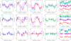 |
Fig. A.1. Velocities of lines in IUE spectra folded in phase with (PS, TS) as listed in Table 4. First row: set 1995; second row: set 1992; third row: set 1988. The spectral features that are plotted are labeled in the first row according to the naming convention given in Table A.1 (Col. 3). They correspond to the following: Col. 1: 1270e (black), HeIIr (magenta), FeVpsudo (cyan); Col. 2: HeIIa (red), NIVa (blue); Col. 3: 1226n (magenta), 1371e (cyan), HeIIb (red); Col. 4: NIVe (blue), NVe (green); Col. 5: NIVnn (black), NIVn (magenta), CIVe+35 km s−1 (cyan), HeIIe +35 km s−1 (blue), NIV]+35 km s−1 (green), 1270n-35 km s−1 (red). |
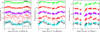 |
Fig. A.2. UV fluxes as a function of orbital phase for the epochs 1995 (left), 1992 (middle) and 1988 (right). Each line flux is normalized by the average value of the line for the given epoch. The significantly weaker modulation in 1988 compared to 1992 and 1995 is evident, as is the large cycle-to-cycle dispersion over time in the N V emission flux of 1995. |
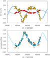 |
Fig. A.3. Fit to the 1992 (red dots) and G1376 RVs (orange with black circle) (top panel) and the fluxes in the 1371e-band (bottom panel). |
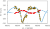 |
Fig. A.4. Same as Fig. A.3, but here is the fit to the 1992 G1376 RVs (orange with black circle) with an eccentricity e = 0.4. |
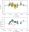 |
Fig. A.5. Fit to the 1988 IUE FeV+FeVI (red dots) and Gaussian-measured RVs (yellow with black circle) (top panel) and the fluxes in FeVIpsudo 1270-band and (bottom panel). |
All Tables
Average flux and velocity values for each IUE wavelength band measured for epochs 1983, 1988, 1992, and 1995.
All Figures
|
Fig. 1. Fit to the hard X-ray (band 4) EPIC observations, which are indicated by the red dots (with error bars only in the top panel). The uneclipsed photometric light curve from a shocked zone, which is assumed to vary proportionally to the square of the orbital separation, is shown by the orange curve. The modeled attenuated fit including eclipses of the shock zone is shown by the blue curve. Observed band 3 flux (green triangles) is included in the complete view of the fit shown in the bottom panel. |
| In the text | |
|
Fig. 2. UV flux (dots) as a function of JD-2449700 (epoch 1995) in three wavebands illustrating the periodic increase associated with periastron. Fluxes are normalized to the average value of each band. The curves show a Chebyshev 50-order polynomial fit to the measured fluxes. |
| In the text | |
|
Fig. 3. Chebyshev 50-order polynomial fit to the UV fluxes showing the phase lag in ascending and descending intensity branches of the following bands. Top: 1371e (red), FeVpsudo (black) and Fc1840 (blue). Bottom: Fc1840 continuum (blue), NIVe (green) CIVe (red) and HeIIe (black). |
| In the text | |
|
Fig. 4. Flux-weighted radial velocities obtained from Eq. (2), corrected for their corresponding average values, as a function of JD-2449700 of the following bands. Top: FeVpsudo (filled circle) and FeVIpsudo (open circle); middle: 1371e; bottom: HeIIa. |
| In the text | |
|
Fig. 5. Binary model fit to the 1995 IUE data. Top: flux-weighted mean radial velocities of FeVpsudo and FeVIpsudo (red dots), flux-weighted radial velocities of 1270e (black dots) and Gaussian measured RVs of G1376 (orange dots). The gray and blue curves are the fits to, respectively, the WR star and the less massive object. Middle: flux variations in the 1371e band (red dots) and the calculated flux variation (blue curve) that is obtained from the simultaneous fit to the RVs that are shown in the top panel. Bottom: fit to the 1995 photometric observations of Morel et al. (1997) that were obtained contemporaneously with the IUE-MEGA campaign. The mean of the u and v magnitudes are indicated by green dots. The blue curve indicates the photometric variations that were calculated with the parameters obtained by fitting the IUE data given in the two panels above. The orange shows the results of an independent fit to the photometric observations. |
| In the text | |
|
Fig. 6. Radial velocities as a function of sidereal phase of the G1376 emission peak measured with Gaussian fits (yellow circles) and the flux-weighted velocities of the FeVpsudo band (red circles). Phase zero corresponds to the conjunction with the WR star in front. Left: epoch 1992; right: epoch 1995. |
| In the text | |
|
Fig. 7. Left: epoch 1988 Gaussian measured RVs of the G1376 emission (star) and G1324 absorption (cross) plotted as a function of sidereal orbital phase. RVs are corrected for their corresponding average values. Right: epoch 1988 RVs of G1324 (cross) unshifted in velocity but shifted by 0.5 in sidereal phase, compared to the same measurements for 1992 (square, shifted by −80 km s−1) and 1995 (triangle; shifted by −120 km s−1). The abscissa is the sidereal phase for 1992 and 1995, computed with the parameters listed in Table 4 for the corresponding epoch. |
| In the text | |
|
Fig. 8. Binned spectra of 1995 at four (sidereal) orbital phases. Low mass companion approaching (ϕS = 0.2–0.3; blue) and receding (ϕs = 0.7–0.8; red). These spectra are shifted vertically for clarity in the figure. The spectra corresponding to conjunctions are at ϕS = 0.9–1.1 (WR in front, magenta) and ϕS = 0.4–0.6 (green). Each panel illustrates a different wavelength region. The horizontal lines enclose wavelength regions defining bands that were used for flux measurements. |
| In the text | |
|
Fig. 9. Binned spectra at sidereal phases ϕ = 0.2–0.3 (blue) and 0.7–0.8 (red) for epochs 1992 (left) and 1995 (right), showing their very similar phase-dependent line profile variability. The abscissa is in velocity units centered on the reference wavelengths: top: N V λ1238.32; middle: C IV λ1538.20; bottom: N IV λ1718.55. The corresponding wavelength bands defined for these features and listed in Table 2 are indicated in the left panel with horizontal lines. |
| In the text | |
|
Fig. 10. Integrated flow time of the wind (axis on the right) from the calculated velocity law shown in Fig. 10 of Schmutz (1997). The velocity law is shown in black and the cumulative flow time of the wind in red, starting at the photosphere, where the wind optical depth is τ = 1. This corresponds to the model radius 3 R* (= 10 R⊙). The blue rectangle encloses the distance between the two stars at periastron, 26 R⊙ (= 0.87 log10(r/R*)), and apastron, 32 R⊙ (= 0.96 log10(r/R*)). |
| In the text | |
|
Fig. 11. Line profiles in the average spectra of 1988 at minimum RV (blue) and maximum RV (red) (see Fig. 7, left) illustrating their similarity to the apastron spectrum of 1992 (dash). |
| In the text | |
|
Fig. 12. Flux ratio FeVIpsudo/FeVpsudo plotted as a function of sidereal phase in the 1988 data, with periastron at ϕS ∼ 0. |
| In the text | |
|
Fig. 13. Line profiles of N V and C IV in the average spectrum of HD 50896 in 1988 (black) and in the binned spectra at apastron in 1992 (red) and 1995 (blue dash) showing a systematic increase in the extent of the P Cygni resonance line absorptions which is less evident in N IV λ1718 with no width change in N IV] λ1486. |
| In the text | |
|
Fig. A.1. Velocities of lines in IUE spectra folded in phase with (PS, TS) as listed in Table 4. First row: set 1995; second row: set 1992; third row: set 1988. The spectral features that are plotted are labeled in the first row according to the naming convention given in Table A.1 (Col. 3). They correspond to the following: Col. 1: 1270e (black), HeIIr (magenta), FeVpsudo (cyan); Col. 2: HeIIa (red), NIVa (blue); Col. 3: 1226n (magenta), 1371e (cyan), HeIIb (red); Col. 4: NIVe (blue), NVe (green); Col. 5: NIVnn (black), NIVn (magenta), CIVe+35 km s−1 (cyan), HeIIe +35 km s−1 (blue), NIV]+35 km s−1 (green), 1270n-35 km s−1 (red). |
| In the text | |
|
Fig. A.2. UV fluxes as a function of orbital phase for the epochs 1995 (left), 1992 (middle) and 1988 (right). Each line flux is normalized by the average value of the line for the given epoch. The significantly weaker modulation in 1988 compared to 1992 and 1995 is evident, as is the large cycle-to-cycle dispersion over time in the N V emission flux of 1995. |
| In the text | |
|
Fig. A.3. Fit to the 1992 (red dots) and G1376 RVs (orange with black circle) (top panel) and the fluxes in the 1371e-band (bottom panel). |
| In the text | |
|
Fig. A.4. Same as Fig. A.3, but here is the fit to the 1992 G1376 RVs (orange with black circle) with an eccentricity e = 0.4. |
| In the text | |
|
Fig. A.5. Fit to the 1988 IUE FeV+FeVI (red dots) and Gaussian-measured RVs (yellow with black circle) (top panel) and the fluxes in FeVIpsudo 1270-band and (bottom panel). |
| In the text | |
Current usage metrics show cumulative count of Article Views (full-text article views including HTML views, PDF and ePub downloads, according to the available data) and Abstracts Views on Vision4Press platform.
Data correspond to usage on the plateform after 2015. The current usage metrics is available 48-96 hours after online publication and is updated daily on week days.
Initial download of the metrics may take a while.