| Issue |
A&A
Volume 638, June 2020
|
|
|---|---|---|
| Article Number | A75 | |
| Number of page(s) | 13 | |
| Section | Cosmology (including clusters of galaxies) | |
| DOI | https://doi.org/10.1051/0004-6361/201937313 | |
| Published online | 15 June 2020 | |
Filament profiles from WISExSCOS galaxies as probes of the impact of environmental effects
1
Institut d’Astrophysique Spatiale, CNRS, Université Paris-Sud, Bâtiment 121, Orsay, France
e-mail: This email address is being protected from spambots. You need JavaScript enabled to view it.
2
LERMA, Observatoire de Paris, PSL Research University, CNRS, Sorbonne Universités, UPMC Univ. Paris 06, 75014 Paris, France
Received:
13
December
2019
Accepted:
19
March
2020
Abstract
The role played by large-scale structures in galaxy evolution is not very well understood yet. In this study, we investigated properties of galaxies in the range 0.1 < z < 0.3 from a value-added version of the WISExSCOS catalogue around cosmic filaments detected with DisPerSE. We fitted a profile of galaxy over-density around cosmic filaments and found a typical radius of rm = 7.5 ± 0.2 Mpc. We measured an excess of passive galaxies near to the spine of the filament that was higher than the excess of transitioning and active galaxies. We also detected star formation rates (SFR) and stellar mass (M⋆) gradients pointing towards the spine of the filament. We investigated this result and found an M⋆ gradient for each type of galaxy, that is active, transitioning, and passive; we found a positive SFR gradient for passive galaxies. We also linked the galaxy properties and gas content in the cosmic web. To do so, we investigated the quiescent fraction fQ profile of galaxies around the cosmic filaments. Based on recent studies about the effect of the gas and the cosmic web on galaxy properties, we modelled fQ with a β model of gas pressure. The slope obtained in this work, β = 0.54 ± 0.18, is compatible with the scenario of projected isothermal gas in hydrostatic equilibrium (β = 2/3) and with the profiles of gas fitted in Sunyaev-Zel’dovich data from the Planck satellite.
Key words: methods: data analysis / galaxies: statistics / cosmology: observations / large-scale structure of Universe
© V. Bonjean et al. 2020
 Open Access article, published by EDP Sciences, under the terms of the Creative Commons Attribution License (https://creativecommons.org/licenses/by/4.0), which permits unrestricted use, distribution, and reproduction in any medium, provided the original work is properly cited.
1. Introduction
The matter distribution in the Universe is very non-linear and very complex, structured into a cosmic web composed of voids, walls, filaments, and nodes (e.g. Zel’Dovich 1970; Bond et al. 1996; Libeskind et al. 2018). Understanding the evolution and physical properties of the matter around the largest scale structures remains one of the main challenges in observational and theoretical cosmology.
Nowadays, numerical simulations such as Millenium (Springel 2005), Illustris-TNG (Springel et al. 2018), Horizon-AGN (Dubois et al. 2014), or Magneticum (Hirschmann et al. 2014) allow us to trace and characterise all the matter (i.e. dark matter, hot gas, cold gas, and galaxies) of the large-scale Universe. Among the different structures of the cosmic web, the objects that are the easiest to detect and characterise are those with the highest densities (i.e. the nodes), where the galaxy clusters lay. The average properties of these objects are known (e.g. Kravtsov & Borgani 2012; Bykov et al. 2015; Walker et al. 2019) thanks to numerical simulations as well as actual observations of galaxies in the optical and near-infrared, hot gas via the Sunyaev-Zel’dovich effect (SZ; Sunyaev & Zeldovich 1970, 1972) and in X-rays, and dark matter via gravitational lensing. As a matter of fact, dark matter and hot gas universal density profiles have already been derived around these structures (e.g. Nagai et al. 2007; Arnaud et al. 2010; Planck Collaboration Int. V 2013; Bartalucci et al. 2017; Ghirardini et al. 2019), and global picture of the distribution and the properties (such as the SFR and stellar mass) of galaxies that fall into their gravitational potential has already been drawn (e.g. Mahajan & Raychaudhury 2009; Mahajan et al. 2011; Baxter et al. 2017; Chang et al. 2018; Adhikari et al. 2019; Pintos-Castro et al. 2019).
While galaxy clusters are relatively easy to detect, study, and characterise, other cosmic web structures, such as cosmic filaments, are not easily defined because of their low densities. No global picture such as that drawn for galaxy clusters has been derived yet, and even the definition of cosmic filaments is still arguable since it depends on the way they are detected. Several methods have been proposed to detect the cosmic filaments: for example Bisous (Tempel et al. 2016), DisPerSE1 (Sousbie 2011), NEXUS+ (Cautun et al. 2013), or very recently T-ReX2 (Bonnaire et al. 2020). Each of these methods has advantages and disadvantages, making it difficult to compare them (see Libeskind et al. 2018 for a review or Bonnaire et al. 2020). Despite this, recent studies have used those methods to investigate the physical properties of the matter (dark matter, gas, or galaxies) in filaments in numerical simulations (e.g. Colberg et al. 2005; Dolag et al. 2006; Aragón-Calvo et al. 2010; Cautun et al. 2014; Gheller et al. 2015, 2016; Martizzi et al. 2019; Gheller & Vazza 2019; Galárraga-Espinosa et al. 2020). Indeed, studying gas is only possible in numerical simulations. The hot gas around cosmic filaments is very hard to detect either in SZ or in X-rays because of its low density and low temperature. Hot gas is only accessible in a few exceptional objects such as the galaxy cluster pair A399-A401 (e.g. Fujita et al. 1996, 2008; Sakelliou & Ponman 2004; Akamatsu et al. 2017; Bonjean et al. 2018), the galaxy cluster A2744 (Eckert et al. 2015), or between the two clusters A3391 and A3395 (Planck Collaboration Int. VIII 2013, recently observed in X-rays with eROSITA). Alternatively, some studies have used the stacking around the highest density regions in between galaxy cluster pairs (Tanimura et al. 2019a; de Graaff et al. 2019) or inside super-clusters (Tanimura et al. 2019b) to detect the densest parts of the gas in the filaments around clusters. The first statistical study of the hot gas using the SZ effect around cosmic filaments was performed in Tanimura et al. (2020).
Galaxies around cosmic filaments, which are easier to detect, have recently started to be extensively studied in the following surveys: the Sloan Digital Sky Survey (SDSS) in 3D (e.g. Martínez et al. 2016; Chen et al. 2017; Kuutma et al. 2017, at z = 0.1, and z < 0.7), the Galaxy and Mass Assembly (GAMA) in 3D (e.g. Alpaslan et al. 2015, 2016; Kraljic et al. 2018, at z < 0.2 and 0.03 < z < 0.25), the Canada-France-Hawaii Telescope Legacy Survey (CFHTLS3) in 2D (e.g. Sarron et al. 2019, at 0.15 < z < 0.7), the VIMOS Public Extragalactic Redshift Survey (VIPERS) in 3D (e.g. Malavasi et al. 2017, at 0.5 < z < 0.85), and the Cosmological Evolution Survey (COSMOS) in 2D (e.g. Laigle et al. 2018, at 0.5 < z < 0.9). These studies show evidence of galaxy population segregation inside filaments, pre-processing and quenching processes of galaxies while entering the large-scale structures, and a positive stellar mass gradient pointing towards the spines of the filament. The same conclusions were reached by Gouin et al. (2020) in their study of the peripheries of clusters (up to 10 R500) with azimuthal decomposition. Although these trends have been detected in various studies, the mechanisms responsible for these processes are not understood yet and the role of the environment in the evolution of galaxies is still not clear.
In this study, we present a statistical study of galaxy properties from the value-added catalogue based on the WISExSCOS catalogue, around cosmic filaments at low redshift (in the range 0.1 < z < 0.3) extracted with DisPerSE in a spectroscopic sample of galaxies from the SDSS. We show the statistical distributions of all galaxies, as well as of passive, transitioning, and active galaxies around the cosmic filaments, together with their stellar mass and star formation rate (SFR) profiles. We also investigate the role of the cosmic web and of hot gas on galaxy quenching around cosmic filaments, by linking the quiescent fraction profile to a profile of hot gas. In Sect. 2, we present the data we used for the study (i.e. galaxy density maps based on the WISExSCOS catalogue), the galaxy cluster catalogues used to mask the maps from their emissions, and the catalogue of filaments extracted with DisPerSE from the SDSS galaxies. In Sect. 3, we explain the methodologies used to extract the galaxy over-density profiles around the filaments. In Sect. 4, we show the different results obtained in matter of galaxy over-density profiles and galaxy properties around filaments, split over three bins of filament lengths. In Sect. 5, we present an attempt to link the profiles of quenched galaxies and the profiles of gas content inside filaments. We summarise the results in Sect. 6. We assume throughout this paper the Planck 2015 cosmology (Planck Collaboration XXVII 2016), where H0 = 67.74 km Mpc−1 s−1, ΩM0 = 0.3075, and Ωb0 = 0.0486.
2. Data
In this section, we present the data we used to perform the analysis. We first present the WISExSCOS photometric redshift catalogue of galaxies and then the catalogue of cosmic filaments on which our student is based. Finally, we present the combination of galaxy cluster catalogues used to remove the cluster galaxy members.
2.1. WISExSCOS value-added catalogue and maps
We present here the WISExSCOS value-added catalogue, together with the method used to separate galaxy in different types, and the method to construct the galaxy density maps.
2.1.1. WISExSCOS value-added catalogue
We based our study on the WISExSCOS photometric redshift catalogue (Bilicki et al. 2016). This catalogue contains both photometric redshift estimates and WISE magnitudes. Based on these properties, we estimated the SFR and M⋆, following Bonjean et al. (2019), for 15 765 535 sources in the redshift range 0.1 < z < 0.3. The range of SFR and of M⋆ of the WISExSCOS value-added catalogue is shown in the left panel of Fig. 1.
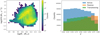 |
Fig. 1. Left: range of SFR and of M⋆ of the 15 765 535 sources in the WISExSCOS value-added catalogue in the range 0.1 < z < 0.3. Right: distributions of the active, transitioning, and passive galaxies of the WISExSCOS value-added catalogue as a function of redshift. |
2.1.2. Distance to the main-sequence estimation
Similar to estimating the star-forming activity of galaxies by computing specific SFR, which illustrates the efficiency of a galaxy in forming stars, the distance to the main sequence on an SFR-M⋆ diagram informs us about the star formation activity. This quantity, noted d2ms, is estimated following Bonjean et al. (2019) and can be a useful property to segregate populations of galaxies. We thus split the 15,765,535 sources of the WISExSCOS catalogue, in the range 0.1 < z < 0.3, into active, transitioning, and passive galaxies using the d2ms criterion. We defined as active galaxies sources with d2ms < 0.4, as transitioning galaxies sources with 0.4 < d2ms < 1.25, and as passive galaxies sources with d2ms > 1.25. These cuts are defined by the intersections of three Gaussians, fitted on the distribution of the d2ms on a sample of spectroscopic SDSS galaxies, used to model the three populations of galaxies. After the splitting, the catalogue contains 7 249 961 active, 4 353 744 transitioning, and 4 161 830 passive galaxies. The distributions of the three populations of galaxies in redshifts are shown in the right panel of Fig. 1.
2.1.3. Galaxy density maps
Based on the WISExSCOS value-added catalogue and on its three sub-samples of galaxy types defined above, we constructed 3D galaxy density maps in the redshift range 0.1 < z < 0.3, using the positions of the sources and their redshift information. To do so, we reconstructed the density field with a Python implementation4 of the Delaunay Tesselation Field Estimator (DTFE; Schaap & van de Weygaert 2000). Based on 3072 3D density fields in patches of 3.7° ×3.7°, we generated 4 sets of 20 sets of HEALPIX full-sky maps (20 for the 20 bins in redshift): one for all galaxies and one for each of the three populations of galaxies. We set nside = 2048 to the HEALPIX maps so that the pixel resolution is 1.7′ and the binning in redshift was arbitrarily set to δz = 0.01. We checked that the choice of the binning does not affect the results. An example of a slice at z = 0.15 of the 3D passive galaxy density map (smoothed at 30’ for visualisation) is shown in Fig. 2. The large-scale distribution of the galaxies is seen, together with contaminations, i.e. the stripes due to the WISE scanning strategy, the mask of our galaxy and the Magellanic cloud, and the reddening from dust around our galaxy and the Magellanic cloud. High-density concentrations, which are galaxy clusters, are also shown. In addition to the four galaxy density maps, we constructed 3D maps of SFR and M⋆ for all galaxies and for the active, transitioning, and passive populations using the same approach. The maps are constructed by linearly interpolating the estimated SFR and M⋆ quantities at their 3D positions.
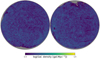 |
Fig. 2. Mollweide projection of the slice at z = 0.15 of the 3D passive galaxy density map constructed with the pyDTFE code. The map is smoothed at 30’ for visualisation. The large-scale distribution of the galaxies is shown, together with artefacts from the WISE scanning strategy, and the masks of our galaxy and of the Magellanic cloud. |
2.2. Catalogue of filaments
We used the SDSS Data Release 12 (DR12) LOWZCMASS spectroscopic sample of galaxies to construct a catalogue of cosmic filaments using DisPerSE (Sousbie 2011). The DisPerSE algorithm detects filaments in catalogues of discrete points. The method is based on the density field, reconstructed with the DTFE method. The DisPerSE method identifies critical points in the density field, i.e. points of maximum density, saddle points, bifurcation points, and points of minimum local density. This method then outputs a catalogue of filaments, constructed by connecting the saddle points to the maximum density points. Each filament is constituted by several segments, with given positions and redshifts. Also, DisPerSE outputs a persistence parameter for each filament. The persistence parameter is a topologically defined measurement of the significance of a given structure (e.g. a filament). This parameter is computed starting from the ratio of the DTFE densities of the critical points at the extrema of a filament. The persistence of a structure is usually expressed in the number of sigma it lies above the distribution of persistence values for a pure noise realisation in a manner similar to the definition of the signal-to-noise ratio. In the present case a threshold was set to 3σ. The details of the construction of the catalogue are given in Malavasi et al. (2020a,b). We defined the mean positions of the filaments (RAmean, Decmean) being the mean of the positions (RAi, Deci) of the i segments. In the following, we defined the minimum, mean, and maximum redshifts of the filaments, zmin, zmean, and zmax, as the minimum, mean, and maximum redshifts of the segments composing the filaments.
Since we are studying the properties of the WISExSCOS value-added catalogue, we thus excluded the filaments for which parts went outside the redshift range of the WISExSCOS catalogue, that is 0.1 < z < 0.3, to ensure that the filaments of our selection are entirely studied. We also cut the longest filaments at l > 100 Mpc, where l is the 3D length of the filament in Mpc, which may be unreliable filaments. We also excluded the filaments for which profiles were not complete so that each bin in profile has the same statistics. A final selection of n = 5559 cosmic filaments is used in our analysis. Their length and redshift distributions are shown in Fig. 3.
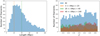 |
Fig. 3. Selection of the SDSS-DR12 LOWZCMASS DisPerSE filaments used. Left: three-dimensional length distribution. The orange dotted line shows the limit between the short and regular filaments, and the green dotted line shows the limit between the regular and long filaments. Right: redshift distribution of all filaments, overlaid with the redshift distributions of the filaments for the three bins of lengths. |
We split the 5559 selected DisPerSE filaments over three bins defined by their 3D length l (in Mpc) to later study the effect of the environment on galaxy properties around the filaments. In the following, we define “short”, “regular”, and “long” filaments, as follows:
-
3 < l < 20 : nobj = 1042,
-
20 < l < 40 : nobj = 2291,
-
40 < l < 100 : nobj = 2226.
For the case of short filaments, we set the upper limit to 20 Mpc based on the information given by the two-point correlation functions of groups in the 2DF survey (Yang et al. 2005), which infer that filaments below this typical size may be the tiniest and densest filaments, i.e. bridges of matter connecting two clusters, such as the bridge between A399 and A401 (Bonjean et al. 2018). We set the limit between the regular and long filaments arbitrarily to 40 Mpc to keep the same statistics in the two categories (about 2250 filaments in each). We checked that the choice of the binning in length does not affect the results. We also checked that the binning in length does not produce a bias of selection in redshift, as shown in the right panel of Fig. 3.
2.3. Galaxy cluster catalogues
We masked the over-density maps at the position of known clusters, preventing us from including galaxy cluster members while we computed the galaxy over-density profiles around the filaments. We used a combination of catalogues of galaxy cluster detected in X-ray, optical, and via the SZ effect for the masking. We masked 1478 clusters from the 2015 Planck PSZ2 clusters catalogue (Planck Collaboration XIII 2016), 1601 clusters from the MCXC5 ROSAT6 X-ray clusters catalogue (Piffaretti et al. 2011), 15 846 clusters from the galaxy clusters detected in optical in the Sloan Digital Sky Survey (SDSS, York et al. 2000) from RedMapper (Rykoff et al. 2014), 2395 from WHL 2015 (Wen & Han 2015), 75 045 from WHL 2012 (Wen et al. 2012), and 33,428 from AMF9 (Banerjee et al. 2018). We masked only galaxy clusters with z < 0.4 to ensure, in a conservative way, that most of the galaxy clusters in the redshift range 0.1 < z < 0.3 of the WISExSCOS catalogue are taken into account. In order to be very conservative, we also masked the catalogue of bifurcation points and of maximum density points with z < 0.4 provided by DisPerSE, as these points can be at positions of groups or clusters of galaxies that may not be detected in the galaxy cluster catalogues. We investigated the use of different masks in Sect. 3.2, where different radii for masking clusters have been used.
3. Measuring the profiles
3.1. Methodology
In order to measure the radial profiles of galaxy quantities around filaments, we used the RadFil code developed by Zucker & Chen (2018). The RadFil code takes two maps as inputs: one of the quantity of interest (the maps of galaxy densities constructed in Sect. 2.1) and one tracing the spine of the filament around which it performs the measurement (the maps tracing the spines of the selected DisPerSE filaments). Multiple steps were needed to obtain the radial profiles. These steps are described below.
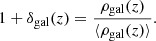
Step one is the normalisation of the maps. The galaxies in the WISExSCOS value-added catalogue are not uniformly distributed in redshift, and the three populations of galaxies do not follow the same distributions, as shown in Fig. 1. Thus, the values of the mean galaxy densities in each redshift slice of the galaxy density maps constructed in Sect. 2.1 also follow the same redshift distribution. Measuring the absolute value of the galaxy densities may thus introduce bias. To avoid this, and to measure only the excess of galaxies relative to the mean galaxy density in the field, we normalised the 3D density maps in order to consider over-densities δ. We divided each slice of redshift of each 3D map by their mean galaxy density values
 (1)
(1)
In that way, the 3D maps are transformed from biased densities ρgal to unbiased over-densities 1 + δgal.
Step two is the projection on patches. For each of the 5559 filaments, we projected the 3D maps of the obtained galaxy over-density 1 + δgal, on 3D patches centred on the position of the corresponding filament using a tangential projection. The 3D patches have a pixel resolution of θpix = 1.7 arcmin, a bin in redshift of 0.01 (same as the full-sky maps), and a number of pixels which depends on the length of the filament (computed in arcmin with the mean redshift zmean). Doing so, all filaments are entirely seen in their corresponding individual patch and the field of view of the largest patch is 19° ×19°. As 95% of the patches have fields of view below 15° ×15°, we neglected the projection effects and assumed the flat sky approximation.
Step three is the stack along the redshift axis. Because of the high value of the statistical error on the photometric redshifts of the sources in the WISExSCOS catalogue, σz = 0.033, 3D density profiles around filaments would be biased. Therefore, we stacked the 3D patches (obtained above) along the redshift axis to remove the uncertainty on the positions of the galaxies in the redshift space. The resulting stacked maps are thus 2D arrays. Before stacking along redshift, in order to minimise the noise due to background and foreground galaxies, we removed for each filament the regions of the 3D patch that lie outside the redshift range zmin − σz < z < zmax + σz, where zmin and zmax are the minimum and maximum redshifts of the filament. Mathematically, this step translates into
 (2)
(2)
where bz is the number of redshift bins in the range [zmin − σz, zmax + σz].
Step four is the application of RadFil. We applied RadFil with the 5559 2D stacked maps obtained above, together with the 5559 associated 2D spine projections of the filament, in the format of 2D arrays as well. RadFil then measures the radial profiles ⟨1 + δgal⟩(r) around each of the 5559 filaments.
Step five is the stack of the profiles. Finally, we stacked the 5559 profiles to get one unique profile, exhibiting statistical trends thanks to the significant reduction of the noise.
Final step is the estimation of the error bars. To estimate the error bars on the stacked profiles, we used the bootstrap method that resamples to ensure the significance of the detection. For the n measured profiles, where n is the number of filaments, we randomly selected n over n profiles with replacement and computed the mean profile. We repeated this measurement 1000 times and computed the mean and standard deviation of the 1000 mean profiles. The mean and standard deviations are taken as final measurements and errors in this study.
3.2. Masking the galaxy cluster members
In order to measure galaxy over-density profiles along filaments uncontaminated by the galaxy cluster members, we removed the regions around known galaxy clusters, by masking the maps at the position of the clusters presented in Sect. 2.3.
To mask the clusters in an optimal way, we defined six masks: the first one in which the galaxy clusters are not masked, and the five others in which the clusters were masked in regions from 1 × R500 to 5 × R500. The results are shown in Fig. A.1. The galaxy over-density profiles decrease with increasing radius of the mask, up to r = 3 × R500. Beyond this radius, the profiles are unchanged but the error bars increase. We thus chose to mask the clusters at r = 3 × R500. For clusters without estimated R500 (only a handful from the Planck catalogue in the SDSS area), we masked a region with radii increasing up to r = 10 arcmin. We show in Fig. A.2 that masking at r = 5 arcmin is enough, as no difference in the profiles is noticed. We also masked regions around the critical points provided by DisPerSE, namely the maxima density points, and the bifurcation points, with z < 0.4. For these regions, we masked regions with areas defined by radii varying up to r = 20 arcmin (see Fig. A.3). For the critical points, the profiles are decreasing with the increasing radii up to 20 arcmin. Part of the reason for the decrease of the profiles is caused by the loss of the shortest filaments in the selection (i.e. a change in the length distribution seen in the left panels). We chose to mask the critical points from DisPerSE at r = 10 arcmin, as it is a good compromise to keep the shortest filaments of about l < 7 Mpc in the selection of filaments while removing contamination from galaxies in small groups.
Finally, we also masked the area outside the footprint of the SDSS-DR12 area. The union mask is shown in orthographic projection in Fig. 4; only the northern hemisphere is shown, as none of the selected filaments are in the southern hemisphere.
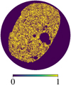 |
Fig. 4. Orthographic projection of the union mask of the northern hemisphere used in this analysis. |
3.3. Robustness of the measurement
To ensure the robustness of the measurements and compute their significance, we performed null tests. By applying the exact same methodology as that detailed above, we computed profiles in patches with the same properties as those of the 5559 DisPerSE filaments (number of pixels θpix and redshift range zmin − σz < z < zmax + σz), but centred on random positions on the sky and with random rotations. For computational time reasons, we computed only 100 random position stacked profiles. The null test was found compatible with zero at 1σ and has an offset of the order of 1%. However, this offset is negligible and does not change the interpretation of the observed galaxy over-density profiles around filaments, which were all detected with high significances, ranging between ∼5σ and 32σ. After testing for the effects of the DTFE, the interpolation on the HEALPIX pixels, and the redshift bins, we found that the offset is due to a combination of the mask and the spatial distribution of galaxies. Indeed, we verified that when we reshuffled the pixels in the footprint, the null test converged to the expected mean value of the map.
Although the profiles are very significantly detected, there are some effects that may produce biases and trends that may not be explicitly related to galaxies around filaments. We discuss the possible sources of contamination hereafter.
One of the main issues is the error on the photometric redshifts of the sources in the WISExSCOS catalogue, σz = 0.033. This error may induce a bias during the construction of the 3D density maps presented in Sect. 2.1 and make them not reliable in the redshift direction. To mitigate this effect, we computed the profiles in 2D projected maps stacked in the range [zmin − σz, zmax + σz], where zmin and zmax are the minimum and maximum redshifts of the filaments.
Another possible source of bias may be the 3D to 2D projection of the over-densities. The RadFil code computes profiles on 2D, while the filaments are defined as 3D structures. This may induce a bias in the shape of the profiles, especially when the axis of the filaments are not orthogonal to the line of sight. A comparison with numerical simulation should be done.
Another issue is the reliability of the filaments detected with DisPerSE. Indeed, although the LOWZCMASS sample was chosen to minimise these effects, the SDSS galaxies used for the detection may still suffer from, for example holes in the spatial distribution due to foreground bright stars or biased distribution in redshift due to magnitude limit selection. The position of the filaments and redshifts may also be affected by the noise of the survey, and by the finger-of-god effect of the galaxies in clusters (e.g. Jackson 1972), producing shifts of the galaxies in redshift space. The strategy adopted in this study to estimate over-density profiles of galaxies on a catalogue of galaxies (WISExSCOS) independent of that used to detect the filaments (SDSS) should reduce these biases, since the noises and biases of the two galaxy catalogues are independent. Moreover, we performed the exact same analysis around filaments detected with T-ReX, a regularised graph-based method (Bonnaire et al. 2020), and we find that the conclusions of this paper regarding the extension size of filaments and the properties of galaxies (star-forming, passive, sfr, mstar) are not altered.
4. Properties around cosmic filaments
4.1. Average properties
The stacked profile ⟨1 + δgal⟩ of the 5559 filaments selected from the DisPerSE catalogue is shown in blue in Fig. 5. The red lines and errors show the results of 100 null tests measurements on random positions and rotations. The binning in distance to the filament of the profiles is from r = 0.25 to r = 50 Mpc. We note that because of the pixel resolution of the galaxy density maps θpix, no information with a distance r < 0.25 Mpc is available. Profiles presented in this study thus show the behaviour of galaxies at large distances from the spines of the filament. We modelled the galaxy over-density profile by an exponential law (show in orange in Fig. 5), which takes the form
 (3)
(3)
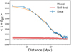 |
Fig. 5. In blue, the stacked radial profile of over-density ⟨1 + δgal⟩ of the galaxies from WISExSCOS catalogue around the 5559 filaments. In orange, the best-fit exponential model presented in Eq. (3). In red, 100 measurements on random positions from the null tests. |
where δgal0 is the mean projected over-density in the spines, rm the typical radius, and cgal is the offset discussed in Sect. 3.3. This offset is related to the interplay of the mask shape and the underlying galaxy distribution, which depends on the size of the filaments (shown later in Fig. 5). The fit of the model to the data with a least-squares minimisation gives δgal0 = 0.121 ± 0.002, rm = 7.5 ± 0.2 Mpc, and a very small offset cgal = 0.0093 ± 0.0004.
Although some studies have found that dark matter halo density profiles around filaments follow a power law with an index between −2 and −3 beyond 3 Mpc (Colberg et al. 2005; Dolag et al. 2006; Aragón-Calvo et al. 2010), the density profiles of galaxies around filaments have not been studied much. As shown in Cautun et al. (2014) and in Galárraga-Espinosa et al. (2020), filaments can be different in terms of width (with the largest widths from 2 Mpc to 10 Mpc), making the average density profiles of galaxies very dependent on the selection of filaments. In addition, the profiles presented in this work may also contain the correlations between the filaments, that is the probability to cross another filament up to a certain radius, and the probability to cross the same filament another time at another radius if the filament is curved. These effects would result in an enlargement of the profile. Hence, the value of the fitted typical radius rm = 7.5 ± 0.2 Mpc might be slightly overestimated.
To study the effect of the global environment, we averaged the galaxy over-density profiles in the three categories of filaments: the short, regular, and long filaments. The resulting profiles are shown in the left panel of Fig. 6. A small offset is seen for the regular filaments (cgal = 0.013) and the short filaments (cgal = 0.018). However, all three average profiles share the same shape. This trend is confirmed by the computation of the residuals of the three profiles with the exponential model (Eq. (3)) with the parameters from the average profile (δgal0 = 0.121 ± 0.002 and rm = 7.5 ± 0.2 Mpc). The residuals are shown in the right panel of Fig. 6. They do not show significant bias outside the error bars, suggesting that the galaxies around the small, regular, and long filaments share the same shapes or that the errors are too large to see a significant difference.
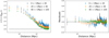 |
Fig. 6. Left: radial profiles of galaxy over-densities ⟨1 + δgal⟩ around cosmic filaments for short, regular, and long filaments. Right: residuals after substracting the exponential model fitted to the average over-density profile, shown in orange in Fig. 5, and the tiny offsets. |
We also computed the stacked profiles of excess of SFR and excess of M⋆, defined as ⟨1 + δSFR⟩ and ⟨1 + δM⋆⟩ in the same way as for ⟨1 + δgal⟩. The resulting stacked profiles for the short, regular, and long filaments are shown in Fig. 7. Gradients of SFR and M⋆ pointing towards the spines of the filaments are detected with a significance of 6.5σ and 9.5σ, respectively. Galaxies are significantly ∼10% more massive and ∼10% less star forming. This trend is expected since the excess of passive galaxies near the filament spines was already shown in several studies (e.g. Malavasi et al. 2017; Laigle et al. 2018; Kraljic et al. 2018; Sarron et al. 2019). This implies a different ratio of passive to active galaxies with increasing distance to the spine of the filament, producing these gradients. The M⋆ gradient is 60% higher in the case of short filaments. This trend is also expected, as short filaments may represent bridges of matter, i.e. more mature structures lying in the densest environments of the cosmic web (e.g. Aragón-Calvo et al. 2010) or events resulting from cluster interactions. These environments already show evidence of hot diffuse gas potentially inducing quenching of galaxies. For example in the bridge of matter between A399 and A401, most of the galaxies between the two clusters were found to be passive (Bonjean et al. 2018). Therefore, it is hard to identify the origin of the observed gradients at this stage. They may reflect a change in the galaxy populations or a real stellar mass gradient of all types of galaxies around filaments.
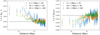 |
Fig. 7. Radial stacked profiles of excess of M⋆ and SFR: ⟨1 + δSFR⟩ and ⟨1 + δM⋆⟩ for the short, regular, and long filaments. |
4.2. Splitting over galaxy types
To explore further the impact of the environment on galaxy properties, we computed the stacked radial profiles on galaxies by splitting these profiles into three populations, i.e. active, transitioning, and passive. We used the 3D maps of galaxy densities constructed for the three types. The resulting stacked profiles ⟨1 + δgal⟩ around the short, regular, and long filaments are shown in Fig. 8.
 |
Fig. 8. Stacked radial over-density profiles of active (blue), transitioning (green), and passive (red) galaxies, as defined with the distance to the main sequence (detailed in Sect. 2.1.1) around the short, regular, and long cosmic filaments from left to right. |
The profiles of galaxy over-density decrease with galaxy types: the excess of passive galaxies around the spines of the filaments is higher than the excess of transitioning galaxies, and the excess of transitioning galaxies is higher than the excess of active galaxies. These results show that whatever the length of the filaments, more passive galaxies are distributed towards the spines of the filament. This indicates a quenching process inside the cosmic filaments, as already shown in for example Alpaslan et al. (2016), Martínez et al. (2016), Malavasi et al. (2017), Kraljic et al. (2018), Laigle et al. (2018) and Sarron et al. (2019). Another interesting trend to notice is the excess of passive galaxies, which is higher around short filaments than around regular and long filaments. This confirms the trend that short filaments may be bridges of matter. However, no difference is seen between regular and long filaments. These results show that from a length of 20 Mpc, cosmic filaments share on average the same properties and the same galaxy population distributions whatever their length.
We also computed the excess of M⋆ and SFR for the three galaxy types. The resulting stacked profiles are shown in Fig. 9. In the left panel, M⋆ gradient is shown for each type of galaxies, i.e. active, transitioning, and passive, detected at 2.2σ, 4.3σ, and 5.3σ, respectively. These results show that the galaxies are ∼5% more massive in the spine of the filaments, whatever the types. An M⋆ gradient towards the spines of the filaments in active galaxies was also detected in Malavasi et al. (2017) and Kraljic et al. (2018). This may be due to mergers of galaxies inside filaments (e.g. Codis et al. 2015; Malavasi et al. 2017). Our results are also in line with the results obtained by Alpaslan et al. (2016). These authors found a gradient of stellar mass in the direction of the spines of the filaments for spiral galaxies selected to belong to filaments. Our selection of active galaxies should indeed be similar to the selection of spiral galaxies in Alpaslan et al. (2016) since the latter tend to belong to the main sequence of galaxies. In the right panel of Fig. 9, a positive SFR gradient is detected at 6.3σ for passive galaxies alone. This suggests that passive galaxies are more star-forming inside the filaments. This trend could be due to the rejuvenation of the star formation in passive galaxies owing to gas accreted by galaxy mergers. For the population of active galaxies, no difference is seen in the SFR profile. This result is also in line with results by Alpaslan et al. (2016) who found an increasing specific SFR (sSFR) for spiral galaxies as a function of the distance to the spine of the filaments. Such an increase is obtained if the SFR profile of active galaxies is flat, which we find to be the case, and the stellar mass is decreasing, which we also find to be the case.
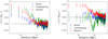 |
Fig. 9. Left: ⟨1 + δM⋆⟩ stacked radial profiles for each galaxy types: active galaxies in blue, transitioning galaxies in green, and passive galaxies in red. Right: ⟨1 + δSFR⟩ stacked radial profiles for the same galaxy types. |
5. Profile derived by the quenching
5.1. Quiescent fraction
The results of Sect. 4.2 indicate that galaxy populations are differently distributed towards the spines of the filaments, which motivated us to compute the fraction of quenched galaxies; this fraction is similar to the quiescent fraction fQ (e.g. Fontana et al. 2009; Hahn et al. 2015; Martis et al. 2016; Lian et al. 2016) but with galaxy over-densities rather than galaxy densities. In this case the quiescent fraction is defined as the ratio of the excess of passive galaxies ⟨1 + δgalP⟩ to the sum of the excess of passive ⟨1 + δgalP⟩ and active ⟨1 + δgalA⟩ galaxies as follows:
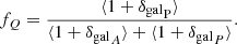 (4)
(4)
Since transitioning galaxies are in the process of quenching and can be defined both as star forming or quenched, we did not take these into account. The quiescent fraction fQ around cosmic filaments is shown in Fig. 10.
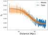 |
Fig. 10. In blue, the quiescent fraction profile fQ, averaged around the 5559 selected filaments. In orange, the β-model (Eq. (5)) from different realisations of the MCMC. |
5.2. Possible link to gas content
It is still not clear to date what are the dominant drivers of the quenching process in the galaxies. It has been already shown, and confirmed in the present study, that the cosmic web filaments have an impact on galaxy properties (e.g. Malavasi et al. 2017; Laigle et al. 2018; Kraljic et al. 2018; Sarron et al. 2019). Some studies have assumed the quenching is only due to the environment and the cosmic web via the hot gas in the haloes (T ≥ 105.4 K), thus preventing the galaxies from forming stars (Gabor & Davé 2015), or by cosmic web detachment (Aragon-Calvo et al. 2019). Peng et al. (2015) and Trussler et al. (2020) studied the effect of the gas of the cosmic web on the quenching of galaxies and conclude that starvation and strangulation were the main processes of quenching. In each of these studies, the quenching is thus related to the temperature or density of the gas, i.e. to the gas pressure around the cosmic web.
In Tanimura et al. (2020), we studied hot gas via the SZ emission around cosmic filaments detected with DisPerSE on SDSS galaxies in the range 0.2 < z < 0.6. The temperature of the gas around the filaments is estimated to be T ∼ 106 K (larger than the temperature of quenching of the haloes found in Gabor & Davé 2015: T ≥ 105.4 K).
The quiescent fraction profile measured in the previous section and shown in Fig. 10 might depend mostly on the processes of quenching, which drives the population changeover. We modelled in a simple way the fQ profile with a model of gas density distribution around the cosmic filaments. We used a β-model (historically used to model the gas density profiles in galaxy clusters; Cavaliere & Fusco-Femiano 1978). This model is written as
 (5)
(5)
where fQ0 is the mean ratio of excess of passive galaxies over the sum of the excess of active and passive galaxies in the centre of the filaments, rs is the core radius, β the slope of the profile, and c is the background value.
We performed a Markov chain Monte Carlo (MCMC) analysis and obtained the posterior distributions of the four parameters of Eq. (5). The distributions and correlations are shown in Fig. 11. Figure 10 also shows 1000 models randomly picked from the MCMC distribution. The median parameters are fQ0 = 0.017 ± 0.003, rs = 4.4 ± 1.7 Mpc, β = 0.54 ± 0.18, and the background value c = 0.498 ± 0.001. Assuming the quiescent fraction of galaxies traces the pressure of the gas responsible for the quenching, the values of the slope β of the gas profile and the quiescent fraction profile should be the same. The slope β is not well constrained as seen in the distribution in Fig. 11: this parameter is fully degenerate with the parameter rs. However, β = 2/3, which is the case for projected iso-thermal gas in hydrostatic equilibrium (scenario supported by numerical simulation, e.g. in Gheller & Vazza 2019), is encompassed in the values allowed by the MCMC. Moreover, the value β = 2/3 that fits the gas profile in SZ in Tanimura et al. (2020) is also encompassed in the allowed values by the MCMC.
 |
Fig. 11. Posterior distributions of the four parameters of the β-model (Eq. (5)) fitted to the quiescent fraction profile shown in Fig. 10. |
6. Discussion and summary
We have studied in detail the statistical properties of the galaxies from the WISExSCOS value-added catalogue around cosmic filaments detected with DisPerSE in the SDSS. We measured with a high significance (≳5σ) galaxy over-density radial profiles on the full sample of galaxies and also on the three populations: i.e. active, transitioning, and passive galaxies.
Despite some biases on the measurement due to the methodology or to the data themselves, we fitted an average profile of galaxy over-density around cosmic filaments with an exponential law. We obtained a typical radius of rm = 7.5 ± 0.2 Mpc. We also pointed out the evidence of a higher excess of passive galaxies than transitioning galaxies, and a higher excess of transitioning galaxies than active galaxies near the filament spines. This excess of passive galaxies induces an SFR and an M⋆ gradient pointing towards the filament spines, which we also detected. This indicates that there are more passive galaxies near the filament spines, in agreement with the previous studies (e.g. Malavasi et al. 2017; Kraljic et al. 2018; Laigle et al. 2018; Sarron et al. 2019).
We also studied the excess of M⋆ and of SFR for the three galaxy populations and pointed out the evidence of a positive M⋆ gradient for active, transitioning, and passive populations of galaxies. This means that galaxies are more massive in the filaments, whatever their types, in agreement with Alpaslan et al. (2016), Kraljic et al. (2018), and Malavasi et al. (2017) who observed a stellar mass gradient for spiral or star-forming galaxies. We also detected a positive SFR gradient for passive galaxies, showing that passive galaxies are more star forming in the filaments. These gradients could be related to galaxy merges inside filaments, which increase the M⋆ of the galaxies and may rejuvenate the SFR in passive galaxies. We did not find any change in SFR for active galaxies, in agreement with results from Alpaslan et al. (2016) who found an increasing sSFR as a function to the distance of the spines of the filaments, which can be explained by our observation of decrease in stellar mass and no change in SFR.
We investigated how the quiescent fraction of galaxies, fQ, behaves around cosmic filaments. Following previous studies showing the role of the cosmic web and of the gas in the quenching of star formation, and following the recent detection of diffuse hot gas around cosmic filaments in SZ with T ∼ 106 K, we modelled in an exploratory way the fQ profile with a model of gas density distribution. We measured parameters with an MCMC analysis. The obtained slope β = 0.54 ± 0.18 is not well constrained. However, the MCMC distribution encompasses the value β = 2/3, which is the case for projected iso-thermal gas in hydrostatic equilibirum suggested for example by Gheller & Vazza (2019). The MCMC distribution of β also encompasses the values of β fitted on gas profile with SZ. The slope of the quiescent fraction profile is not inconsistent with the slope of a gas profile around cosmic filaments. Therefore, in this exploratory work, it is not excluded that the gas around cosmic filaments might have a non-negligible role in the quenching of star formation in galaxies.
To capture and understand the connections between the cosmic web environment and galaxy properties, the profiles derived and shown in this study will be compared with numerical simulations in Illustris-TNG (Galárraga-Espinosa et al. 2020) and with observations of the gas around cosmic filaments (with the SZ effect in Planck or in the X-rays with the future e-Rosita7 mission). In the context of future very large galaxy surveys like Euclid8, LSST9, or WFIRST10, such studies on galaxy properties will be possible for a broader range of redshift, for a wider field of view, and thus with a higher significance.
Discrete Persistent Structure Extractor.
Tree-based Ridge eXtractor.
Meta-Catalogue of X-ray Clusters.
Röntgensatellit.
Acknowledgments
The authors thank the anonymous referee for her/his useful comments. The authors also thank useful discussions with Dr. Guillaume Hurier, and with all the members of the ByoPiC project (https://byopic.eu/team). This research has been supported by the funding for the ByoPiC project from the European Research Council (ERC) under the European Union’s Horizon 2020 research and innovation programme grant agreement ERC-2015-AdG 695561. This publication made use of the SZ-Cluster Database (http://szcluster-db.ias.u-psud.fr) operated by the Integrated Data and Operation Centre (IDOC) at the Institut d’Astrophysique Spatiale (IAS) under contract with CNES and CNRS. This research has made use of data obtained from the SuperCOSMOS Science Archive, prepared and hosted by the Wide Field Astronomy Unit, Institute for Astronomy, University of Edinburgh, funded by the UK Science and Technology Facilities Council.
References
- Adhikari, S., Dalal, N., More, S., & Wetzel, A. 2019, ApJ, 878, 9 [Google Scholar]
- Akamatsu, H., Fujita, Y., Akahori, T., et al. 2017, A&A, 606, A1 [NASA ADS] [CrossRef] [EDP Sciences] [Google Scholar]
- Alpaslan, M., Driver, S., Robotham, A. S. G., et al. 2015, MNRAS, 451, 3249 [NASA ADS] [CrossRef] [Google Scholar]
- Alpaslan, M., Grootes, M., Marcum, P. M., et al. 2016, MNRAS, 457, 2287 [NASA ADS] [CrossRef] [Google Scholar]
- Aragón-Calvo, M. A., van de Weygaert, R., & Jones, B. J. T. 2010, MNRAS, 408, 2163 [NASA ADS] [CrossRef] [Google Scholar]
- Aragon-Calvo, M. A., Neyrinck, M. C., & Silk, J. 2019, Open J. Astrophys., 2, 7 [CrossRef] [Google Scholar]
- Arnaud, M., Pratt, G. W., Piffaretti, R., et al. 2010, A&A, 517, A92 [NASA ADS] [CrossRef] [EDP Sciences] [Google Scholar]
- Banerjee, P., Szabo, T., Pierpaoli, E., et al. 2018, New Astron., 58, 61 [NASA ADS] [CrossRef] [Google Scholar]
- Bartalucci, I., Arnaud, M., Pratt, G. W., et al. 2017, A&A, 608, A88 [NASA ADS] [CrossRef] [EDP Sciences] [Google Scholar]
- Baxter, E., Chang, C., Jain, B., et al. 2017, ApJ, 841, 18 [NASA ADS] [CrossRef] [Google Scholar]
- Bilicki, M., Peacock, J. A., Jarrett, T. H., et al. 2016, ApJS, 225, 5 [NASA ADS] [CrossRef] [Google Scholar]
- Bond, J. R., Kofman, L., & Pogosyan, D. 1996, Nature, 380, 603 [NASA ADS] [CrossRef] [Google Scholar]
- Bonjean, V., Aghanim, N., Salomé, P., Douspis, M., & Beelen, A. 2018, A&A, 609, A49 [NASA ADS] [CrossRef] [EDP Sciences] [Google Scholar]
- Bonjean, V., Aghanim, N., Salomé, P., et al. 2019, A&A, 622, A137 [NASA ADS] [CrossRef] [EDP Sciences] [Google Scholar]
- Bonnaire, T., Aghanim, N., Decelle, A., & Douspis, M. 2020, A&A, 637, A18 [NASA ADS] [CrossRef] [EDP Sciences] [Google Scholar]
- Bykov, A. M., Churazov, E. M., Ferrari, C., et al. 2015, SSR, 188, 141 [NASA ADS] [Google Scholar]
- Cautun, M., van de Weygaert, R., & Jones, B. J. T. 2013, MNRAS, 429, 1286 [NASA ADS] [CrossRef] [Google Scholar]
- Cautun, M., van de Weygaert, R., Jones, B. J. T., & Frenk, C. S. 2014, MNRAS, 441, 2923 [NASA ADS] [CrossRef] [Google Scholar]
- Cavaliere, A., & Fusco-Femiano, R. 1978, A&A, 70, 677 [NASA ADS] [Google Scholar]
- Chang, C., Baxter, E., Jain, B., et al. 2018, ApJ, 864, 83 [CrossRef] [Google Scholar]
- Chen, Y.-C., Ho, S., Mandelbaum, R., et al. 2017, MNRAS, 466, 1880 [NASA ADS] [CrossRef] [Google Scholar]
- Codis, S., Pichon, C., & Pogosyan, D. 2015, MNRAS, 452, 3369 [Google Scholar]
- Colberg, J. M., Krughoff, K. S., & Connolly, A. J. 2005, MNRAS, 359, 272 [NASA ADS] [CrossRef] [Google Scholar]
- de Graaff, A., Cai, Y.-C., Heymans, C., & Peacock, J. A. 2019, A&A, 624, A48 [NASA ADS] [CrossRef] [EDP Sciences] [Google Scholar]
- Dolag, K., Meneghetti, M., Moscardini, L., Rasia, E., & Bonaldi, A. 2006, MNRAS, 370, 656 [NASA ADS] [Google Scholar]
- Dubois, Y., Pichon, C., Welker, C., et al. 2014, MNRAS, 444, 1453 [NASA ADS] [CrossRef] [Google Scholar]
- Eckert, D., Jauzac, M., Shan, H., et al. 2015, Nature, 528, 105 [NASA ADS] [CrossRef] [Google Scholar]
- Fontana, A., Santini, P., Grazian, A., et al. 2009, A&A, 501, 15 [NASA ADS] [CrossRef] [EDP Sciences] [Google Scholar]
- Fujita, Y., Koyama, K., Tsuru, T., & Matsumoto, H. 1996, PASJ, 48, 191 [NASA ADS] [Google Scholar]
- Fujita, Y., Tawa, N., Hayashida, K., et al. 2008, PASJ, 60, S343 [NASA ADS] [CrossRef] [Google Scholar]
- Gabor, J. M., & Davé, R. 2015, MNRAS, 447, 374 [NASA ADS] [CrossRef] [Google Scholar]
- Galárraga-Espinosa, D., Aghanim, N., Langer, M., Gouin, C., & Malavasi, N. 2020, A&A, submitted [arXiv:2003.09697] [Google Scholar]
- Gheller, C., & Vazza, F. 2019, MNRAS, 486, 981 [NASA ADS] [CrossRef] [Google Scholar]
- Gheller, C., Vazza, F., Favre, J., & Brüggen, M. 2015, MNRAS, 453, 1164 [Google Scholar]
- Gheller, C., Vazza, F., Brüggen, M., et al. 2016, MNRAS, 462, 448 [NASA ADS] [CrossRef] [Google Scholar]
- Ghirardini, V., Eckert, D., Ettori, S., et al. 2019, A&A, 621, A41 [NASA ADS] [CrossRef] [EDP Sciences] [Google Scholar]
- Gouin, C., Aghanim, N., Bonjean, V., & Douspis, M. 2020, A&A, 635, A195 [NASA ADS] [CrossRef] [EDP Sciences] [Google Scholar]
- Hahn, C., Blanton, M. R., Moustakas, J., et al. 2015, ApJ, 806, 162 [NASA ADS] [CrossRef] [Google Scholar]
- Hirschmann, M., Dolag, K., Saro, A., et al. 2014, MNRAS, 442, 2304 [NASA ADS] [CrossRef] [Google Scholar]
- Jackson, J. C. 1972, MNRAS, 156, 1P [Google Scholar]
- Kraljic, K., Arnouts, S., Pichon, C., et al. 2018, MNRAS, 474, 547 [NASA ADS] [CrossRef] [EDP Sciences] [Google Scholar]
- Kravtsov, A. V., & Borgani, S. 2012, ARA&A, 50, 353 [NASA ADS] [CrossRef] [Google Scholar]
- Kuutma, T., Tamm, A., & Tempel, E. 2017, A&A, 600, L6 [NASA ADS] [CrossRef] [EDP Sciences] [Google Scholar]
- Laigle, C., Pichon, C., Arnouts, S., et al. 2018, MNRAS, 474, 5437 [NASA ADS] [CrossRef] [Google Scholar]
- Lian, J., Yan, R., Zhang, K., & Kong, X. 2016, ApJ, 832, 29 [Google Scholar]
- Libeskind, N. I., van de Weygaert, R., Cautun, M., et al. 2018, MNRAS, 473, 1195 [NASA ADS] [CrossRef] [Google Scholar]
- Mahajan, S., & Raychaudhury, S. 2009, MNRAS, 400, 687 [NASA ADS] [CrossRef] [Google Scholar]
- Mahajan, S., Mamon, G. A., & Raychaudhury, S. 2011, MNRAS, 416, 2882 [NASA ADS] [CrossRef] [Google Scholar]
- Malavasi, N., Arnouts, S., Vibert, D., et al. 2017, MNRAS, 465, 3817 [NASA ADS] [CrossRef] [EDP Sciences] [Google Scholar]
- Malavasi, N., Aghanim, N., Douspis, M., Tanimura, H., & Bonjean, V. 2020a, A&A, submitted [arXiv:2002.01486] [Google Scholar]
- Malavasi, N., Aghanim, N., Tanimura, H., Bonjean, V., & Douspis, M. 2020b, A&A, 634, A30 [NASA ADS] [CrossRef] [EDP Sciences] [Google Scholar]
- Martínez, H. J., Muriel, H., & Coenda, V. 2016, MNRAS, 455, 127 [NASA ADS] [CrossRef] [Google Scholar]
- Martis, N. S., Marchesini, D., Brammer, G. B., et al. 2016, ApJ, 827, L25 [CrossRef] [Google Scholar]
- Martizzi, D., Vogelsberger, M., Artale, M. C., et al. 2019, MNRAS, 486, 3766 [Google Scholar]
- Nagai, D., Vikhlinin, A., & Kravtsov, A. V. 2007, ApJ, 655, 98 [NASA ADS] [CrossRef] [Google Scholar]
- Peng, Y., Maiolino, R., & Cochrane, R. 2015, Nature, 521, 192 [NASA ADS] [CrossRef] [Google Scholar]
- Piffaretti, R., Arnaud, M., Pratt, G. W., Pointecouteau, E., & Melin, J.-B. 2011, A&A, 534, A109 [NASA ADS] [CrossRef] [EDP Sciences] [Google Scholar]
- Pintos-Castro, I., Yee, H. K. C., Muzzin, A., Old, L., & Wilson, G. 2019, ApJ, 876, 40 [Google Scholar]
- Planck Collaboration XIII. 2016, A&A, 594, A13 [NASA ADS] [CrossRef] [EDP Sciences] [Google Scholar]
- Planck Collaboration XXVII. 2016, A&A, 594, A27 [NASA ADS] [CrossRef] [EDP Sciences] [Google Scholar]
- Planck Collaboration Int. V. 2013, A&A, 550, A131 [NASA ADS] [CrossRef] [EDP Sciences] [Google Scholar]
- Planck Collaboration Int. VIII. 2013, A&A, 550, A134 [NASA ADS] [CrossRef] [EDP Sciences] [Google Scholar]
- Rykoff, E. S., Rozo, E., Busha, M. T., et al. 2014, ApJ, 785, 104 [NASA ADS] [CrossRef] [Google Scholar]
- Sakelliou, I., & Ponman, T. J. 2004, MNRAS, 351, 1439 [NASA ADS] [CrossRef] [Google Scholar]
- Sarron, F., Adami, C., Durret, F., & Laigle, C. 2019, A&A, 632, A49 [NASA ADS] [CrossRef] [EDP Sciences] [Google Scholar]
- Schaap, W. E., & van de Weygaert, R. 2000, A&A, 363, L29 [Google Scholar]
- Sousbie, T. 2011, MNRAS, 414, 350 [NASA ADS] [CrossRef] [Google Scholar]
- Springel, V. 2005, MNRAS, 364, 1105 [NASA ADS] [CrossRef] [Google Scholar]
- Springel, V., Pakmor, R., Pillepich, A., et al. 2018, MNRAS, 475, 676 [NASA ADS] [CrossRef] [Google Scholar]
- Sunyaev, R. A., & Zeldovich, Y. B. 1970, ApSS, 7, 20 [NASA ADS] [Google Scholar]
- Sunyaev, R. A., & Zeldovich, Y. B. 1972, Comments Astrophys. Space Phys., 4, 173 [NASA ADS] [EDP Sciences] [Google Scholar]
- Tanimura, H., Aghanim, N., Douspis, M., Beelen, A., & Bonjean, V. 2019a, A&A, 625, A67 [NASA ADS] [CrossRef] [EDP Sciences] [Google Scholar]
- Tanimura, H., Hinshaw, G., McCarthy, I. G., et al. 2019b, MNRAS, 483, 223 [NASA ADS] [CrossRef] [Google Scholar]
- Tanimura, H., Aghanim, N., Bonjean, V., Malavasi, N., & Douspis, M. 2020, A&A, 637, A41 [CrossRef] [EDP Sciences] [Google Scholar]
- Tempel, E., Stoica, R. S., Kipper, R., & Saar, E. 2016, Astron. Comput., 16, 17 [NASA ADS] [CrossRef] [Google Scholar]
- Trussler, J., Maiolino, R., Maraston, C., et al. 2020, MNRAS, 491, 5406 [CrossRef] [Google Scholar]
- Walker, S., Simionescu, A., Nagai, D., et al. 2019, SSR, 215, 7 [NASA ADS] [Google Scholar]
- Wen, Z. L., & Han, J. L. 2015, ApJ, 807, 178 [NASA ADS] [CrossRef] [Google Scholar]
- Wen, Z. L., Han, J. L., & Liu, F. S. 2012, ApJS, 199, 34 [NASA ADS] [CrossRef] [Google Scholar]
- Yang, X., Mo, H. J., van den Bosch, F. C., & Jing, Y. P. 2005, MNRAS, 357, 608 [NASA ADS] [CrossRef] [Google Scholar]
- York, D. G., Adelman, J., Anderson, J. E., Jr, et al. 2000, AJ, 120, 1579 [CrossRef] [Google Scholar]
- Zel’Dovich, Y. B. 1970, A&A, 500, 13 [Google Scholar]
- Zucker, C., & Chen, H. H.-H. 2018, ApJ, 864, 152 [NASA ADS] [CrossRef] [EDP Sciences] [Google Scholar]
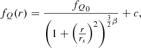
Appendix A: Masking the galaxy cluster members
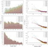 |
Fig. A.1. Comparison of the effect of different masks. Galaxy clusters with z < 0.4 from the PSZ2, MCXC, RedMaPPer, AMF9, WHL12, and WHL15 catalogues are masked with areas of radii from 0 to 5 × R500. Left and right columns: histogram of the filament lengths and over-density profiles ⟨1 + δgal⟩, respectively, for short, regular, and long filaments (from top to bottom). We chose the mask at 3 × R500. |
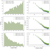 |
Fig. A.2. Comparison of the effect of different masks. For the galaxy clusters without estimated radius in the Planck PSZ2 catalogue with z < 0.4, regions defined by areas of 0, 5, and 10 arcmin radii are masked. No difference is noticed and all plots are overlapping. To clearly see the different profiles, we added +0.1 and +0.2 to the y-axis for the orange line and the green line, respectively. We therefore chose to mask at 5 arcmin. |
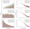 |
Fig. A.3. Comparison of the effect of different masks. Two types of critical points given by DisPerSE are masked: the maxima density points and the bifurcation points. The regions around the critical points with z < 0.4 are masked from 0 to 20 arcmin. Right panel: the signal is decreasing with the size of the masks for short and regular filaments. Left panel: the masks remove the short filaments. |
All Figures
|
Fig. 1. Left: range of SFR and of M⋆ of the 15 765 535 sources in the WISExSCOS value-added catalogue in the range 0.1 < z < 0.3. Right: distributions of the active, transitioning, and passive galaxies of the WISExSCOS value-added catalogue as a function of redshift. |
| In the text | |
|
Fig. 2. Mollweide projection of the slice at z = 0.15 of the 3D passive galaxy density map constructed with the pyDTFE code. The map is smoothed at 30’ for visualisation. The large-scale distribution of the galaxies is shown, together with artefacts from the WISE scanning strategy, and the masks of our galaxy and of the Magellanic cloud. |
| In the text | |
|
Fig. 3. Selection of the SDSS-DR12 LOWZCMASS DisPerSE filaments used. Left: three-dimensional length distribution. The orange dotted line shows the limit between the short and regular filaments, and the green dotted line shows the limit between the regular and long filaments. Right: redshift distribution of all filaments, overlaid with the redshift distributions of the filaments for the three bins of lengths. |
| In the text | |
|
Fig. 4. Orthographic projection of the union mask of the northern hemisphere used in this analysis. |
| In the text | |
|
Fig. 5. In blue, the stacked radial profile of over-density ⟨1 + δgal⟩ of the galaxies from WISExSCOS catalogue around the 5559 filaments. In orange, the best-fit exponential model presented in Eq. (3). In red, 100 measurements on random positions from the null tests. |
| In the text | |
|
Fig. 6. Left: radial profiles of galaxy over-densities ⟨1 + δgal⟩ around cosmic filaments for short, regular, and long filaments. Right: residuals after substracting the exponential model fitted to the average over-density profile, shown in orange in Fig. 5, and the tiny offsets. |
| In the text | |
|
Fig. 7. Radial stacked profiles of excess of M⋆ and SFR: ⟨1 + δSFR⟩ and ⟨1 + δM⋆⟩ for the short, regular, and long filaments. |
| In the text | |
|
Fig. 8. Stacked radial over-density profiles of active (blue), transitioning (green), and passive (red) galaxies, as defined with the distance to the main sequence (detailed in Sect. 2.1.1) around the short, regular, and long cosmic filaments from left to right. |
| In the text | |
|
Fig. 9. Left: ⟨1 + δM⋆⟩ stacked radial profiles for each galaxy types: active galaxies in blue, transitioning galaxies in green, and passive galaxies in red. Right: ⟨1 + δSFR⟩ stacked radial profiles for the same galaxy types. |
| In the text | |
|
Fig. 10. In blue, the quiescent fraction profile fQ, averaged around the 5559 selected filaments. In orange, the β-model (Eq. (5)) from different realisations of the MCMC. |
| In the text | |
|
Fig. 11. Posterior distributions of the four parameters of the β-model (Eq. (5)) fitted to the quiescent fraction profile shown in Fig. 10. |
| In the text | |
|
Fig. A.1. Comparison of the effect of different masks. Galaxy clusters with z < 0.4 from the PSZ2, MCXC, RedMaPPer, AMF9, WHL12, and WHL15 catalogues are masked with areas of radii from 0 to 5 × R500. Left and right columns: histogram of the filament lengths and over-density profiles ⟨1 + δgal⟩, respectively, for short, regular, and long filaments (from top to bottom). We chose the mask at 3 × R500. |
| In the text | |
|
Fig. A.2. Comparison of the effect of different masks. For the galaxy clusters without estimated radius in the Planck PSZ2 catalogue with z < 0.4, regions defined by areas of 0, 5, and 10 arcmin radii are masked. No difference is noticed and all plots are overlapping. To clearly see the different profiles, we added +0.1 and +0.2 to the y-axis for the orange line and the green line, respectively. We therefore chose to mask at 5 arcmin. |
| In the text | |
|
Fig. A.3. Comparison of the effect of different masks. Two types of critical points given by DisPerSE are masked: the maxima density points and the bifurcation points. The regions around the critical points with z < 0.4 are masked from 0 to 20 arcmin. Right panel: the signal is decreasing with the size of the masks for short and regular filaments. Left panel: the masks remove the short filaments. |
| In the text | |
Current usage metrics show cumulative count of Article Views (full-text article views including HTML views, PDF and ePub downloads, according to the available data) and Abstracts Views on Vision4Press platform.
Data correspond to usage on the plateform after 2015. The current usage metrics is available 48-96 hours after online publication and is updated daily on week days.
Initial download of the metrics may take a while.