© ESO 2020

1. Introduction

Gravitational lensing is a powerful tool in unveiling the true distribution of matter in the Universe and probing cosmological parameters (see, e.g. Kilbinger 2015 for a recent review). The lensing signal is sensitive to all matter, regardless of its nature, and is observed as the distortion of light bundles travelling through the Universe. In the weak lensing regime, this distortion is small and must be studied with large statistical samples. Therefore, large and deep surveys are required, for example, the Kilo Degree Survey¹ (KiDS); the Dark Energy Survey² (DES); the Hyper Suprime-Cam Subaru Strategic Program³ (HSC SSP); or the near-future surveys with Euclid⁴ and the Large Synoptic Survey Telescope⁵ (LSST). To maximise the scientific output from these surveys, the scientific community is currently putting great efforts into understanding nuances in the theoretical framework.

Galaxy-galaxy lensing (GGL) correlates the position of foreground galaxies to the distortion of background galaxies (see, e.g. Hoekstra 2013). The distortion is typically measured in terms of mean tangential shear with respect to the lens position. This shear signal, as a function of separation from the lens centre, can be related to the underlying mass properties of the parent halo. A major challenge is obtaining an unbiased mass estimate. Biases arise if the underlying model does not describe all contributions to the matter-shear correlation function sufficiently. Also, the galaxy bias that connects the position of galaxies to its surrounding matter distribution must be carefully taken into account. For current and future surveys, we must further consider second-order effects to the galaxy-matter correlation, such as, for example, magnification effects (Ziour & Hui 2008; Hilbert et al. 2009) and intrinsic alignment of galaxies (Troxel & Ishak 2015). In this work, we focus on the former effect.

Magnification is the change of the observed solid angle of an image compared to the intrinsic solid angle, or, since the surface brightness remains constant, the ratio of observed flux to the intrinsic one. Like the shear, it is a local quantity, a direct prediction of the lensing formalism, and is caused by all matter between the observed galaxy population and us. However, direct measurements of magnification are challenging because the intrinsic flux is typically unknown. Yet, the change in size and magnitude results in a changed spatial distribution of the galaxy population. This so-called number count magnification has been measured (e.g. Chiu et al. 2016; Garcia-Fernandez et al. 2018). Consequently, magnification by the large-scale structure (LSS) also changes the GGL signal compared to a signal that is just given by matter correlated with the lens galaxies. We stress that the magnification changes the number counts of the source as well as lens galaxies on the sky. The impact of magnification of the lens galaxies on the GGL signal for surveys like CFHTLenS is ∼5% (Simon & Hilbert 2018), but can be as large as 20% for other lens samples (Hilbert et al. 2009). Although these results suggest a fairly large impact of magnification on GGL lensing estimates, quantitative analyses widely neglect the influence of magnification. Unruh et al. (2019) studied the impact of the number count magnification of lens galaxies on the shear-ratio. They found that the shear-ratio test (Jain & Taylor 2003) is affected by lens magnification and that its effect must be mitigated, especially for high-lens redshifts.

In this paper, we quantify the impact of magnification on observed tangential shear profiles and halo-mass estimates from GGL. We consider both the effect of magnification of the sources by the lenses, as well as the effect of magnification of the lenses by the LSS. For this, we compared the GGL signal with and without magnification using simulated data. We then derived mean halo masses in both cases employing a halo model to quantify the expected mass bias. We complemented the numerical results with analytic estimates of the effects.

This article is organised as follows. The theoretical framework is briefly described in Sect. 2. Section 3 features an analytical description of how magnification affects shear estimates, as well as a brief discussion of how numerical results were obtained in this study. The numerical procedure is then more thoroughly explained in Appendix A. In Sect. 4, we discuss the impact of magnification of source galaxies by the lenses, and in Sect. 5 we discuss magnification of the lens galaxies by the LSS. We study the magnification bias on mass estimates in Sect. 6 and conclude in Sect. 7.

2. Theory

In the following, we introduce the theoretical concepts of gravitational lensing for this work. For a more general and extensive overview, the reader is kindly referred to Bartelmann & Schneider (2001).

2.1. Cosmological distances

For a flat universe, the Hubble parameter H(z) can be written as

$$\begin{array}{c}\hfill {\left(\frac{H(z)}{H_0}\right)}^2={\mathrm{\Omega }}_{\mathrm{m}}{(1+z)}^3+1-{\mathrm{\Omega }}_{\mathrm{m}},\end{array}$$(1)

where z is the redshift, H₀ denotes the Hubble constant, and Ω_m is the matter density in units of today’s critical density ${\rho }_{\text{crit}}=3H_0^2/(8\pi G)$; with the vacuum speed of light c and the gravitational constant G. The comoving distance travelled by a photon between redshift z₁ and z₂ reads

$$\begin{array}{c}\hfill \chi (z_1,z_2)={\displaystyle {\int }_{z_1}^{z_2}\frac{c\mathrm{d}{z}^{\prime }}{H(z^{\prime })},}\end{array}$$(2)

and the angular-diameter distance is

$$\begin{array}{c}\hfill D(z_1,z_2)=\frac{\chi (z_1,z_2)}{1+z_2}·\end{array}$$(3)

For a redshift z₁ = 0, which is the observer’s position, we write D(0, z) = : D(z). In addition, the dimensionless Hubble parameter h is used to parametrise our ignorance about the true value of today’s Hubble parameter, defined as H₀ = 100 h km s⁻¹ Mpc⁻¹. In the following, all distances are angular-diameter distances.

2.2. Gravitational lensing distortions and magnification

Gravitational lensing distorts the appearance of galaxy images. In the weak lensing regime, this distortion can locally be described as a linear mapping from the background (source) plane to the foreground (lens) plane. The Jacobian 𝒜 of the local mapping can be written as

$$\begin{array}{cc}\hfill \mathcal{A}& =\left(\begin{array}{cc}1-\kappa -{\gamma }_1& -{\gamma }_2\\ -{\gamma }_2& 1-\kappa +{\gamma }_1\end{array}\right)=(1-\kappa )\left(\begin{array}{cc}1-g_1& -g_2\\ -g_2& 1+g_1\end{array}\right),\hfill \end{array}$$(4)

where κ is the convergence, γ_1, 2 are the two Cartesian shear components, and g_1, 2 = γ_1, 2/(1 − κ) are the two Cartesian reduced shear components, which all depend on the position in the lens plane. The convergence causes an isotropic scaling of the galaxy image, while the shear leads to an anisotropic stretching, and thus causes an initially circular object to appear elliptical.

This scaling of the galaxy image changes the apparent solid angle ω of the image, compared to one in the absence of lensing, which we denote by ω₀. Likewise, the flux is affected by gravitational lensing, the unlensed flux s₀ is enhanced or reduced to the observed flux s. The ratio of these quantities defines the magnification μ and can also be calculated from the Jacobian by

$$\begin{array}{c}\hfill \mu =\frac{\omega }{{\omega }_0}=\frac{s}{s_0}=\frac{1}{det\mathcal{A}}=\frac{1}{{(1-\kappa )}^2-{|\gamma |}^2}·\end{array}$$(5)

Magnification changes the observed local number density of galaxies on the sky. The cumulative observed number density of galaxies on the sky n(> s), brighter than flux s, is locally

$$\begin{array}{c}\hfill n(>s)=\frac{1}{\mu }{n}_0(>\frac{s}{\mu }),\end{array}$$(6)

where n₀ denotes the cumulative number density in absence of lensing. The prefactor 1/μ is due to the scaling of the solid angle. The flux in the argument of n₀ must also be scaled by 1/μ to account for the flux enhancement or reduction.

Magnification effects in the weak lensing limit are small, specifically |μ − 1| ≪ 1, and we Taylor expand Eq. (6) in (μ − 1) to obtain to first order

$$\begin{array}{c}\hfill \frac{n(>s)}{n_0(>s)}={\mu }^{\alpha -1},\end{array}$$(7)

where the exponent α is the local slope at the flux limit s_lim, it is defined as

$$\begin{array}{c}\hfill \alpha =-\frac{\mathrm{d}{log}_{10}{n}_0(>s)}{\mathrm{d}{log}_{10}s}{|}_{s_{\lim }}.\end{array}$$(8)

For α >  1, the galaxy counts are enhanced, and for α <  1 they are depleted. In the case of α = 1, no magnification bias is present.

2.3. Galaxy-galaxy lensing

In GGL, the positions of foreground galaxies (lenses) are correlated with the shear of background galaxies (sources). For a position θ, the complex shear is written as γ(θ) = γ₁(θ)+iγ₂(θ). The tangential shear γ_t and the cross shear γ_× at source position θ_s for a given lens at position θ_d are

$$\begin{array}{c}\hfill {\gamma }_{\mathrm{t}}({\mathit{\theta }}_{\mathrm{s}};{\mathit{\theta }}_{\mathrm{s}}-{\mathit{\theta }}_{\mathrm{d}})+i{\gamma }_{\times }({\mathit{\theta }}_{\mathrm{s}};{\mathit{\theta }}_{\mathrm{s}}-{\mathit{\theta }}_{\mathrm{d}})=-\gamma ({\mathit{\theta }}_{\mathrm{s}})\frac{{({\mathit{\theta }}_{\mathrm{s}}-{\mathit{\theta }}_{\mathrm{d}})}^{\ast }}{{\mathit{\theta }}_{\mathrm{s}}-{\mathit{\theta }}_{\mathrm{d}}},\end{array}$$(9)

where an asterisk denotes complex conjugation. The GGL signal ⟨γ_t⟩(θ) is defined as the correlator between the positions of foreground galaxies and the tangential shear,

$$\begin{array}{c}\hfill ⟨{\gamma }_{\mathrm{t}}⟩(\theta )=⟨{\kappa }_{\mathrm{g}}({\mathit{\theta }}^{\prime }){\gamma }_{\mathrm{t}}({\mathit{\theta }}^{\prime }+\mathit{\theta };\mathit{\theta })⟩,\end{array}$$(10)

where κ_g(θ) is the fractional number-density contrast of foreground lens galaxies on the sky. The corresponding correlator for the cross-component of the shear is expected to vanish, due to parity invariance.

A practical estimator for the GGL signal averages the tangential and cross shear over many lens-source pairs in bins of separation θ:

$$\begin{array}{c}\hfill {\widehat{\gamma }}_{\mathrm{t}/\times }(\theta )=\frac{{\sum }_{\mathit{ij}}\mathrm{\Delta }(\theta ,|{\mathit{\theta }}_{\mathrm{s}}^{(i)}-{\mathit{\theta }}_{\mathrm{d}}^{(j)}|){\gamma }_{\mathrm{t}/\times }({\mathit{\theta }}_{\mathrm{s}}^{(i)};{\mathit{\theta }}_{\mathrm{s}}^{(i)}-{\mathit{\theta }}_{\mathrm{d}}^{(j)})}{{\sum }_{\mathit{ij}}\mathrm{\Delta }(\theta ,|{\mathit{\theta }}_{\mathrm{s}}^{(i)}-{\mathit{\theta }}_{\mathrm{d}}^{(j)}|)}·\end{array}$$(11)

Here, ${\mathit{\theta }}_{\mathrm{s}}^{(i)}$ denotes the position of the ith source, ${\mathit{\theta }}_{\mathrm{d}}^{(j)}$ denotes the position of the jth lens, and the binning function Δ(θ, θ′) is unity if θ′ falls into the corresponding θ bin, and zero if it does not.

3. Magnification effects in GGL

In this section, we consider the effect of magnification on the GGL signal. As we show, magnification of sources and lenses leads to a bias of the estimator (11), which is a function of limiting magnitudes for the lens and source population, as well as their redshifts, since these determine the local slope (8) at the limiting magnitude. Magnification is typically assumed to be a minor effect in GGL measurements, and most theoretical predictions do not account for it. While the impact of the magnification of lenses has already received some attention (e.g. Ziour & Hui 2008; Hartlap 2009), the source magnification is less well known.

3.1. Magnification of lenses by large-scale structure

Magnification, caused by the LSS between us and the lenses, changes the number density of the lens galaxy sample, while simultaneously inducing a shear on background galaxies. Thus, the observed shear signal differs from what is typically considered as the GGL signal, which is a correlation of lens galaxy positions and the shear on background galaxies (Eq. (11)). In this correlation, the lens galaxies are connected by the galaxy bias to their surrounding matter, which induces a shear in the background galaxies. Magnification by intervening matter structures alters this rather simple picture. Since for larger lens redshifts more intervening matter is present, the impact of magnification effects grows with increasing redshift. On the other hand, the impact is reduced with increasing line-of-sight separations of lenses and sources. In the following, we consider a lowest-order correction for the magnification of the lenses by the LSS for the GGL signal of a flux- or volume-limited lens sample (see, e.g. Ziour & Hui 2008; Hartlap 2009; Thiele et al. 2020). We stress that this correction ignores the magnification of sources, which is treated in the next sub-section.

In the weak lensing regime, we can approximate the magnification by μ ≈ 1 + 2κ, valid if κ ≪ 1, |γ| ≪ 1. Then, the number count magnification (7) of the observed number density of lenses n_d(θ) at redshift z_d on the sky is, for a flux-limited sample,

$$\begin{array}{c}\hfill n_{\mathrm{d}}(\mathit{\theta },z_{\mathrm{d}})=n_{\mathrm{d},0}(\mathit{\theta },z_{\mathrm{d}})+2[{\alpha }_{\mathrm{d}}(z_{\mathrm{d}})-1]{\kappa }^{\mathrm{LSS}}(\mathit{\theta },z_{\mathrm{d}}){\overline{n}}_{\mathrm{d}}(z_{\mathrm{d}}),\end{array}$$(12)

where n_d, 0 denotes the lens number density without magnification, ${\overline{n}}_{\mathrm{d}}$ denotes the mean lens number density, α_d denotes the local slope of the lenses at the limiting magnitude, and κ^LSS denotes the convergence due to matter structures between us and the lenses. Thus, in the presence of magnification, the expected signal is modified to

$$\begin{array}{cc}\hfill {\gamma }_{\mathrm{t}}(\theta |z_{\mathrm{d}},z_{\mathrm{s}})=& {\gamma }_{\mathrm{t}}^{\mathrm{nomagn}}(\theta |z_{\mathrm{d}},z_{\mathrm{s}})\hfill \\ \hfill & +2[{\alpha }_{\mathrm{d}}(z_{\mathrm{d}})-1]{\gamma }_{\mathrm{t}}^{\mathrm{LSS}}(\theta |z_{\mathrm{d}},z_{\mathrm{s}}),\hfill \end{array}$$(13)

where ${\gamma }_{\mathrm{t}}^{\mathrm{nomagn}}$ denotes the tangential shear signal without magnification, and the LSS shear signal is

$$\begin{array}{cc}\hfill {\gamma }_{\mathrm{t}}^{\mathrm{LSS}}(\theta |z_{\mathrm{d}},z_{\mathrm{s}})=& \frac{9H_0^3{\mathrm{\Omega }}_{\mathrm{m}}^2}{4c^3}{\displaystyle {\int }_0^{\infty }\mathrm{d}\ell \ell J_2(\ell \theta ){\int }_0^{z_{\mathrm{d}}}\mathrm{d}z\frac{H_0}{H(z)}}\hfill \\ \hfill & \times \frac{D(z,z_{\mathrm{d}})D(z,z_{\mathrm{s}})}{D_{\mathrm{d}}{D}_{\mathrm{s}}}{P}_{\mathrm{m}}(\frac{\ell +1/2}{(1+z)D(z)};z),\hfill \end{array}$$(14)

which is shown explicitly in Hartlap (2009) and Simon & Hilbert (2018). We set D(z_s) = D_s and D(z_d) = D_d, and by J_n(x) we denote the nth-order Bessel function of the first kind. In this work, we use the revised Halofit model (Takahashi et al. 2012) for the spatial matter power-spectrum P_m(k; z) at wavenumber k and redshift z. The argument in the matter power spectrum arises through the application of the wide-angle corrected Limber projection, which was recently put forward by Kilbinger et al. (2017); the denominator is the comoving angular-diameter distance f_k(z) = (1 + z)D(z) at redshift z. The corresponding expression of Eq. (13) in the absence of a flux limit, meaning for a volume-limited lens sample, can be obtained by setting α_d = 0.

For α_d <  1, the magnification by the LSS suppresses the GGL signal. For α_d = 1, the magnification effect vanishes. For α_d >  1, the LSS contribution enhances the GGL signal.

3.2. Magnification of sources by lenses

Galaxies are correlated with the mass distribution, and thus the location of the galaxies correlates with the magnification induced on the background sources. This implies that the number density of sources is correlated with the positions of the lens galaxies. Assuming for a moment that the number-count slope of sources α_s is larger than unity, one expects that the number density of sources is more enhanced close to lens galaxies living in a dense environment. The estimator (11) therefore contains a disproportionately high number of lens-source pairs for those lenses living in a dense environment compared to those located in less dense regions.

The expected number density of sources is

$$\begin{array}{cc}\hfill n_{\mathrm{s}}(\mathit{\theta },>s)& =\frac{1}{\mu (\mathit{\theta })}{n}_{\mathrm{s}0}(>\frac{s}{\mu (\mathit{\theta })})\approx n_{\mathrm{s}0}(>s){\mu }^{{\alpha }_{\mathrm{s}}-1}(\mathit{\theta })\hfill \\ \hfill & \approx n_{\mathrm{s}0}(>s)[1+2({\alpha }_{\mathrm{s}}-1)\kappa (\mathit{\theta })],\hfill \end{array}$$(15)

where in the second step we used the first-order Taylor expansion leading to Eq. (7), and in the last step we again made the weak lensing approximation μ ≈ 1 + 2κ.

The expectation value of the estimator (11) of the GGL signal is therefore affected by the local change of the source number density and becomes

$$\begin{array}{cc}\hfill ⟨{\widehat{\gamma }}_{\mathrm{t}}⟩(\theta )& =\langle {\kappa }_{\mathrm{g}}({\mathit{\theta }}^{\prime }){\gamma }_{\mathrm{t}}({\mathit{\theta }}^{\prime }+\mathit{\theta };\mathit{\theta })\frac{1}{\mu ({\mathit{\theta }}^{\prime }+\mathit{\theta };\mathit{\theta })}\frac{n_{\mathrm{s}0}[>s/\mu ({\mathit{\theta }}^{\prime }+\mathit{\theta };\mathit{\theta })]}{n_{\mathrm{s}0}(>s)}\rangle \hfill \\ \hfill & \approx ⟨{\kappa }_{\mathrm{g}}({\mathit{\theta }}^{\prime }){\gamma }_{\mathrm{t}}({\mathit{\theta }}^{\prime }+\mathit{\theta };\mathit{\theta }){\mu }^{{\alpha }_{\mathrm{s}}-1}({\mathit{\theta }}^{\prime }+\mathit{\theta };\mathit{\theta })⟩\hfill \\ \hfill & \approx ⟨{\gamma }_{\mathrm{t}}⟩(\theta )+2({\alpha }_{\mathrm{s}}-1)⟨{\kappa }_{\mathrm{g}}({\mathit{\theta }}^{\prime }){\gamma }_{\mathrm{t}}({\mathit{\theta }}^{\prime }+\mathit{\theta };\mathit{\theta })\kappa ({\mathit{\theta }}^{\prime }+\mathit{\theta };\mathit{\theta })⟩.\hfill \end{array}$$(16)

Thus, in the case of small magnifications, the bias is given by a third-order cross-correlation between the number density of foreground (lens) galaxies and the shear and convergence experienced by the background galaxies. This correlation is caused by the lensing effect of matter associated with the lens galaxies; hence, the bias is caused by magnification of sources by the matter at z_d. Equation (16) ignores the effect of intervening matter since this is sub-dominant for the source galaxy sample. Given that the bias term differs from the GGL signal by one order in the convergence, and that the characteristic convergence dispersion is of order 10⁻², we expect that magnification of sources biases the GGL signal at the level of ∼1%.

Interestingly, the third-order correlator in the final expression of Eq. (16) is related to the galaxy-shear-shear correlator that was introduced by Schneider & Watts (2005) as one of the G_± quantities of galaxy-galaxy-galaxy lensing, since κ and γ are linearly related. Thus, from measurements of the galaxy-shear-shear correlations in a survey, this bias term can be directly estimated. We note that such measurements have already been successfully conducted (e.g. Simon et al. 2008, 2013). A more quantitative description of this correction, which will be relevant for precision GGL studies in forthcoming surveys like Euclid and LSST, is beyond the scope of this paper and will be done at a later stage.

An approximate, more intuitive way of describing the magnification of sources by lenses is provided by assuming that each lens is located at the centre of a halo of mass m. In the case of no magnification, the expected tangential shear signal ${\gamma }_{\mathrm{t}}(\theta )=\langle {\widehat{\gamma }}_{\mathrm{t}}(\theta )\rangle$ can be expressed as⁶

$$\begin{array}{cc}\hfill {\gamma }_{\mathrm{t}}(\theta )=& {\displaystyle \int \mathrm{d}{z}_{\mathrm{s}}{p}_{z_{\mathrm{s}}}(z_{\mathrm{s}})\int \mathrm{d}{z}_{\mathrm{d}}{p}_{z_{\mathrm{d}}}(z_{\mathrm{d}})\int \mathrm{d}m{p}_{m|z_{\mathrm{d}}}(m|z_{\mathrm{d}})}\hfill \\ \hfill & \times {\gamma }_{\mathrm{t}}(\theta |m,z_{\mathrm{d}},z_{\mathrm{s}})\hfill \end{array}$$(17)

for a population of sources with redshift distribution p_zs(z_s), a population of lenses with redshift distribution p_zd(z_d), and a conditional distribution p_m|zd(m|z_d) of the masses m of the halos in which the lens galaxies reside. The mean tangential shear profile γ_t(θ|m, z_d, z_s) for lenses with halo mass m at redshift z_d and sources at redshift z_s can be factorised,

$$\begin{array}{c}\hfill {\gamma }_{\mathrm{t}}(\theta |m,z_{\mathrm{d}},z_{\mathrm{s}})={\gamma }_{\infty }(\theta |m,z_{\mathrm{d}})\frac{D_{\mathrm{ds}}}{D_{\mathrm{s}}},\end{array}$$(18)

where D_ds = D(z_d, z_s), and γ_∞ is the mean shear profile for (hypothetical) sources at infinite distance.

Equation (17) assumes that the source number density is statistically independent of the lens positions. However, the observed number density of sources may change behind lenses due to magnification by the lenses. The expected magnification is a function of angular separation, the source and lens redshift, and the lens halo mass. For a flux-limited sample, the expected shear signal (17) then changes to:

$$\begin{array}{cc}\hfill {\gamma }_{\mathrm{t}}(\theta )& =[{\displaystyle \int \mathrm{d}{z}_{\mathrm{s}}{p}_{z_{\mathrm{s}}}(z_{\mathrm{s}})\int \mathrm{d}{z}_{\mathrm{d}}{p}_{z_{\mathrm{d}}}(z_{\mathrm{d}})\int \mathrm{d}m{p}_{m|z_{\mathrm{d}}}(m|z_{\mathrm{d}})}\hfill \\ \hfill & \times \mu {(\theta |m,z_{\mathrm{d}},z_{\mathrm{s}})}^{{\alpha }_{\mathrm{s}}(z_{\mathrm{s}})-1}{]}^{-1}\hfill \\ \hfill & \times {\displaystyle \int \mathrm{d}{z}_{\mathrm{s}}{p}_{z_{\mathrm{s}}}(z_{\mathrm{s}})\int \mathrm{d}{z}_{\mathrm{d}}{p}_{z_{\mathrm{d}}}(z_{\mathrm{d}})\int \mathrm{d}m{p}_{m|z_{\mathrm{d}}}(m|z_{\mathrm{d}})}\hfill \\ \hfill & \times \mu {(\theta |m,z_{\mathrm{d}},z_{\mathrm{s}})}^{{\alpha }_{\mathrm{s}}(z_{\mathrm{s}})-1}{\gamma }_{\mathrm{t}}(\theta |m,z_{\mathrm{d}},z_{\mathrm{s}}),\hfill \end{array}$$(19)

where μ(θ|m, z_d, z_s) denotes the mean magnification of sources at redshift z_s and separation θ by lenses at redshift z_d with halo mass m, and α_s(z_s) denotes the slope of the source counts at redshift z_s at the source flux limit as in Eq. (8). We obtained the corresponding expression for a volume-limited source sample by replacing α_s by zero in Eq. (19).

We may also assume that γ_t(θ|m, z_d, z_s) and μ(θ|m, z_d, z_s) are larger when the halo mass m is larger (in the weak-lensing regime). Then, lens galaxies in more massive halos appear under represented in the estimator (11), and the expected shear signal (19) is lower than the prediction (17) ignoring magnification when α_s <  1. For α_s = 1, the effect vanishes. For α_s >  1, the number of source-lens pairs with more massive lenses in the GGL estimator (11) is enhanced more by magnification, and thus one expects a shear signal (19) that is larger than the prediction (17). When neglecting magnification, this may cause biases in the estimation of the mean halo mass.

As Eq. (19) indicates, magnification may also affect the observed redshift distributions of the lenses and sources. Furthermore, the magnification profile μ(θ|m, z_d, z_s) usually has a strong radial dependence, being large for radii close to the Einstein radius, but rapidly dropping to values close to unity for larger radii. Thus, the magnification effects on the GGL signal are stronger for smaller radii. When neglecting magnification, this may cause additional biases when estimating parameters such as the halo concentration, and also when estimating the width of the halo-mass distribution.

3.3. Mock data production

We made use of ray-tracing results through the Millennium Simulation (MS, Springel 2005; Hilbert et al. 2009), from which we obtained tangential shear profiles using a fast-Fourier-transform (FFT) method. The method follows and improves the one presented in Unruh et al. (2019). Specific details are given in Appendix A.

For the radial binning of the tangential shear profile, we chose N_bin = 16 logarithmically spaced bins between θ_in = 0.6′ and θ_out = 17.5′. We estimated the error on the shear signal with a jackknife method that measures the field-to-field variance of the 64 fields. Then, we repeated the whole process while replacing the lens galaxies with random positions to obtain the shear estimate that is caused by the long modes in the matter density field, as well as boundary effects as recommended by Singh et al. (2017). The random signal ${\widehat{\gamma }}_{\mathrm{rand}}$ was subtracted from original signal ${\widehat{\gamma }}_{\mathrm{t}}\to {\widehat{\gamma }}_{\mathrm{t}}-{\widehat{\gamma }}_{\mathrm{rand}}$. For convenience, we dropped the hat to distinguish the estimator ${\widehat{\gamma }}_{\mathrm{t}}$ from theoretical expectations ${\gamma }_{\mathrm{t}}=\langle {\widehat{\gamma }}_{\mathrm{t}}\rangle$ in the following.

For our analyses, we wanted to obtain samples of galaxies with different local slopes α of the source counts, which depend on redshift and limiting magnitude. For a given lens galaxy sample with a magnitude cut corresponding to a flux limit s_lim, we estimated the local slope (8) by finite differencing around s_lim. Figure 1 illustrates the cumulative number of galaxies at redshift z_d = 0.41 for the whole simulated field of 64 × 16 deg². Several magnitude cuts are indicated, as well as one example of a tangential curve at s_lim = 21 mag with slope α = 1.06. For all GGL measurements in this work, we fixed the source redshift to z_s = 0.99. To find the local slopes α_s of the source galaxy counts, we varied the limiting magnitude in the r-band filter (see Table 1a). For the local slope α_d of the lens galaxy counts, we further varied the lens redshift z_d, as well as the limiting magnitude, as shown in Tables 1b and c.

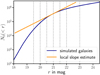Fig. 1. Cumulative number of galaxies N0 as a function of r-band magnitude for a field of 64 × 16 deg2 at redshift z = 0.41. The dotted vertical lines indicate the magnitude cuts listed in Table 1b. Finally, the tangential curve shows the local slope α at r = 21 mag.

4. Magnification effects on background galaxies

Lens and source galaxies are affected by magnification. To understand this impact in more detail, we first discuss how the shear profile changes when only source galaxies are magnified. In the following, we describe how we generated an arbitrary number of mock source catalogues, with and without magnification bias included. Results from the Millennium Simulations are then presented, and the magnification-induced bias in the GGL signal is compared to the prediction of the analytical model presented in Sect. 3.2.

4.1. Magnification switched off

To switch magnification off, we simply chose random source positions. We set the number of galaxies to N_s, 0 = 10⁷ per 16 deg² field to keep the impact of noise low.

4.2. Magnification switched on

Magnification changes the number counts of observed galaxies on the sky. Using the ray-tracing data, we obtained the cumulative number counts of the galaxies as a function of magnification-corrected flux, n_s, 0(> s₀). We obtained the local expected number counts of galaxies by adjusting the flux limit to s_lim, s/μ(θ) at each position θ and using the first equality in Eq. (15). We further scaled the number counts so that for μ = 1 the expected number of source galaxies is N_s = 10⁷ per field of solid angle A = 4° ×4°. The threshold of finding a source at a grid position θ is then T(θ) = n_s(> s_lim, s; θ) A/N_pix, where we restricted T(θ) to be smaller than unity. Finally, we drew a uniform random number P(θ) between zero and one for each position. A source galaxy was placed at a position θ if T(θ) > P(θ). The “magnification off” method can be recovered if we insert μ = 1 for all θ in Eq. (15).

4.3. Results

The relative impact of magnification of sources on a tangential shear profile is shown by the orange “upward” triangles in Fig. 2. As expected, the net effect depends on the local slope α_s; the effect is typically of the order of 1 to 2% per bin. In the two panels on the left-hand side in Fig. 2, the local slope α_s is larger than unity, and the shear signal is enhanced; while in the two panels on the right, α_s <  1, which reverses the effect. Also, the magnification effect is stronger for smaller separations θ. This is seen more clearly in Fig. 3, where the absolute difference of source-magnified to magnification-corrected shear profiles is compared. The shear profiles vary with α_s for constant redshifts z_d, s according to Table 1a. The difference between the expected and “measured” shear profiles in Fig. 3 is the bias that we estimated in Sect. 3.2 and gave in Eq. (16). We calculated the first and the third line of (16) using the numerical data and show them as solid and dotted lines, respectively. Both models are in good agreement with the numerical data for moderate α_s. However, for very steep α_s ≳ 2, the weak lensing approximation |μ − 1| ≪ 1 is not sufficient anymore; although large magnifications are rare, they affect the number counts significantly.

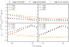Fig. 2. Relative difference between shear profiles with and without magnification. The redshifts for the lenses are zd = 0.41 in the upper panels and zd = 0.62 in the lower panels; the source redshift is kept fixed at zs = 0.99. The limiting magnitude of the lenses is 22 mag in the r-band, and for the sources it is 23 and 25 mag for αs = 1.75 and 0.58, respectively. The red “downward” triangles indicate shear profiles that only have magnification in the lens galaxy population, while the orange “upward” triangles show the influence of magnification for source galaxies only. It can be seen that a local slope > 1 of lens or source population leads to an enhanced signal, whereas αd, s <  1 causes a reduced signal. The green crosses display a measurement closest to real observations, i.e. where magnification affects both source and lens galaxy populations. A reduction or enhancement depends on both slopes αd, s, as well as the redshifts of lenses and sources zd, s. In all cases, the shape of the shear profile changes.

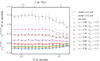Fig. 3. Absolute difference between shear profiles with and without magnification of sources, for different local slopes αs shown in the legend. The solid lines correspond to the first expression in Eq. (16) and dotted lines correspond to its approximation in the third line. The upper scale shows comoving transverse separation, and the redshifts are zs = 0.99 for the sources and zd = 0.41 for the lenses. The brown triangles with αs = 1.75 and the orange ones αs = 0.58 are directly comparable to the orange triangles in the upper panels of Fig. 2. We also show the goodness-of-fit parameter ${\chi }_{\text{red}}^2$ with 16 degrees of freedom for the solid line.

We define the mean fractional difference between a shear profile with and without magnification for all bins as

$$\begin{array}{c}\hfill {\delta }_{\gamma }=\frac{1}{N_{\mathrm{bin}}}{\displaystyle \sum _{i=1}^{N_{\mathrm{bin}}}\frac{{{\gamma }_{\mathrm{t}}}_i-{{\gamma }_{\mathrm{t}}}_i^{\mathrm{nomagn}}}{{{\gamma }_{\mathrm{t}}}_i^{\mathrm{nomagn}}},}\end{array}$$(20)

where we stress that a difference of δ_γ = 0 is not necessarily equivalent to an unaltered shear profile. However, we only applied this estimator to the orange “upward” and red “downward” triangles seen in Fig. 2, which display either a positive or a negative sign for all angular scales investigated.

Results for δ_γ as a function of α_s for constant z_s can be seen in Fig. 4. We selected the source galaxies according to Table 1a, for which δ_γ is almost linear in α_s, as expected from Eq. (16) in the weak lensing approximation, although the slope of the linear relation depends on different z_d (Table 1c). The maximum shear difference of 4% is found for the largest α_s.

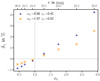Fig. 4. Fractional change of the shear profile by magnification, where the magnification is only turned on for the source galaxies at zs = 0.99 (Table 1a). At a local slope of αs ≈ 1 the impact of magnification flips its sign. The relation between αs and δγ is almost linear. Different redshifts of the lenses zd = 0.41 (plus) and 0.62 (cross) affect the impact of the sources’ magnification; the r-band limiting magnitude of lenses is fixed to 22 mag.

5. Magnification effects on foreground galaxies

In this section, we investigate the influence of magnification on lens galaxies. We follow the structure from the previous section, meaning we obtain and analyse results from the ray-tracing data and then compare those to the analytic estimate presented in Sect. 3.1.

5.1. Magnification switched on

The galaxies in the Henriques catalogue are affected by magnification by design. Hence, to create a catalogue including magnification, we simply extracted lens positions from galaxies brighter than a magnitude limit s_lim, d and assigned them to their nearest grid point.

5.2. Magnification switched off

To switch off magnification in the mock data, we undid the magnification as follows. As was done for the sources, the magnification-corrected flux s₀ can be easily recovered from the magnification given in the ray-tracing catalogue and the apparent flux of lens galaxies. The galaxy’s apparent position, however, is shifted on the sky compared to its unlensed position. Unfortunately, the unlensed position cannot be recovered from the simulated data, and the absolute amount of shifting is of the order of an arcminute and depends on redshift (Chang & Jain 2014). Hence, we must aim to create a sample of galaxies that is not affected by magnification in a different way.

As was outlined in Sect. 2.2, for both local slopes α_d, s = 1, the magnification leaves the observed number counts unaffected, and thus the shear profile γ_t unbiased. Therefore, we transformed the magnification-corrected flux distribution such that the galaxy counts obey $n_0^{\prime }\propto s_0^{\prime }{\text{}}^{-1}$. As a reference point, we chose the number of galaxies at limiting magnitude $n_0(>s_{\text{lim},\text{d}})=n_0^{\prime }(>s_{\text{lim},\text{d}}^{\prime })$. This results in the following mapping from observed magnification-corrected flux, s₀, to the transformed flux:

$$\begin{array}{c}\hfill s_0^{\prime }(s_0)=s_{\lim ,\mathrm{d}}\frac{n_0(s_{\lim ,\mathrm{d}})}{n_0(s_0)}·\end{array}$$(21)

In other words, this new flux scale distorts the number counts of lenses in such a way that in the transformed flux system, α′ = 1, the lens galaxy counts are unaffected by magnification bias (although the individual lens positions are not). We can now calculate the observed transformed number density n′( >  s′), where $s^{\prime }=\mu s_0^{\prime }$. To create a lens galaxy sample free from magnification, we again chose only those galaxies that are brighter than the given flux limit s′> s_lim, d. This leads to a different selection of galaxies for the original and the transformed number density.

We tested this approach with two consistency checks. The first is based on the fact that in the method described above, the total number of galaxies has to be conserved. This is true for all the lens redshifts used. For a magnitude cut of 22 mag in the r-band, a lens redshift of z_d = 0.41, and the full field of view of 64 × 16 deg², 595 348 lenses are found with a cut in observed magnitude, and 595 355 lenses are found with observed transformed magnitude. Compared to the original fluxes, a detailed analysis showed that in the transformed flux system, 917 galaxies became brighter than 22 mag, while 924 galaxies became dimmer, leaving the overall number count almost unchanged. The tiny difference in seven galaxies is due to the fact that the number count function is discretely sampled.

The second consistency check uses a null test: the so-called shear-ratio test (SRT, Jain & Taylor 2003), which is based on Eq. (18),

$$\begin{array}{c}\hfill T(\theta ;z_{\mathrm{d}},z_{{\mathrm{s}}_1},z_{{\mathrm{s}}_2}):=\frac{{\gamma }_{\mathrm{t}}(\theta ;z_{\mathrm{d}},z_{{\mathrm{s}}_1})}{{\gamma }_{\mathrm{t}}(\theta ;z_{\mathrm{d}},z_{{\mathrm{s}}_2})}-\frac{D_{{\mathrm{ds}}_1}}{D_{{\mathrm{s}}_1}}\frac{D_{{\mathrm{s}}_2}}{D_{{\mathrm{ds}}_2}},\end{array}$$(22)

for which we expect T(z_d, z_s1, z_s2) = 0 for two source populations at redshifts z_s1 and z_s2 in the absence of magnification effects. For the test, the location of the same lens galaxies and the shear from two source galaxy populations at different distances D_s1, 2 were used. A ratio of the tangential shear estimates is equal to the ratio of the corresponding angular-diameter distances, while the lens properties drop out. As shown in Unruh et al. (2019), the SRT is strongly affected by lens magnification. The impact is stronger for higher lens redshifts and smaller line-of-sight separation of lenses and sources. Therefore, we performed the SRT for lenses selected with and without magnification for two different lens redshifts. We performed the SRT by taking a weighted integral of T(θ; z_d, z_s1, z_s2) over θ from θ_in to θ_out as in Unruh et al. (2019). In the case that includes magnification, we recovered the results from Unruh et al. (2019). For lenses that are selected with corrected magnification, the SRT performs better by a factor of ≳100. We give results for two example redshift combinations in Table 2. The corrected SRT still shows a slight scatter due to the statistical noise in the data, coming from the lensing by the large-scale structure in each of the 64 fields, and a bias that arises from shifting lens galaxies to their nearest grid point.

5.3. Results

The red “downward” triangles in Fig. 2 show the relative impact of magnification on γ_t. Similar to the results given in Sect. 4.3, where the magnification of the source galaxies is discussed, the local slope α_d determines whether the shear signal is enhanced or reduced. The upper panels of Fig. 2 show that the shear profiles are reduced for a local slope α_d that is smaller than unity at redshift z_d = 0.42, while the lower panels display shear profiles with α_d >  1 at a higher redshift z_d = 0.62, where the reverse effect is observed. The panels with higher z_d show larger magnification effects; relative deviations by up to 7% in a single bin can be seen. In general, the shear signal is more strongly affected at larger separations θ from the lens centre until it reaches a maximum at ≈8′ for z_d = 0.62 and ≈10′ for z_d = 0.41; for even larger separations, the magnification effect becomes relatively weaker.

A comparison of numerical results to the analytic estimate (13) can be seen in Fig. 5. The absolute difference between shear profiles affected by a magnification of lens galaxies and those unaffected by magnification is plotted. The triangles show numerical results, while lines indicate our analytical model for $2[{\alpha }_{\mathrm{d}}(z_{\mathrm{d}})-1]{\gamma }_{\mathrm{t}}^{\mathrm{LSS}}$. We employed the reduced χ²-test as an estimator for the goodness of our model and find that all models are in good agreement with the data for the considered angular scales. However, the local slope is not necessarily a sufficiently good quantity for the analytic correction if the local slope α_d becomes very steep, meaning when the luminosity function is not well approximated by a power law anymore (cf. Fig. 1). However, the analytic correction still reduces the impact of magnification significantly.

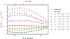Fig. 5. Absolute difference between shear profiles with and without magnification of lenses. The upper scale shows comoving transverse separation and the shear difference is shown for several limiting magnitudes of the lens galaxies, which yield the local slopes αd shown in the legend. Also, the goodness-of-fit parameter ${\chi }_{\text{red}}^2$ with 16 degrees of freedom is indicated in the legend. The redshifts are zs = 0.99 for the sources and zd = 0.41 for the lenses.

To explore the dependencies of the mean fractional shear difference δ_γ (Eq. (20)) on α_d, we altered the lens properties according to Table 1b. Results can be seen in Fig. 6 and show the impact of magnification for constant lens redshift z_d and varying limiting magnitude, for two different local slopes α_s of the sources. The impact on the shear profile is almost exactly the same in both local slopes, with a small residual noise that is present in the data. The dependence of δ_γ on α_d is similar to the one in Fig. 4, which shows the magnification for source galaxies only. The shear profile changes by up to 3% in the mean.

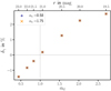Fig. 6. Behaviour of mean fractional shear difference δy as a function of local slope for lens galaxies αd and r-band-limiting magnitude, to change the lens properties according to Table 1b. The source and lens redshift is the same for both cases, i.e., zd = 0.41 and zs = 0.99. The effect is independent of the sources local slope αs.

We further investigated the dependence of the magnification on the values of α_d and z_d for fixed z_s in Fig. 7. δ_γ is calculated for various lens redshifts with constant limiting magnitude for the lenses (see Table 1c) and the same two values of α_s as before. The figure shows that the sources’ local slope does not affect the magnification induced by lens galaxies. The signal is again moderately reduced by 1% for α_d <  1 but is not monotonic anymore. For α_d >  1, the relation deviates significantly from a linear one. Magnification is stronger for larger α_d and larger z_d, leading to deviations of up to 45% in the most extreme case.

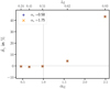Fig. 7. Impact on the shear profile as a function of αd and zd (Table 1c) for fixed flux limit of r = 22 mag, for a magnification of lens galaxies only. The redshift zd is given on the (non-linear) top axis. Again, the effect switches its sign at αd ≈ 1. It then rises up to 45% for larger αd, while less impact is seen for αd <  1. Different local slopes of the sources αs at zs = 0.99 leave the lens’ magnification unaffected.

Lastly, we combined the numerical methods and results that were addressed individually in Sects. 4 and 5. The green crosses in Fig. 2 show numerical results from source and lens galaxy populations that are both affected by magnification, meaning the case of relevance for observational studies of GGL. The fractional change is approximately the sum of the bias of lens galaxies only plus the bias of source galaxies only. Hence, to first order, it is determined by α_d and α_s. The sign of δ_γ cannot easily be predicted if α_d <  1 and α_s >  1, and vice versa. For δ_γ the sign also depends on θ since the change of shear signal per bin behaves differently for magnified lenses and magnified sources.

6. Magnification bias in halo-mass estimates

6.1. Estimating the mean halo mass of lenses

The GGL signal is sensitive to the surface-mass density around lenses that differs from the average projected cosmological matter density. To infer from this the mean mass of a parent halo that hosts a typical lens galaxy, we used a halo-model prescription to describe the relation between galaxies and matter (Cooray & Sheth 2002). In this prescription, we expand the galaxy-matter power spectrum at redshift z_d of lenses and at comoving wave number k,

$$\begin{array}{c}\hfill P_{\mathrm{gm}}(k)=P_{\mathrm{gm}}^{1\mathrm{h}}(k)+P_{\mathrm{gm}}^{2\mathrm{h}}(k),\end{array}$$(23)

in terms of a one-halo term,

$$\begin{array}{c}\hfill P_{\mathrm{gm}}^{1\mathrm{h}}(k)={\displaystyle {\int }_0^{\infty }\frac{\mathrm{d}mn(m)m}{{\mathrm{\Omega }}_{\mathrm{m}}{\rho }_{\mathrm{crit}}{\overline{n}}_{\mathrm{d}}}{\stackrel{\sim }{u}}_{\mathrm{m}}(k,m)(\langle N_{\mathrm{cen}}|m\rangle +\langle N_{\mathrm{sat}}|m\rangle {\stackrel{\sim }{u}}_{\mathrm{m}}(k,m)),}\end{array}$$(24)

and a two-halo term,

$$\begin{array}{cc}& P_{\mathrm{gm}}^{2\mathrm{h}}(k)={\displaystyle {\int }_0^{\infty }\frac{\mathrm{d}mn(m)m{b}_{\mathrm{h}}(m)}{{\mathrm{\Omega }}_{\mathrm{m}}{\rho }_{\mathrm{crit}}}{\stackrel{\sim }{u}}_{\mathrm{m}}(k,m)P_{\mathrm{lin}}(k)}\hfill \\ \hfill & \times {\displaystyle {\int }_0^{\infty }\frac{\mathrm{d}mn(m)b_{\mathrm{h}}(m)}{{\overline{n}}_{\mathrm{d}}}(\langle N_{\mathrm{cen}}|m\rangle +\langle N_{\mathrm{sat}}|m\rangle {\stackrel{\sim }{u}}_{\mathrm{m}}(k,m)).}\hfill \end{array}$$(25)

In this model, ${\stackrel{\sim }{u}}_{\mathrm{m}}(k,m)$ denotes the Fourier transform of a Navarro-Frenk-White (NFW; Navarro et al. 1996) density profile for a virial halo mass m, truncated at the virial radius and normalised to ${\stackrel{\sim }{u}}_{\mathrm{m}}(k,m)=1$ for k = 0 (Scoccimarro et al. 2001) for the mass-concentration relation in Bullock et al. (2001). We further denote the mean comoving number density of halos in the mass interval m₁ ≤ m <  m₂ by ${\int }_{m_1}^{m_2}\text{d}mn(m)$ (Sheth & Tormen 1999), the bias factor of halos of mass m by b_h(m) (Scoccimarro et al. 2001), and the linear matter power spectrum by P_lin(k) (Eisenstein & Hu 1998). Finally, the mean number density of lenses is

$$\begin{array}{c}\hfill {\overline{n}}_{\mathrm{d}}={\displaystyle {\int }_0^{\infty }\mathrm{d}mn(m)(\langle N_{\mathrm{cen}}|m\rangle +\langle N_{\mathrm{sat}}|m\rangle ).}\end{array}$$(26)

This version of the halo model assumes a central galaxy at the centre of a halo whenever there are lens galaxies inside the halo, and satellite galaxies with a number density profile equal to the NFW matter density. For the mean number of central and satellite galaxies for a halo mass m, we follow Clampitt et al. (2017) but with central-galaxy fraction f_cen ≡ 1,

$$\langle N_{\text{cen}}|m\rangle =\frac{1}{2}\left[1+\text{erf}\left(\frac{{\log }_{10}(m/m_{\text{th}})}{{\sigma }_{\log m}}\right)\right];$$(27)

$$\langle N_{\text{sat}}|m\rangle =\langle N_{\text{cen}}|m\rangle {\left(\frac{m}{m_1}\right)}^{\beta },$$(28)

where Θ = (m₁, m_th, σ _{log m}, β) are four model parameters that determine the halo-occupation distribution (HOD) of our lenses, and $\text{erf}(x)=2{\pi }^{-1/2}{\int }_0^x\text{d}t{\text{e}}^{-t^2}$ is the error function. The model parameters have the following meaning: m_th determines at which mass scale ⟨N_cen|m⟩ = 1/2; at halo mass m₁ the mean number of satellites equals that of central galaxies; σ _{log m} is the width of the HOD of centrals; and β is the slope of the satellite HOD.

The matter-galaxy cross-power spectrum is related to the mean tangential shear by a Limber projection, which for lenses at z_d and sources at z_s is

$$\begin{array}{c}\hfill {\gamma }_{\mathrm{t}}(\theta )=\frac{3H_0^2{\mathrm{\Omega }}_{\mathrm{m}}}{2c^2}\frac{D_{\mathrm{ds}}}{D_{\mathrm{d}}{D}_{\mathrm{s}}}{\displaystyle {\int }_0^{\infty }\frac{\mathrm{d}\ell \ell }{2\pi }{J}_2(\ell \theta )P_{\mathrm{gm}}(\frac{\ell +1/2}{(1+z_{\mathrm{d}})D_{\mathrm{d}}};z_{\mathrm{d}}).}\end{array}$$(29)

We employed a maximum-likelihood estimator (MLE) to infer the mean halo mass of lenses from GGL. For this, we set {γ_t, i(Θ)|i = 1…N_bin} as a set of N_bin measurements of the mean tangential shear in our mock data, obtained for different lens-source angular separation bins i; the error covariance estimated from the measurements for bin θ_i and θ_j is C_ij, and its inverse [C⁻¹]_ij. For the MLE of Θ, we then minimised

$$\begin{array}{c}\hfill {\chi }^2(\mathbf{\Theta })={\displaystyle \sum _{i,j=1}^{N_{\mathrm{bin}}}({\gamma }_{\mathrm{t},i}(\mathbf{\Theta })-{\gamma }_{\mathrm{t},i}){[{\mathsf{C}}^{-1}]}_{\mathit{ij}}({\gamma }_{\mathrm{t},j}(\mathbf{\Theta })-{\gamma }_{\mathrm{t},j}),}\end{array}$$(30)

with respect to Θ, where γ_t, i(Θ) is the halo model prediction of γ_t(θ|Θ) averaged over the size of the ith separation bin that corresponds to γ_t, i. We refer to Θ_mle as the parameter set that minimises χ²(Θ). Finally, given the MLE Θ_mle, we obtain the MLE of the mean halo mass by the integral

$$\begin{array}{c}\hfill {\langle m\rangle }_{\mathrm{mle}}={\displaystyle {\int }_0^{\infty }\frac{\mathrm{d}mn(m)m}{{\overline{n}}_{\mathrm{d}}}(\langle N_{\mathrm{cen}}|m\rangle +\langle N_{\mathrm{sat}}|m\rangle ),}\end{array}$$(31)

which has to be evaluated for the HOD of galaxies that is determined by Θ_mle.

In Fig. 8, we show four examples of tangential shear estimates and their best shear profile fit from the halo model. For the shear profiles, we switched off magnification effects of lens and source galaxies. It can be seen that the fitting procedure works reasonably well. The halo model itself is only an approximation of the inhomogeneous matter distribution in the Universe, and in the presence of our simulated data with almost vanishing Poisson noise, we do not expect the halo model to work perfectly. We further used approximations such as a truncated NFW model and a specific mass-concentration relation, that certainly further limits the accuracy we can obtain with the halo model. The mean relative difference between the data and the model for the 16 bins is 2.6% for z_d = 0.41, and 1.3% for z_d = 0.62. As expected, the shear profiles are almost independent of the flux limit of sources if their redshift is fixed, as can be seen for the red and blue crosses, as well as for the magenta and green crosses. On the other hand, there are three main reasons for the difference between the red/blue and magenta/green shear profiles. The lensing efficiencies D_ds/D_s are different for different z_d. Thus, the red/blue shear profile with z_d = 0.41 has a larger lensing efficiency than the magenta/green one with z_d = 0.62. Moreover, we observed fixed angular scales, which corresponds to different physical scales. Lastly, the lens galaxy population might evolve between the two redshifts.

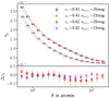Fig. 8. Upper panel: magnification-corrected shear profiles for two lens redshifts zd with a r-band magnitude cut of 22 mag and two differently selected source galaxies at redshift zs = 0.99 (crosses) as well as their best fit according to the halo model (solid line). Lower panel: absolute difference Δγt between data and halo model fit (open circles with the same colour). For each lens redshift, source galaxies were chosen with two limiting magnitudes that have the local slopes αs = 0.58 and 1.75, respectively. As expected, the shear profile does not depend on the choice of source galaxies. The offset between the red/blue points as well as the magenta/green points is for better visibility only.

Table 3 accompanies Fig. 8 and lists the fitting parameters, the goodness-of-fit values, and the mass estimates for the different shear profiles. The mean halo mass, in contrast to the shear amplitude, is larger for the high-redshift lenses when the same magnitude limit is applied.

We quantify this bias in halo mass for fixed limiting magnitudes of lenses and sources, which means fixed α_d, s, and fixed redshifts as follows. Using the halo model as described above, we calculated the best mass estimate from the magnification-corrected shear profile. As could be seen in the previous sections, the relative change of the shear profile is typically of the order of a couple of percent. Therefore, we fixed the scatter in the host halo mass σ _{log m} and the slope of the mean number of satellite galaxies β to their best fit value in the magnification-corrected case. Then, we only fitted the remaining two parameters m_th and m₁ to estimate the mass for the three remaining shear profiles, meaning a shear profile with magnification of the sources only turned on, a profile with magnification of the lenses only turned on, and a shear profile with lens and source magnification turned on. Similar to the fractional shear difference (20), we define the bias of halo-mass estimates, inferred from γ_t, by

$$\begin{array}{c}\hfill {\delta }_{\mathrm{M}}=\frac{{\langle m\rangle }_{\mathrm{mle}}-{\langle m\rangle }_{\mathrm{mle}}^{\mathrm{nomagn}}}{{\langle m\rangle }_{\mathrm{mle}}^{\mathrm{nomagn}}}·\end{array}$$(32)

6.2. Numerical results

Figures 9–12 show results for the mass bias δ_M. Figure 9 shows the bias for magnified source galaxy counts and magnification-corrected lens counts. The lenses have constant limiting magnitude of 22 mag in the r-band and their redshifts are z_d = 0.41 and 0.62. Source galaxies at redshift z_s = 0.99 are selected for several limiting magnitudes (cf. Table 1a). The bias is of the same order of magnitude as the corresponding mean fractional difference of the shear, and α_s determines whether mass is overestimated or underestimated. The mean halo mass is biased by up to 3.5%.

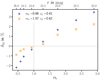Fig. 9. Relative mass bias δM (32) for magnified source number counts. Source galaxies are at zs = 0.99 and lenses are chosen according to Table 1a with redshifts zd = 0.41 (plus) and 0.62 (cross), for fixed limiting magnitude. The mass bias behaves roughly like the fractional shear difference (cf. Fig. 4). For local slopes αs <  1, the underestimation of mass is stronger than for the shear profile, while for αs >  1 the overestimate is similar.

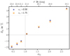Fig. 10. Fractional mass bias δM shown as a function of local slope αd and r-band limiting magnitude (cf. Table 1b). The source redshift is zs = 0.99 and lens redshift is zd = 0.41. For αd <  1, δM the mass is biased low, while for αd >  1 the mass is biased high.

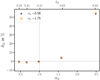Fig. 11. The fractional mass bias δM is shown as a function of local slope αd and lens redshift zd (cf. Table 1c). We keep the r-band limiting magnitude for the lenses and the source redshift zs = 0.99 constant. The top axis indicates the respective lens redshifts in a non-linear scaling. Following the trend seen in Fig. 7, mass is biased low for αd < 1 and shows large biases for αd > 1.

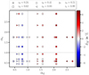Fig. 12. Total magnification bias for halo-mass estimates as a function of limiting magnitudes that yield the local slopes αd, s and lens redshift zd (type of symbols). The source redshift is the same in all cases, i.e., zs = 0.99. The mass difference δM is shown in colour code, where blue indicates underestimation, red overestimation, and white is an unbiased result. We cut off the colour bar for the largest deviations of 55% and 58% for αd = 2.41 and zd = 0.83 for higher contrast in the colour scale. The plot is roughly divided by the vertical line with αd = 1 into mass underestimation for αd <  1 and overestimation αd >  1.

We then explored the dependencies of the fractional mass bias δ_M on α_d, while we only considered magnification-corrected sources. Firstly, we fixed the lens redshift to z_d = 0.41 and altered the lens’ limiting magnitude according to Table 1b. The result is shown in Fig. 10. The mass bias is an almost linear function of α_d and shows a similar dependence on α_d as the fractional shear difference (cf. Fig. 6). The mass is biased up to 5% for the largest α_d. Lastly, we calculated δ_M for various lens redshifts with constant limiting magnitude for the lenses (see Table 1c) and the same two α_s as before, which is shown in Fig. 11. The mass bias shows a strong redshift dependence, where the bias increases from a couple of percent to a mass overestimate of 55%.

To explore the observationally relevant case, we compared halo-mass estimates with and without magnification for both lenses and sources. Figure 12 contains all different α_d, s − z_d combinations with constant z_s = 0.99 from Tables 1a–c, plus some additional combinations. It shows δ_M as defined in Eq. (32) as a function of the local slopes α_d, s on the x- and y-axis. Red values indicate an overestimation of the mass, where we cut off the colour bar for the highest values for better visibility. The blue values show an underestimation, while white values mean no bias in the mass estimate. The upper-right quadrant shows consistently red values since α_d, s >  1, while the lower-left quadrant has α_d, s <  1 and is consistently blue, as expected from theoretical considerations. In most of the other cases, α_d seems to be the decisive factor for the sign of the mass bias, for α_d <  1 leading to an underestimation and for α_d >  1 leading to an overestimation. The slope α_s influences the total value of the mass bias. Besides, even if two points are close in the α_d − α_s parameter space, they do not exhibit the same colour, meaning mass bias, due to their different z_d.

7. Discussion and conclusions

In this paper, we quantified the impact of magnification on the GGL signals and halo-mass estimates. Magnification changes the observed galaxy number counts on the sky, which has an impact on the measured tangential shear profiles. It is important to note that magnification affects lens galaxies as well as source galaxies. Analyses of tangential shear profiles, such as estimates of the excess mass density profiles or halo mass, are therefore biased if they ignore lens or source magnification. Our estimates with ray-tracing simulations and synthetic galaxy populations show that the number count slopes of sources and lenses are the most important quantities that determine the relative strength of the bias. While the analytical estimate for the bias on the GGL profile caused by magnification of lenses was known before, to our knowledge the one caused by magnification of the source population has not previously been derived.

How magnification affects tangential shear profiles can be seen in Figs. 2–7, where we varied the local slope of lens and sources galaxies α_d, s and the lens redshift z_d. We studied the magnification effect from lenses and sources individually and compared them to our analytic estimates. The latter are leading-order estimates and describe the numerical results very well in most cases. One of the surprising results, shown in Fig. 3, is that the weak lensing approximation for the impact of magnification on source counts can significantly fail if the count slope is steep. Hence, the validity of the commonly used approximation for the number density of sources

$$\begin{array}{c}\hfill n_{\mathrm{s}}(\mathit{\theta },>s)\approx n_{\mathrm{s}0}(>s)[1+2({\alpha }_{\mathrm{s}}-1)\kappa (\mathit{\theta })]\end{array}$$

needs to be checked, depending on its application.

Besides confirming that the shear signal is reduced if the slopes α_d and α_s are < 1 and enhanced for α_d, s >  1, we find: For fixed redshifts z_d, s, the change of the tangential shear estimate depends solely on α_d, s. For fixed source redshifts z_s, the impact of magnification of sources decreases for larger z_d and smaller lens-source separation D_ds (cf. Fig. 4). Furthermore, the relative importance of magnification of lenses increases with z_d and rises sharply as z_d approaches z_s. The relative change from a biased to an unbiased shear profile is a function of angular separation θ, and the mean change is typically a few percent. However, if the redshift differences between sources and lenses become small, the effect can be considerably larger (cf. Fig. 7).

For practical applications, the change in the shear signal by magnification is described by the sum of the individual effects of source magnification and the one from lens magnification. The impact of magnification depends on the galaxy’s luminosity function, the limiting magnitudes, and the redshifts z_d, s, but also the separation θ.

The relative mass bias δ_M on the average mass of a lens parent-halo inherits all trends seen in the shear profiles with magnified lenses and magnified sources (see Figs. 9–12), meaning δ_M >  0 for α_d, s >  0 and vice versa. Medium-redshift galaxies show a mass bias of less than 10%, and the higher the lens redshift, the stronger the mass bias with up to 58% for z_d = 0.83 and z_s = 0.99. The bias δ_M is of the same order of magnitude as the relative change of the shear profile δ_γ. The particular relation, however, between δ_γ and the mass bias δ_M is quite complicated. First and foremost, the amplitude of the measured shear signal determines the underlying halo mass. However, magnification changes the scale dependence of the shear signal. In the halo model, this translates to a different behaviour of the one- and two-halo term, which affects the mass estimate in a highly non-linear way. Another minor effect is that the true mean halo mass of lens galaxies affected by magnification probably differs from the true mean halo mass of unmagnified lenses due to an expected correlation between mass and luminosity. For example, for the highest z_d considered in this work, the mean masses differ by 0.16%. Furthermore, we fixed the observed angular scales on the sky, which relate to different physical scales at different redshifts; thus, the relative contribution of the two-halo term on the shear signal grows with redshift, which makes a comparison of mass biases from different lens redshifts more complicated. In general, when we allow for magnification effects both in source and lens galaxies, meaning, the case for real observations, the sign of the mass bias is in most cases determined by the value of α_d. The only exceptions shown in Fig. 12 are two cases, where either the lens redshift is low or the local slope α_s is very high; in such cases, the sign of the mass bias is not easily predicted and must be studied case by case.

We also considered a GGL estimate using the flux-limits and redshift distributions as given from the combined data of KiDS+VIKING (Hildebrandt et al. 2020) and GAMA (Driver et al. 2011). KiDS and VIKING are partner surveys that probe the optical and near-infrared sky to obtain high-resolution, wide-field shape and redshift information from galaxies. GAMA is a spectroscopic, flux-limited survey with a partly overlapping footprint in the KiDS+VIKING area. In Appendix A.3, we present a detailed description of the input parameters we use for this estimate. We list the results in Table A.1. A lens galaxy sample at redshift z_d = 0.21 shows relative changes in the shear profile due to magnification effects of less than one percent, and relative mass bias of ≈3%, while GAMA’s highest lens sample at z_d = 0.36 shows that a magnification correction changes the shear profile by ≈2% and the relative halo mass bias by 8%. Although our estimate used simplifying assumptions, especially for the source population, for example, no catastrophic outliers in the redshift distribution and no further selection criteria than a cut in magnitude, we conclude that magnification effects must be carefully considered in current and future surveys.

In this paper, we assume that lenses and sources form a flux-limited sample. While this assumption may be a realistic one for lens galaxies (e.g. galaxy redshift surveys frequently start from a flux-limited photometric sample), it is less the case for source galaxies. Sources in weak lensing studies have rather complicated selection criteria, not merely based on flux, but also on size and signal-to-noise ratio, for example. Therefore, our quantitative analysis may not apply directly to observational surveys. Besides, source galaxies typically enter a weak lensing catalogue with a weight that characterises the accuracy of the corresponding shear estimate. We ignored any such weighting scheme in our processing, but it may be relevant, since the weight of an object is also expected to depend on magnitude and size, and is thus affected by magnification.

While the relative amplitude of the bias caused by magnification is modest in most cases, and probably smaller than the uncertainties from shape noise and sample variance in previous surveys, future surveys like Euclid or LSST have such improved statistical power that magnification effects must be accounted for in the quantitative analysis of GGL.

Acknowledgments

The authors would like to thank the anonymous referee for his constructive and helpful comments that improved the quality of this paper. Part of this work was supported by the Deutsche Forschungsgemeinschaft, DFG project number SCHN 342/13-1. Sandra Unruh is a member of the International Max Planck Research School (IMPRS) for Astronomy and Astrophysics at the Universities of Bonn and Cologne.Stefan Hilbert acknowledges support by the DFG cluster of excellence “Origin and Structure of the Universe” (www.universe-cluster.de).

References

Appendix A: Mock data

A.1 Millennium Simulation data

To study magnification effects in GGL, we make use of ray-tracing results through the Millennium Simulation (MS, Springel 2005), which is an N-body simulation of 2160³ dark matter particles. Each particle has a mass of 8.6 × 10⁸h⁻¹ M_⊙ that is confined to a cube with side length of 500 h⁻¹ Mpc and with periodic boundary conditions. The underlying cosmology is a flat ΛCDM model with a matter density parameter of Ω_m = 0.25, a baryon density parameter of Ω_b = 0.045, a dimensionless Hubble parameter of h = 0.73, a tilt of the primordial power spectrum of n = 1, and a variance of matter fluctuations on a scale of 8 h⁻¹ Mpc extrapolated from a linear power spectrum of σ₈ = 0.9. This cosmology is based on combined results of 2dFGRS (Colless et al. 2001) and first-year WMAP data (Spergel et al. 2003).

The ray-tracing results are based on a multiple-lens-plane algorithm in 64 light cones constructed from 37 snapshots between redshifts z = 0 to z = 3.06, each covering a 4 × 4 deg² field of view. For more information about the ray tracing, the reader is kindly referred to Hilbert et al. (2009). An important aspect of the algorithm is that the galaxy-matter correlation is preserved. The ray-tracing results contain the Jacobians 𝒜 on a N_pix = 4096² pixel grid, which corresponds to a resolution of 3.5 arcsec per pixel. From this, we calculated shear and magnification on a pixel grid.

We also used a catalogue of galaxies based on a semi-analytic galaxy-formation model by Henriques et al. (2015). This catalogue matches the GGL and galaxy-galaxy-galaxy lensing signal from CFHTLenS (Saghiha et al. 2017). The galaxies are listed for each redshift snapshot with various properties, for example, (magnified) flux in various filters and positions, which allows for selection according to chosen magnitude limits. However, the galaxy positions are not confined to a grid as is the Jacobi information. Thus, we shifted all selected galaxies to their nearest grid point. Therefore, analyses that are close to the centre of the galaxy suffer from discretisation effects on scales comparable to the pixel size.

A.2 Obtaining a tangential shear estimate

To extract the shear signal averaged over many lenses, a fast Fourier transform (FFT) is employed. In order to do so, we first defined lens and source number density on a grid by

$$\begin{array}{c}\hfill n_{\mathrm{d},\mathrm{s}}(\mathit{\theta })={\displaystyle \sum _{i=1}^{N_{\mathrm{d},\mathrm{s}}}}{\delta }_{\mathrm{K}}(\mathit{\theta }-{\mathit{\theta }}_{\mathrm{d},\mathrm{s}}^{(i)}),\end{array}$$(A.1)

with δ_K being one if $\mathit{\theta }={\mathit{\theta }}_{\mathrm{d},\mathrm{s},}^{(i)}$ and zero otherwise. The number of lenses and sources is N_d, s, and ${\mathit{\theta }}_{\mathrm{d},\mathrm{s}}^{(i)}$ are the positions of lenses and sources, respectively. Furthermore, we define the shear field of the sources on the grid by

$$\begin{array}{c}\hfill {\gamma }_{\mathrm{s}}(\mathit{\theta })={\displaystyle \sum _{i=1}^{N_{\mathrm{s}}}}\gamma (\mathit{\theta },z_{\mathrm{s}}){\delta }_{\mathrm{K}}(\mathit{\theta }-{\mathit{\theta }}_{\mathrm{s}}^{(i)}).\end{array}$$(A.2)

Then, the tangential shear estimator (11) can be expressed as

$$\begin{array}{c}\hfill {\widehat{\gamma }}_{\mathrm{t}}(\theta )=-\mathfrak{R}\frac{{\sum }_{{\mathit{\theta }}^{\prime }}\mathrm{\Delta }(\theta ,|{\mathit{\theta }}^{\prime }|){\mathit{\theta }}^{\prime \ast }/{\mathit{\theta }}^{\prime }{\sum }_{{\mathit{\theta }}^{″}}{n}_{\mathrm{d}}({\mathit{\theta }}^{″}){\gamma }_{\mathrm{s}}({\mathit{\theta }}^{″}+{\mathit{\theta }}^{\prime })}{{\sum }_{{\mathit{\theta }}^{\prime }}\mathrm{\Delta }(\theta ,|{\mathit{\theta }}^{\prime }|){\sum }_{{\mathit{\theta }}^{″}}{n}_{\mathrm{d}}({\mathit{\theta }}^{″})n_{\mathrm{s}}({\mathit{\theta }}^{″}+{\mathit{\theta }}^{\prime })},\end{array}$$(A.3)

where the sums over θ′ and θ″ extend over the whole grid. The equivalence of Eqs. (A.3) and (11) can be verified by inserting the definitions of n_d, s and γ_s into the former. The sum over θ″ in the denominator calculates for each θ′ the number of lens-source pairs, ensuring that (A.3) is not affected by a potential masking or inhomogeneous survey areas. Further, the sums over θ″ in the numerator and denominator of the GGL estimator (A.3) are convolutions. Thus, the convolution theorem can be applied to these sums. If ℱ{f} is the Fourier transform of a function f and ℱ⁻¹ the inverse Fourier transform, then we can rewrite the estimator (A.3) as

$$\begin{array}{c}\hfill {\widehat{\gamma }}_{\mathrm{t}}(\theta )=-\mathfrak{R}\frac{{\sum }_{{\mathit{\theta }}^{\prime }}\mathrm{\Delta }(\theta ,|{\mathit{\theta }}^{\prime }|){\mathit{\theta }}^{\prime \ast }/{\mathit{\theta }}^{\prime }{\mathcal{F}}^{-1}\left\{\mathcal{F}\left\{n_{\mathrm{d}}\right\}\mathcal{F}\left\{{\gamma }_{\mathrm{s}}\right\}({\mathit{\theta }}^{\prime })\right\}}{{\sum }_{{\mathit{\theta }}^{\prime }}\mathrm{\Delta }(\theta ,|{\mathit{\theta }}^{\prime }|){\mathcal{F}}^{-1}\left\{\mathcal{F}\left\{n_{\mathrm{d}}\right\}\mathcal{F}\left\{n_{\mathrm{s}}\right\}\right\}({\mathit{\theta }}^{\prime })},\end{array}$$(A.4)

which can be readily solved by an FFT method. For this, we employed routines from the FFTW library by Frigo & Johnson (2005) in our code.

A FFT implicitly assumes periodic boundary conditions, which introduces a bias to the averaged shear data and, thus, must be mitigated for. We can restrict the selection of lenses to the inner (4° −2θ_out)² of the field, where θ_out is the maximum separation from the lens that we considered. However, for a θ_out ≈ 20′, we already lose approximately 30% of the lens galaxies. Alternatively, we employed a zero-padding method in which we increased the FFT-area to (4° +θ_out)² and filled the added space with zeros. In this case, we used all available lenses with the cost of slightly increased computational time and the gain of a less-noisy shear profile. For the whole 64 × 16 deg², our FFT-based code needs a CPU time of 823 s, independent of the number of sources and lenses. We compared the performance of our method to the publicly available athena tree-code (Kilbinger et al. 2014). In contrast to the FFT method, the computation time of athena is enhanced with the number of lens-source pairs. We adjusted the settings to our survey parameters while leaving the parameter that sets the accuracy of the tree-code, meaning the open-angle threshold, to its pre-set value. For 10⁷ sources and lenses at z_d = 0.41 with limiting magnitudes 19.5, 22, and 29 mag, athena performs with a CPU time of 889 s, 1167 s, and 2043 s, respectively.

A.3 Estimating the impact of the magnification bias on a KiDS+VIKING+GAMA-like survey

We considered GAMA-like lens galaxies with narrow redshift distributions at z_d = 0.21 and z_d = 0.36 with a flux limit of 19.8 mag. Using simulated data from the semi-analytic galaxy-formation model by Henriques et al. (2015), we obtain local slopes of α_d = 0.85 and α_d = 2.11, respectively. To keep the statistical error low, we still consider the data from the whole simulated area of 64 × 16 deg². To mimic the KiDS+VIKING-like source population, we matched the last three bins of the best-estimated redshift distribution to Millennium data from 0.51 ≤ z_s, Mil <  1.28. We then calculated a weighted shear map from the simulated data, the final source galaxy distribution has a local slope of α_s = 0.51 for a limiting magnitude of 25 mag. We repeated our analysis from Sects. 4–6, and obtain the results listed in Table A.1. The results are quantitatively comparable to the results from Figs. 4 and 6.

A KiDS+VIKING+GAMA-like survey is moderately affected. We stress that this estimate has been made with simplified assumptions, for example, there are no catastrophic outliers in the redshift distribution and no selection criteria for source galaxies other than a magnitude cut.

All Tables

All Figures

	Fig. 1. Cumulative number of galaxies N0 as a function of r-band magnitude for a field of 64 × 16 deg2 at redshift z = 0.41. The dotted vertical lines indicate the magnitude cuts listed in Table 1b. Finally, the tangential curve shows the local slope α at r = 21 mag.
In the text

Fig. 2. Relative difference between shear profiles with and without magnification. The redshifts for the lenses are zd = 0.41 in the upper panels and zd = 0.62 in the lower panels; the source redshift is kept fixed at zs = 0.99. The limiting magnitude of the lenses is 22 mag in the r-band, and for the sources it is 23 and 25 mag for αs = 1.75 and 0.58, respectively. The red “downward” triangles indicate shear profiles that only have magnification in the lens galaxy population, while the orange “upward” triangles show the influence of magnification for source galaxies only. It can be seen that a local slope > 1 of lens or source population leads to an enhanced signal, whereas αd, s <  1 causes a reduced signal. The green crosses display a measurement closest to real observations, i.e. where magnification affects both source and lens galaxy populations. A reduction or enhancement depends on both slopes αd, s, as well as the redshifts of lenses and sources zd, s. In all cases, the shape of the shear profile changes.

In the text

Fig. 3. Absolute difference between shear profiles with and without magnification of sources, for different local slopes αs shown in the legend. The solid lines correspond to the first expression in Eq. (16) and dotted lines correspond to its approximation in the third line. The upper scale shows comoving transverse separation, and the redshifts are zs = 0.99 for the sources and zd = 0.41 for the lenses. The brown triangles with αs = 1.75 and the orange ones αs = 0.58 are directly comparable to the orange triangles in the upper panels of Fig. 2. We also show the goodness-of-fit parameter ${\chi }_{\text{red}}^2$ with 16 degrees of freedom for the solid line.

In the text

Fig. 4. Fractional change of the shear profile by magnification, where the magnification is only turned on for the source galaxies at zs = 0.99 (Table 1a). At a local slope of αs ≈ 1 the impact of magnification flips its sign. The relation between αs and δγ is almost linear. Different redshifts of the lenses zd = 0.41 (plus) and 0.62 (cross) affect the impact of the sources’ magnification; the r-band limiting magnitude of lenses is fixed to 22 mag.

In the text

Fig. 5. Absolute difference between shear profiles with and without magnification of lenses. The upper scale shows comoving transverse separation and the shear difference is shown for several limiting magnitudes of the lens galaxies, which yield the local slopes αd shown in the legend. Also, the goodness-of-fit parameter ${\chi }_{\text{red}}^2$ with 16 degrees of freedom is indicated in the legend. The redshifts are zs = 0.99 for the sources and zd = 0.41 for the lenses.

In the text

	Fig. 6. Behaviour of mean fractional shear difference δy as a function of local slope for lens galaxies αd and r-band-limiting magnitude, to change the lens properties according to Table 1b. The source and lens redshift is the same for both cases, i.e., zd = 0.41 and zs = 0.99. The effect is independent of the sources local slope αs.
In the text

Fig. 7. Impact on the shear profile as a function of αd and zd (Table 1c) for fixed flux limit of r = 22 mag, for a magnification of lens galaxies only. The redshift zd is given on the (non-linear) top axis. Again, the effect switches its sign at αd ≈ 1. It then rises up to 45% for larger αd, while less impact is seen for αd <  1. Different local slopes of the sources αs at zs = 0.99 leave the lens’ magnification unaffected.

In the text

Fig. 8. Upper panel: magnification-corrected shear profiles for two lens redshifts zd with a r-band magnitude cut of 22 mag and two differently selected source galaxies at redshift zs = 0.99 (crosses) as well as their best fit according to the halo model (solid line). Lower panel: absolute difference Δγt between data and halo model fit (open circles with the same colour). For each lens redshift, source galaxies were chosen with two limiting magnitudes that have the local slopes αs = 0.58 and 1.75, respectively. As expected, the shear profile does not depend on the choice of source galaxies. The offset between the red/blue points as well as the magenta/green points is for better visibility only.

In the text

Fig. 9. Relative mass bias δM (32) for magnified source number counts. Source galaxies are at zs = 0.99 and lenses are chosen according to Table 1a with redshifts zd = 0.41 (plus) and 0.62 (cross), for fixed limiting magnitude. The mass bias behaves roughly like the fractional shear difference (cf. Fig. 4). For local slopes αs <  1, the underestimation of mass is stronger than for the shear profile, while for αs >  1 the overestimate is similar.

In the text

	Fig. 10. Fractional mass bias δM shown as a function of local slope αd and r-band limiting magnitude (cf. Table 1b). The source redshift is zs = 0.99 and lens redshift is zd = 0.41. For αd <  1, δM the mass is biased low, while for αd >  1 the mass is biased high.
In the text

	Fig. 11. The fractional mass bias δM is shown as a function of local slope αd and lens redshift zd (cf. Table 1c). We keep the r-band limiting magnitude for the lenses and the source redshift zs = 0.99 constant. The top axis indicates the respective lens redshifts in a non-linear scaling. Following the trend seen in Fig. 7, mass is biased low for αd < 1 and shows large biases for αd > 1.
In the text

Fig. 12. Total magnification bias for halo-mass estimates as a function of limiting magnitudes that yield the local slopes αd, s and lens redshift zd (type of symbols). The source redshift is the same in all cases, i.e., zs = 0.99. The mass difference δM is shown in colour code, where blue indicates underestimation, red overestimation, and white is an unbiased result. We cut off the colour bar for the largest deviations of 55% and 58% for αd = 2.41 and zd = 0.83 for higher contrast in the colour scale. The plot is roughly divided by the vertical line with αd = 1 into mass underestimation for αd <  1 and overestimation αd >  1.

In the text

References

- Bartelmann, M., & Schneider, P. 2001, Phys. Rep., 340, 291 [NASA ADS] [CrossRef] [Google Scholar]
- Bullock, J. S., Kolatt, T. S., Sigad, Y., et al. 2001, MNRAS, 321, 559 [Google Scholar]
- Chang, C., & Jain, B. 2014, MNRAS, 443, 102 [CrossRef] [Google Scholar]
- Chiu, I., Dietrich, J. P., Mohr, J., et al. 2016, MNRAS, 457, 3050 [CrossRef] [Google Scholar]
- Clampitt, J., Sánchez, C., Kwan, J., et al. 2017, MNRAS, 465, 4204 [NASA ADS] [CrossRef] [Google Scholar]
- Colless, M., Dalton, G., Maddox, S., et al. 2001, MNRAS, 328, 1039 [NASA ADS] [CrossRef] [Google Scholar]
- Cooray, A., & Sheth, R. 2002, Phys. Rep., 372, 1 [NASA ADS] [CrossRef] [Google Scholar]
- Driver, S. P., Hill, D. T., Kelvin, L. S., et al. 2011, MNRAS, 413, 971 [NASA ADS] [CrossRef] [Google Scholar]
- Eisenstein, D. J., & Hu, W. 1998, ApJ, 496, 605 [NASA ADS] [CrossRef] [Google Scholar]
- Frigo, M., & Johnson, S. G. 2005, Proc. IEEE, 93, 216 [Google Scholar]
- Garcia-Fernandez, M., Sanchez, E., Sevilla-Noarbe, I., et al. 2018, MNRAS, 476, 1071 [NASA ADS] [CrossRef] [Google Scholar]
- Hartlap, J. 2009, PhD Thesis, AIfA – Argelander-Institut für Astronomie, Rheinische Friedrich-Wilhelms Universität Bonn, Germany [Google Scholar]
- Henriques, B. M. B., White, S. D. M., Thomas, P. A., et al. 2015, MNRAS, 451, 2663 [NASA ADS] [CrossRef] [Google Scholar]
- Hilbert, S., Hartlap, J., White, S. D. M., & Schneider, P. 2009, A&A, 499, 31 [NASA ADS] [CrossRef] [EDP Sciences] [Google Scholar]
- Hildebrandt, H., Köhlinger, F., van den Busch, J. L., et al. 2020, A&A, 633, A69 [NASA ADS] [CrossRef] [EDP Sciences] [Google Scholar]
- Hoekstra, H. 2013, ArXiv e-prints [arXiv:1312.5981] [Google Scholar]
- Jain, B., & Taylor, A. 2003, Phys. Rev. Lett., 91, 141302 [NASA ADS] [CrossRef] [PubMed] [Google Scholar]
- Kilbinger, M. 2015, Rep. Prog. Phys., 78, 086901 [Google Scholar]
- Kilbinger, M., Bonnett, C., & Coupon, J. 2014, Astrophysics Source Code Library [ascl:1402.026] [Google Scholar]
- Kilbinger, M., Heymans, C., Asgari, M., et al. 2017, MNRAS, 472, 2126 [NASA ADS] [CrossRef] [Google Scholar]
- Navarro, J. F., Frenk, C. S., & White, S. D. M. 1996, ApJ, 462, 563 [NASA ADS] [CrossRef] [Google Scholar]
- Saghiha, H., Simon, P., Schneider, P., & Hilbert, S. 2017, A&A, 601, A98 [NASA ADS] [CrossRef] [EDP Sciences] [Google Scholar]
- Schneider, P., & Watts, P. 2005, A&A, 432, 783 [NASA ADS] [CrossRef] [EDP Sciences] [Google Scholar]
- Scoccimarro, R., Sheth, R. K., Hui, L., & Jain, B. 2001, ApJ, 546, 20 [NASA ADS] [CrossRef] [Google Scholar]
- Sheth, R. K., & Tormen, G. 1999, MNRAS, 308, 119 [NASA ADS] [CrossRef] [Google Scholar]
- Simon, P., & Hilbert, S. 2018, A&A, 613, A15 [NASA ADS] [CrossRef] [EDP Sciences] [Google Scholar]
- Simon, P., Watts, P., Schneider, P., et al. 2008, A&A, 479, 655 [NASA ADS] [CrossRef] [EDP Sciences] [Google Scholar]
- Simon, P., Erben, T., Schneider, P., et al. 2013, MNRAS, 430, 2476 [NASA ADS] [CrossRef] [EDP Sciences] [Google Scholar]
- Singh, S., Mandelbaum, R., Seljak, U., Slosar, A., & Vazquez Gonzalez, J. 2017, MNRAS, 471, 3827 [NASA ADS] [CrossRef] [Google Scholar]
- Spergel, D. N., Verde, L., Peiris, H. V., et al. 2003, ApJS, 148, 175 [NASA ADS] [CrossRef] [Google Scholar]
- Springel, V. 2005, MNRAS, 364, 1105 [NASA ADS] [CrossRef] [Google Scholar]
- Takahashi, R., Sato, M., Nishimichi, T., Taruya, A., & Oguri, M. 2012, ApJ, 761, 152 [NASA ADS] [CrossRef] [Google Scholar]
- Thiele, L., Duncan, C. A. J., & Alonso, D. 2020, MNRAS, 491, 1746 [NASA ADS] [CrossRef] [Google Scholar]
- Troxel, M. A., & Ishak, M. 2015, Phys. Rep., 558, 1 [NASA ADS] [CrossRef] [Google Scholar]
- Unruh, S., Schneider, P., & Hilbert, S. 2019, A&A, 623, A94 [CrossRef] [EDP Sciences] [Google Scholar]
- Ziour, R., & Hui, L. 2008, Phys. Rev. D, 78, 123517 [Google Scholar]