| Issue |
A&A
Volume 637, May 2020
|
|
|---|---|---|
| Article Number | A47 | |
| Number of page(s) | 11 | |
| Section | Stellar structure and evolution | |
| DOI | https://doi.org/10.1051/0004-6361/202037577 | |
| Published online | 13 May 2020 | |
Spectral and accretion evolution of H1743−322 during outbursts in RXTE era
Indian Institute of Space Science and Technology (IIST), Trivandrum 695547, India
e-mail: This email address is being protected from spambots. You need JavaScript enabled to view it.
Received:
25
January
2020
Accepted:
25
March
2020
Abstract
Aims. We study the spectral evolution of the H1743−322 during outbursts in the RXTE era. We aim to connect the variation of the spectral parameters with the accretion parameters along with the progress of the outbursts. We understand the evolution of the accretion parameters and hence the dynamics of the accretion process in light of the irradiated disc instability model.
Methods. We provide a comprehensive study of all the outbursts of H1743−322 between 2003 and 2011. We performed spectral modelling of all the RXTE/PCA observations using phenomenological models. Also, we carried out spectral modelling by a hydrodynamic accretion flow model and estimated the accretion parameters. We applied the irradiated disc instability scenario in the presence of both Keplerian and sub-Keplerain accretion components to understand the evolution of accretion parameters. For this purpose, we propose a toy model for the time variation of the accretion rates following a powerlaw during outbursts.
Results. All of the outbursts show spectral state transitions in the hardness-intensity diagram. The 2003 and 2004 outbursts are long-duration outbursts and relatively softer than the other outbursts. The 2008b and 2011 outbursts provide a unique opportunity to estimate the critical accretion rate (ṁdc) for triggering an outburst in this system within a narrow range of 0.076 < ṁdc < 0.086 (in Eddington units). In the absence of any dynamical measurement, we attempt to constrain a few orbital parameters of the system using an assumed mass and ṁdc in the range.
Key words: accretion / accretion disks / black hole physics / stars: jets / X-rays: individuals: H1743−322
© ESO 2020
1. Introduction
A black hole in X-ray binary systems (XRBs) accretes material from the companion star and forms an accretion disc around the central source. During the accretion process, matter in the disc gets compressed, heats up, and radiates. XRBs can be persistent or transient in nature. Transient XRBs show occasional outbursts that last for months to years, followed by quiescence over years or decades in between outbursts. These outbursting sources are excellent laboratories to understand accretion physics. It was first proposed to explain the dwarf nova outburst that the thermal-viscous instability (Hōshi 1979; Smak 1982; Frank et al. 1986; Lasota 2001, and reference therein) in the accretion disc triggers the outburst. The disc instability model (DIM) could successfully explain the lightcurves as well as disc structures during outbursts. But the nova outburst duration, which is approximately a day, and the period of quiescence, which is approximately a week, are very different from the transient XRBs. Hence, the irradiation of the outer cold disc by the central source activity was introduced (King et al. 1997, and references therein). This enhances the viscosity, which keeps the accretion disc in a hot state, and allows the accretion process to continue for a much longer duration. Hence, the role of viscosity in the disc is crucial to determine the transient lightcurve profile. King & Ritter (1998) and Lipunova (2015) were able to explain a fast rise exponential decay (FRED) type lightcurve, considering a constant kinematic viscosity and outer disc radius. Though the observed outburst lightcurves of XRBs are categorised as slow rise slow decay (SRSD) and fast rise slow decay (FRSD). GX 339−4 belongs to the first category, whereas H1743−322 is an example of the latter category. Tetarenko et al. (2018a,b) fitted the lightcurves of GX 339−4 and estimated the viscosity parameters, whereas Aneesha et al. (2019) unified all of the outbursts of GX 339−4 and studied the evolution of accretion parameters using irradiated DIM. Recently, Mondal (2020) determined the lightcurve decay time scale and viscosity parameter of the outbursting XRBs.
During outbursts, transient black hole XRBs show spectral state transitions following a hysteresis nature in the hardness intensity diagram (HID; Homan & Belloni 2005; McClintock & Remillard 2006). At the beginning of outbursts, the system stays in the low-hard state (LHS), where most of the photons are inverse-Comptonised and produce hard spectra. The system luminosity is low, and the timing variability is at its maximum in this state. Then the system makes a transition to intermediate states, namely the hard intermediate state (HIMS) and soft intermediate state (SIMS), where the Keplerian accretion disc starts to contribute to the luminosity, and the timing variability is intermediate. After this, the source reaches the high-soft state (HSS) in which it is the most luminous, and the disc photon contribution is at its maximum with a minimum timing variability. During the decline phase of the outburst, the source reaches to LHS through SIMS and HIMS. Most of the outbursting black hole XRBs show this sort of hysteresis behaviour. Depending on whether the outburst makes a transition to all canonical states or not is classified as either a complete or failed outburst. The study of the spectral properties of failed and complete outbursts as well as linking these with the accretion parameters provide insights into the accretion dynamics.
H1743−322/IGR J17464−3213/XTE J17464−3213, a low-mass X-ray binary, is categorised as a classical X-ray nova (Lutovinov et al. 2005) with a black hole as a primary. This source is located at RA =  and Dec =
 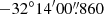 . This source shows a two-sided X-ray and radio jet during the 2003 outburst (Corbel et al. 2005). In applying a kinematic model to the trajectories of the jet, the distance to this source is found to be 8.5± 0.8 kpc, and the inclination angle of the jet is 75°±3°. The proper motion of the jet (Corbel et al. 2005) places the source at a maximum distance of 10.4± 2.9 kpc. The source has shown both high-frequency as well as low-frequency quasi-periodic oscillations (QPOs; Homan et al. 2005; Remillard et al. 2006). The presence of a high-frequency QPO gives a strong indication of a high inclination system. The spin of the black hole is constrained in the range of −0.3 < a < 0.7 (Steiner et al. 2012) from X-ray spectral modelling. Even though not much information is available about the nature of the companion star, Chaty et al. (2015) propose that the companion star is a late-type main-sequence star. The mass of the primary has not been dynamically confirmed; however, both timing as well as spectral studies reveal the black hole as a primary. Tursunov & Kološ (2018) found the mass (M) to be 11.2 M⊙ and spin to be 0.4 from the magnetic relativistic precession model to explain the twin high-frequency QPOs and low-frequency QPO. By fitting the spectrum using the two-component advective flow model and the spectral index versus QPO correlation, Molla et al. (2017) estimated the mass of the compact object to be
  . Whereas Bhattacharjee et al. (2017) constrained the mass of the black hole in the range of 10.31 M⊙ − 14.07 M⊙ from spectral modelling and the evolution of the QPO frequency. Also, Connors et al. (2019) found 9 M⊙ ≤ M ≤ 13 M⊙ using the orbital resonance model to explain high frequency QPOs.
There have been several spectral studies of the individual outbursts of the source in the literature, but a complete study of all of the outbursts in the RXTE era has not been done yet. In the present work, we present a systematic spectral analysis of all eight outbursts during the RXTE era. We start with a summary of the outburst history of H1743−322 in Sect. 2.1. We discuss the observation and data analysis in Sect. 2.2. The PCA lightcurves and HID of all outbursts are presented in Sect. 3, and we discuss the spectral characteristic in Sect. 3.1. We would like to study the evolution of accretion dynamics of the source and connect the spectral properties with the accretion parameters. Therefore, we modelled the PCA spectra using a hydrodynamical accretion flow model in Sect. 3.2 and estimate the accretion parameters for each observation (Sect. 3.3). We applied irradiated DIM in the presence of both Keplerian and sub-Keplerian component accretion flow and study the evolution of accretion parameters using a toy model in Sect. 3.4. We discuss the issues related to modelling the 2003 outburst and the related modification in Sect. 3.5, and finally, we conclude in Sect. 4.
2. Observations
2.1. Outburst history of H1743−322
After the first X-ray activity of H1743−322 was detected by Ariel 5 in 1977 (Kaluzienski & Holt 1977), the source was nearly inactive for 25 years. Though the source was detected by EXOSAT in 1984 (Reynolds et al. 1999) and by the TTM/COMIS telescope onboard the Mir-Kvant observatory in 1996 (Emelyanov et al. 2000). The International Gamma-ray Astrophysics Laboratory (INTEGRAL) detected a major outburst in March 2003, and many space-based as well as ground-based observatories carried out the follow-up observations. Using these data, extensive studies on the 2003 outburst have been carried out (Steeghs et al. 2003; Baba et al. 2003; Steiner et al. 2012; Homan et al. 2005; Remillard et al. 2006; Kalemci et al. 2006; Li et al. 2013; McClintock et al. 2009). The source has undergone multiple outbursts with a recurrence period of 0.5 to 1 year after the 2003 outburst. But the 2003 outburst was the brightest and longest outburst of H1743−322. During the RXTE era, the 2003 outburst was then followed by the 2004 (Rupen et al. 2004; Swank 2004; Bhattacharjee et al. 2017), 2005 (Swank et al. 2005; Rupen et al. 2005; Coriat et al. 2011), 2008a (Kalemci et al. 2008; Jonker et al. 2010), 2008b (Prat et al. 2009; Motta et al. 2010), 2009 (Motta et al. 2010; Chen et al. 2010; Miller-Jones et al. 2012), 2010a (Zhou et al. 2013), 2010b (Zhou et al. 2013), and 2011 (Zhou et al. 2013) outburst. Multiple outbursts are named by adding a, b after the year 2008 and 2010. The RXTE/ASM (red line) and MAXI (blue line) lightcurves of these outbursts are shown in Fig. 1 between 2003 and 2011. The RXTE/ASM lightcurve was rescaled by a factor of 1/25 to match the MAXI lightcurve.
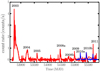 |
Fig. 1. RXTE/ASM (2−10 keV) in red colour and MAXI/GSC (2−6 keV) in blue colour represent lightcurves of H1743−322 between 2003 and 2011. The RXTE/ASM lightcurve was rescaled by a factor of 1/25. |
2.2. Observation and data analysis
In this work, we analyse all publicly available RXTE/PCA archival data between the 2003 March 28 to 2011 June 22. Table 1 provides details on the starting date, ending date, and duration of PCA observations of these outbursts. Since RXTE/PCA did not observe the rising phase of the 2004, 2008a, and 2010a outbursts, we calculated the duration of these outbursts following RXTE/ASM and MAXI/GSC lightcurves as well as Tetarenko et al. (2016). The start times of these outbursts are 2004 June 26 (MJD 53182), 2007 December 12 (MJD 54446.01), and 2009 December 15 (MJD 55180) for the 2004, 2008a, and 2010a outbursts, respectively. We do not consider the 2005 outburst in our study as very few RXTE/PCA observations are available.
Outbursts and durations.
All of the spectral studies presented in this paper are based on RXTE/PCA data. We used standard-2 (FS4a*.gz) PCA data, which have a time resolution of 16 sec for spectral analysis. The data reduction was carried out by HEASOFT software version 6.26 following the standard procedure given in the RXTE data reduction cookbook. The PCA spectra were extracted from the most stable proportional counter unit (PCU2). Using standard FTOOLS tasks, the source spectra, background spectra, and response matrix were generated. We used 3.0−45.0 keV spectra without any grouping or binning for spectral analysis. We used XSPEC version 12.10.1f for the spectral fitting of PCA data. To account for the residual uncertainties in the instrument calibration, a systematic error of 0.5% was added during spectral modelling.
3. Results and discussions
We used phenomenological models, such as powerlaw, and/or multi-colour disc blackbody (diskbb) models along with ISM absorption component (TBabs) to fit the data. Also, we used additional components, such as the absorption edge (edge) and/or the smeared absorption edge (smedge; Ebisawa et al. 1994), a Gaussian profile (gauss) in the energy range of 6−7 keV, and a high-energy cut-off (highecut) whenever required. These additional models were particularly required to fit the 2003 outburst data, whereas these additional components were only used occasionally to model the other outbursts. For a few observations in 2003, a broken powerlaw (bknpower) model was used in place of the powerlaw model. The photoelectric absorption with the abundance wilm (Wilms et al. 2000) and absorption cross section vern (Verner et al. 1996) were used for the spectral fitting. The hydrogen column density (nH) along the line of sight are quoted in the literature as 1.6 × 1022 cm−2 (Capitanio et al. 2009), 1.8 ± 0.2 × 1022 cm−2 (Prat et al. 2009), 2.2 × 1022 cm−2 (McClintock et al. 2009), and 2.3 × 1022 cm−2 (Miller et al. 2006). We fixed the nH to 1.8 × 1022 cm−2 (Prat et al. 2009) for spectral fitting. We used χ2 statistics, and the model parameters were estimated within a 90% confidence level using the migrad method. The reduced χ2 of the model fitting comes in the range of 0.7−1.4. The Gaussian line energy varies between 6.2 and 6.9 keV and the line width is in the range of 0.4−1.2 keV. We calculated the total flux in the energy range of 3.0−20.0 keV for each PCA observation of H1743−322 during the period from 2003 to 2011 and we created 3.0−20.0 keV PCA lightcurves for all the outbursts, which are shown in Fig. 2. Day zero of each outburst is given in Table 1, except for the 2004, 2008a, and 2010a outbursts (see caption of Table 1). The spectral state classification of outbursts are discussed in the literature (Chakrabarti et al. 2019; Bhattacharjee et al. 2017; Mondal et al. 2014; Debnath et al. 2013; Zhou et al. 2013; Motta et al. 2010). Here onwards, we use the same colour-coding and symbols as in Fig. 2 to represent different outbursts and their spectral states throughout the paper. Since the 2003 outburst is very bright, we rescaled the flux value by 1/6 in Fig. 2 for comparison purposes with the other outbursts. RXTE/PCA does not have coverage in the rising part of the 2004, 2008a, and 2010a outbursts, and hence we were only able to include the results from the decline part of the outbursts. The 2003 and 2004 outbursts are long-duration outbursts, whereas others have approximately a 60 day duration.
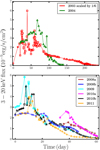 |
Fig. 2. RXTE/PCA 3.0−20.0 keV lightcurves of H1743−322 outbursts in the period 2003−2011 are drawn. The lines with different colours show different outbursts: 2003 (red); 2004 (green); 2008a (brown); 2008b (blue); 2009 (cyan); 2010a (magenta); 2010b (black); and 2011 (orange). The different symbols represent spectral states as follows: LHS (circles); HIMS (star); SIMS (square); and HSS (triangle). |
We calculated the 3−6 keV and 6−20 keV flux from spectral modelling. The ratio of the 6−20 keV flux to the 3−6 keV flux is defined as hardness. In Fig. 3, we plotted HID to provide a comparison of different outbursts. As mentioned earlier, RXTE/PCA has full coverage of the 2003, 2008b, 2009, 2010b, and 2011 outbursts, and the HID shows the complete evolution of all the spectral states, aside from 2008b. The HID of all these outbursts (other than 2008b) shows a horizontal branch where a hard to soft state transition occurs at a high flux value in the rising phase, whereas a soft to hard state transition occurs at a lower flux in the declining phase. The system shows a hysteresis pattern, similar to other transient black hole X-ray binaries (Nandi et al. 2018; Belloni et al. 2005; Muñoz-Darias et al. 2013). Whereas for the 2004, 2008a, and 2010a outbursts, the rising part in HID is missing. The 2008b outburst also shows a hysteresis nature, but it has never made a transition to HSS. Thus 2008b outburst is categorised as a failed outburst (Capitanio et al. 2009). All of the other outbursts can be classified as complete outbursts since the source has shown a transition to HSS and then back to the hard state.
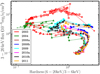 |
Fig. 3. HID of eight outbursts of H1743−322 during 2003−2011 using PCA data are shown. Each curve starts from the upper right corner (LHS) and traverses in an anti-clockwise direction, creating a hysteresis. Different colours and symbols have the same meaning as in Fig. 2. |
3.1. Evolution of spectral parameters
We estimated different spectral parameters with their uncertainties from the phenomenological spectral modelling. In Fig. 4, the evolution of the inner disc temperature (Tin) of the diskbb model is shown for the (a) 2003, (b) 2004, (c) 2008a, (d) 2008b, (e) 2009, (f) 2010a, (g) 2010b, and (h) 2011 outbursts of H1743−322. In the rising and declining part of the outbursts, the accretion disc contribution to the flux is very low and hence Tin is either small or the disc does not exist in LHS. As the outburst progresses, materials in the accretion disc get accreted to the central black hole and the disc moves inwards. Thus Tin increases and maintains roughly a constant value (either HSS or the intermediate state) for long-duration outbursts (the 2003 and 2004 outbursts) of H1743−322. Generally, Tin is higher for the 2003 outburst and reaches a maximum value of 1.6 keV on MJD 52765.836. Finally, Tin starts to decrease towards the decline part as there is not much contribution from the accretion disc. The duration of all of the other outbursts is much smaller, typically around 60 days, and the Tin evolution is quite fast. We see from Figs. 4c,d,f that the diskbb component is only required for a few observations for the 2008a, 2008b, and 2010a outbursts, respectively. The evolution of the diskbb normalisation for all of the outbursts are plotted in Fig. 5 for the (a) 2003, (b) 2004, (c) 2008a, (d) 2008b, (e) 2009, (f) 2010a (g) 2010b, and (h) 2011 outbursts. The disc norm has higher values for the 2003 and 2004 outbursts (Figs. 5a,b) and approximately remains constant with high values during the SIMS/HSS over a period of 100 days. Whereas for other outbursts, a significant change in the disc norm is observed within HSS.
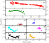 |
Fig. 4. Evolution of inner disc temperature (Tin) for the (a) 2003, (b) 2004, (c) 2008a, (d) 2008b, (e) 2009, (f) 2010a, (g) 2010b, and (h) 2011 outbursts of H1743−322. Different colours and symbols are the same as in Fig. 2. The calculated uncertainties (marked within the symbol) are within a 90% confidence range. |
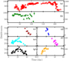 |
Fig. 5. Evolution of diskbb normalisation for the (a) 2003, (b) 2004, (c) 2008a, (d) 2008b, (e) 2009, (f) 2010a, (g) 2010b, and (h) 2011 outbursts of H1743−322. Different colours and symbols are same as in Fig. 2. The calculated uncertainties are within a 90% confidence range and marked within the symbol. |
The evolution of the photon index is shown in Fig. 6 for the (a) 2003, (b) 2004, (c) 2008a, (d) 2008b, (e) 2009, (f) 2010a, (g) 2010b, and (h) 2011 outbursts. The powerlaw component is required to model the data almost throughout the outbursts. At the beginning of the outburst, the spectrum is hard (LHS), and the photon index is ∼1.5. As the outburst progresses, the spectrum becomes softer with a photon index of ∼3 in HSS, and again it decreases towards the decline part of the outbursts. In the 2003 and 2004 outbursts, the photon index reaches close to 3, whereas for other outbursts the highest photon index is close to 2.25. Even though the rising part is missing for the 2004, 2008a, and 2010a outbursts (Figs. 6b,c,f), these outbursts still confirm the general trend of evolution. The powerlaw normalisation is plotted in Fig. 7 in the following sequence: the (a) 2003, (b) 2004, (c) 2008a, (d) 2008b, (e) 2009, (f) 2010a (g) 2010b, and (h) 2011 outbursts. For shorter duration outbursts (Figs. 7c−h), the powerlaw normalisation shows a sharp increase towards the intermediate state and HSS and then it decreases towards the decline part of the outburst. Whereas the powerlaw normalisation shows a random variation in the rising part of the 2003 outburst and stays at a constant low value after 80 days until the end of the outburst. The 2003 outburst is distinctly different from other outbursts due to the presence of a very strong powerlaw component; the highest powerlaw norm is ∼16 in comparison with ∼2 for other outbursts.
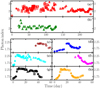 |
Fig. 6. Evolution of photon index for (a) 2003, (b) 2004, (c) 2008a, (d) 2008b, (e) 2009, (f) 2010a, (g) 2010b, and (h) 2011 outbursts of H1743−322. Different colours and symbols have their usual meaning as in Fig. 2. The calculated uncertainties (marked within the symbol) are within a 90% confidence range. |
3.2. Dynamical modelling of the outbursts
The X-ray spectrum of the black hole X-ray binary system mainly consists of two components (Mitsuda et al. 1984): a soft thermal component generated from the accretion disc and a hard powerlaw component due to the inverse-Comptonisation of soft photons that originated from the accretion disc by the high energy electron sources, including namely the Compton cloud, plasma cloud, and hot corona (Narayan & Yi 1995; Chakrabarti & Titarchuk 1995). Many models for the soft component (Shakura & Sunyaev 1973; Shimura & Takahara 1995, and reference therein) as well as Comptonisation models (Sunyaev & Titarchuk 1980, 1985; Titarchuk 1994; Lightman & Zdziarski 1987) have been proposed in the literature to explain the observed data. But these phenomenological models are not connected with the dynamics of the flow and hence they do not link the spectral parameters (discussed in Sect. 3.1) with the accretion parameters. Also, the spectral state transitions (Belloni 2010) and time delay (Smith et al. 2001, 2002, 2007) between low and high energy photons in XRBs demand a dynamic Compton corona. A two-component advective accretion flow model (Chakrabarti & Titarchuk 1995; Chakrabarti & Mandal 2006) serves all of these purposes. In this model, the Keplerian disc stays on the equatorial plane of the binary system, and a sub-Keplerian halo sandwiches the Keplerian disc from top and bottom. The Keplerian disc is static, whereas the sub-Keplerian halo component has a significantly large radial velocity. In fact, the black hole inner boundary condition demands a supersonic radial velocity near to the event horizon. In the presence of angular momentum, the supersonic sub-Keplerian flow faces a centrifugal barrier or, in extreme cases, a shock transition where the bulk kinetic energy of the flow is converted into the thermal energy due to geometric compression. Hence the centrifugal barrier or the post-shock region (PSR) serves as a reservoir for hot electrons. The Keplerian disc supplies multi-colour blackbody photons, whereas the hot electrons in the dynamic PSR inverse-Comptonise the blackbody soft photons, thus producing the hard photons. It is assumed that the Keplerian disc is truncated at the centrifugal barrier or the shock. Here, the flow properties (e.g. namely the radial velocity of the flow, number density distribution, electron and proton temperature distributions) were calculated by solving the hydrodynamic equations in the presence of radiative processes (in the present case, Compton cooling of the intercepted blackbody photons). The radiation spectrum from PSR was calculated using the hydrodynamic solutions of the sub-Keplerian halo (Mandal & Chakrabarti 2005; Chakrabarti & Mandal 2006). Finally, the resultant spectrum is a combination of both the multi-colour blackbody and the Comptonised spectrum from PSR.
The two-component advective flow model (TCAF) has already been implemented in XSPEC (Debnath et al. 2014; Iyer et al. 2015) as a table model. This model has five input parameters which are (i) the mass of the black hole M (in units of M⊙); (ii) the Keplerian accretion rate ṁd (in units of ṀEdd), where ṀEdd = 1.4 × 018(M/M⊙) gm s−1 with 10% accretion efficiency; (iii) the sub-Keplerian accretion rate ṁh (in units of ṀEdd); (iv) the size of the centrifugal barrier (PSR) xs (in units of the Schwarzschild radius  , where G is the universal gravitational constant and c is the speed of light in vacuum); and (v) the overall normalisation of the model.
We carried out the spectral modelling of the background subtracted RXTE/PCA data with the two-component model. We were able to model each observation, excluding the 2003 outburst, for which we had already done the phenomenological spectral modelling in Sect. 3.1. The rising phase of the 2003 outburst is an order of magnitude brighter than the other outbursts of the source, and we were not able to model this outburst with the two-component accretion flow model. This particular issue is addressed in Sect. 3.5. Also, we occasionally used additional model components, such as gauss, edge, or smedge, whenever required since the physical processes responsible for these model components are not included in the two-component model. We used TBabs for the absorption model with the wilms abundance table and vern (Verner et al. 1996) photoelectric absorption cross-sections. We froze the line of sight nH at 1.8 × 1022 cm−2 (Prat et al. 2009). The χ2 statistics were used for the spectral fitting. It was found that the value of reduced-χ2 varies between 0.6 to 1.4. The uncertainty in each parameter was calculated within a 90% confidence level using the migrad method. The Gaussian line energy varies between 6.2 and 6.9 keV and line width is in the range of 0.4 keV−1.2 keV. We estimated the model parameters from the spectral fitting of each observation data.
3.3. Estimation of accretion parameters of the source
The mass of the central compact object is one of the key parameters of the two-component flow model. We estimated the mass of the source for all PCA observations, which are plotted in Fig. 8 with a 90% confidence error. The 2004 outburst has a much longer duration than the other outbursts, and hence the time axis of the 2004 observations are indicated separately on the top axis. The estimated mass is consistent between outbursts and varies between 8.58 and 10.98 M⊙ for 90% of the observations. Also, a simple average mass of all the estimates with a standard deviation comes to 9.95± 0.69. Also, the scattering in the estimated mass may be due to the presence of an outflow or jet in LHS, which is not included in the model. Also, the additional model components (smedge/edge, gauss) were not consistently calculated using the two-component flow paradigm and hence this may affect the estimates. We estimated the accretion parameters (ṁd, ṁh, xs) with 90% confidence uncertainty for every PCA observation of the source during these outbursts. The time evolution of the other accretion parameters are plotted in Fig. 9 (ṁd), Fig. 10 (ṁh), and Fig. 11 (xs), respectively.
3.4. Modelling the evolution of accretion parameters
We attempt to understand the general behaviour of the evolution of accretion parameters in light of the DIM (see Lasota 2001 for a detailed review) and including irradiation (King et al. 1997) due to the activities close to the central compact object. In the two-component flow model, the accretion activity, if any, during the quiescent state is purely sub-Keplerian in nature, and the source remains faint as the sub-Keplerain flow is generally radiatively inefficient. The outburst was triggered due to the thermal-viscous instability in the Keplerian disc, and it enters into a hot state with the enhancement of viscosity, which allows matter to accrete. This increases the supply of soft photons and hence hard photons as well due to inverse Comptonisation at the PSR. The enhanced luminosity of the central region irradiates the outer part of the disc, and the entire Keplerian disc transfers into a hot phase. Since the sub-Keplerian disc sandwiches the Keplerian disc from top to bottom, the effect of irradiation at the outer part of the disc converts the sub-Keplerian matter into Keplerian matter due to enhancement of viscosity (Giri & Chakrabarti 2013). This reduces ṁh and it remains at a very low value (Fig. 10) as long as irradiation is active. During the irradiation phase, ṁd remains high (Fig. 9) above a critical disc accretion rate (ṁdc), which makes the system persistent. The effect of irradiation, as well as outburst activity, reduces when a significant fraction of matter in the Keplerian disc is being accreted by the central source. Hence, the Keplerian disc recedes outwards, and reduction of viscosity switches the Keplerian disc to a cold state. This allows the sub-Keplerain flow to rebuild. We applied irradiated DIM in the two-component flow scenario to investigate the accretion dynamics. In a previous study, Mandal & Chakrabarti (2010) used a powerlaw variation of accretion rates to model the HID of GRO J1655−40, but they did not model the observed spectra to extract the flow parameters. Whereas Lipunova (2015) show that a powerlaw variation of the Keplerian accretion rate could produce a FRED profile of outburst.
Here, we use a powerlaw model to study the evolution of accretion parameters since the outbursts of H1743−322 have a shorter (∼10 days) rise time. We assume that the accretion rates (ṁd and ṁh) vary with time as a powerlaw, whereas xs moves at a constant speed. We define the following four characteristic time scales: two timescales (th, ts) are associated with ṁh in the rising and declining phase, respectively; the other two timescales (tr, td) are linked with ṁd in the rising and declining phase, respectively. Since shock can only be present in sub-Keplerian flow, the variation of xs corresponds to the same time scale as in ṁh. The general behaviour of the time-dependent accretion rates and the shock locations are assumed as follows. The Keplerian accretion rate evolves with time as
![Mathematical equation: $$ \begin{aligned} \dot{m}_{\rm d}= {\left\{ \begin{array}{ll} A[(t_{\rm r}+1)-t]^\alpha ,&t<t_{\rm r} \\ A,&t_{\rm r} < t < t_{\rm d}\\ A[t-(t_{\rm d}-1)]^\alpha ,&t>t_{\rm d} \end{array}\right.} \end{aligned} $$](/articles/aa/full_html/2020/05/aa37577-20/aa37577-20-eq5.gif) (1)
(1)
where A is an average value of the Keplerian accretion rate in the unit of Eddington rate during a highly active phase, t is time in days, and α is a free parameter which defines the steepness of the evolution.
The sub-Keplerian accretion rate varies as
![Mathematical equation: $$ \begin{aligned} \dot{m}_{\rm h}= {\left\{ \begin{array}{ll} B[t_{\rm h}-(t-1)]^{\beta },&t<t_{\rm h}\\ B,&t_{\rm h} < t < t_{\rm s}\\ B[t-(t_{\rm s}-1)]^{\beta },&t>t_{\rm s} \end{array}\right.} \end{aligned} $$](/articles/aa/full_html/2020/05/aa37577-20/aa37577-20-eq6.gif) (2)
(2)
where B is an average minimum value of ṁh in the Eddington rate, β is a free parameter, and t is time in days.
The time variation of the shock location is assumed to be
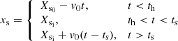 (3)
(3)
where Xs0 is the outer most value of shock location at the triggering of the outburst, v0 is the constant velocity of shock front per day, and Xsi is the inner most location of the shock.
We fitted the general trend of ṁd in Fig. 9 using Eq. (1), ṁh in Fig. 10 using Eq. (2), and xs in Fig. 11 using Eq. (3), respectively. The red solid line in Figs. 9–11 represent the model fitting to the estimated parameters, and the best fit parameters in Eqs. (1)–(3) are listed in Table 2. In the two-component model, ṁd directly regulates the soft flux, whereas ṁh responds to the hard flux. Hence, the four time scales should be related to the change in soft and hard flux during the rising and decline phase. In principle, these time scales should not be free parameters; rather, they must be estimated from the soft and hard lightcurves, given a continuous monitoring of the outburst events. We have marked these four times scales during the 2009 outburst as an example in Fig. 12. The rising time tr is associated with the first peak in the 3−6 keV lightcurve, whereas td is the time scale beyond which there is no more activity at the outer part of the Keplerian disc and the low energy flux smoothly declines. Similarly, th represents the first peak in the rising part of 6−20 keV lightcurve, and after time ts, 6−20 keV flux always remains above the 3−6 keV flux. The crossing over of the soft and hard flux takes place between td and ts. After ts, the outburst continues to decay to the quiescent state. These features in the lightcurve are very generic to all of the outbursts from the source. The best-fit values of these four-time scales (Table 2) for all outbursts closely match with the features marked in Fig. 12. We were not able to estimate tr and th for the 2004, 2008a, and 2010a outbursts since the PCA observations are not available during the rising phase of these outbursts. It is also important to note that a time-lag between th and tr is expected, and the same has been observed (Yu et al. 2004; Aneesha et al. 2019) in many outbursting sources. But it is difficult to detect this time-lag for H1743−322 as the outbursts rising time is short (∼10 days), and the closest interval between successive PCA observations are of the order of a day.
Model parameters for the evolution of ṁd, ṁh, and xs.
In Table 2, the parameter α relates to the stiffness of the rise and declination of the soft photons, whereas A is the average value of ṁd during irradiation. The parameters β and B represent the same thing for ṁh. In general β is higher than α as the former corresponds to the radiative cooling time scale whereas the later is related to the viscous time scale. Also the higher the
value of A, the brighter the outburst and B remains very low during the irradiation phase. The 2004 outburst is brighter than the other outbursts with the higher value of A and α as well as having the smallest value of B. Here, the effect of irradiation works more than 80 days (Fig. 9a) and the outburst continues for a much longer duration than the other outbursts. An extended Keplerian disc with a higher viscosity during the hot phase (Cannizzo et al. 1995; Lipunova 2015) may possibly result in a longer duration for the irradiation. The values of these parameters for other outbursts are similar, except for 2008b with the least value of A = 0.076 and α = −0.11. Also, the hard flux always dominates over the soft flux for the 2008b outburst with a very different value for th and tr than the other outbursts. In this case, the outburst never progresses to an irradiation phase (Fig. 9c), and ṁd does not cross the critical accretion rate (ṁdc) required to switch to an active phase. Table 2 shows that A = 0.087 leads to a full outburst in 2011. Hence, the 2008b outburst (marked with blue in Fig. 3) marginally failed to produce a full outburst and it allows one to constrain ṁdc for the system within a narrow range of 0.076 < ṁdc < 0.086. The orbital parameters for H1743−322 are not known and we predicted some of these values using estimated ṁdc and M values. We assume ṁdc = 0.085 and M = 10.0 and calculated an outer radius of the Keplerian disc as R0 = 2.7 × 10¹¹ (M ṁdc)1/2 = 2.5 × 1011 cm (King & Ritter 1998). Similarly, the orbital period of the system can be calculated as P = 15.07 h (Frank et al. 1992). The secondary is a late-type main-sequence star (Chaty et al. 2015) and the mass of the secondary can be estimated as 0.11 P = 1.65 (Frank et al. 1992) and hence the mass ratio of the system is q = 0.13. Also, we estimated the disc temperature and hence the sound speed at R0 using ṁdc, M and assumed the viscosity parameter αh = 0.1 in the hot state as cs = 1.2 × 106 cm s−1. The rising time of the outburst tr = R0/αhcs ∼ 25 days matches with the rising time of the 2003 outburst. Whereas all of the other complete outbursts have a 7 − 10 day rise time and hence outburst triggering must have happened at least at half of R0. Since the 2003 outburst was triggered after a very long quiescent, the system had enough time to accumulate matter and build an extended Keplerian disc. The outburst must have been triggered at R0 and the long duration of irradiation continued in the outburst for over 200 days. The 2004 outburst was possibly produced from the unused matter of 2003 (Chakrabarti et al. 2019) and could continue to produce another long outburst, but one that is much weaker than the 2003 outburst. Whereas, the outbursts between 2008 and 2011 are more frequent, fainter outbursts with a duration of ∼60 days. This may indicate that the strong irradiation in 2003 has affected the secondary in addition to push the pileup radius inside. Three prompt peaks (red points in Fig. 2), which are separated by 10−15 days, in the 2003 lightcurve reveal this interesting observation. We understand that the first peak indicates the triggering of the outburst, whereas the second and third peaks are associated with irradiation of the outer disc and secondary, respectively. The illumination due to irradiation may result in additional mass loss from the secondary (Augusteijn et al. 1993; Chen et al. 1993) and generates this kind of flickering in the lightcurve. We also see flickering, with time scale of 3−5 days, in the lightcurves of the 2009, 2010b, and 2011 outbursts. But this cannot be due to the irradiation effect on the secondary as the time scale is too short. Rather it may be due to the local instability that generated inside the disc by the competition between different radiative cooling time scales, which disturb the energy balance. Whereas Janiuk & Czerny (2011) have proposed that this small scale flickering may originate since the magnetic field works in the local dynamical scale but the magnetic cell size is of the order of the disc height.
The shock location (xs) controls the relative ratio of the soft and hard photons and hence the spectral index. The location of the shock and hence the size of the PSR changes due to the inverse-Comptonisation cooling by the soft photons from the Keplerian disc. Thus the shock moves inwards as ṁd increases and simultaneously ṁh also decreases, transiting the source into a spectrally soft state. The initial value, xs0, can be thought of as the inner edge of the Keplerian disc at the beginning of the outburst. We were not able to quote its value for the 2004, 2008a, and 2010a outburst as the rising phase data are not available. The closest value of the shock location generally remains ∼10 rg during HSS but it can reach close to ∼5 rg as well. We assumed a constant shock speed, which is sufficient for the present work but in general it may be in accelerating motion (Chatterjee et al. 2016; Nandi et al. 2018) as well. The values of the parameters in Table 2 fit the general profile of the accretion parameters (Figs. 9–11) and the quoted values were estimated manually by minimising χ2. Since this is a manual fitting, we were not able to estimate the error in the parameters and this is one of the caveats in the present work.
3.5. Modelling the 2003 outburst
The 2003 outburst of H1743−322 is very bright and has a long duration, which is different from other outbursts of the source. We tried to fit the outburst data using the two-component flow model and understood that it is not possible to model the entire outburst using the accretion disc model alone. To illustrate the situation better, we used the phenomenological model fitting results described in Sect. 3.1 of the outbursts having full PCA coverage. We would like to understand the relative contribution of the blackbody and powerlaw component and hence only used the observations that can be modelled by diskbb+powerlaw. The powerlaw photon flux between energy E1 and E2 can be calculated as 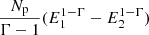 , where Np is the powerlaw normalisation and Γ is the photon index. Similarly, the total blackbody photon flux can be estimated as
 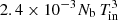 , where Nb and Tin represent the diskbb norm and inner disc temperature of the Keplerian disc. In Fig. 13, we plotted the 3−20 keV blackbody photon flux versus the powerlaw photon flux for the 2003 (red), 2009 (cyan), 2010b (black), and 2011 (orange) outbursts. We divided the entire plot into four regions (I, II, III, and IV). All of the observations in region I can be modelled using the existing version of the two-component flow model, and hence we could model all of the outbursts except for the 2003 outburst. In the two-component model, we calculated the blackbody spectrum using the effective temperature (Teff) of the accretion disc. But at a higher accretion rate ṁd, the spectrum calculation needs to be modified by the colour temperature Tc = ξ Teff (Shimura & Takahara 1995), where ξ is the hardening factor. The high value of the disc flux in region II corresponds to a high accretion rate and therefore, the disc blackbody spectrum needs to be calculated using Tc to model the observations in region II. If the high energy photons are solely produced by the inverse Comptonisation of the blackbody photons, then the observations in region IV require inverse Comptonisation of more than 50% of the blackbody photons. It is very unlikely that such a high fraction of blackbody photons are going to intercept the PSR. Also, there are more non-thermal photons than disc blackbody photons for a few observations in region IV. This indicates the requirement of an additional source of non-thermal photons to explain the observations in region IV along with the two-component model. In fact, this should be true for any physical model, and it shows the difference between a phenomenological model and a physical model. In the phenomenological model, all of the components are independent, and hence it does not justify that given a blackbody temperature, the observed spectral index and number of high energy photons can be created or not. In region III, the two-component model needs to be modified using the colour temperature as well as an additional source of non-thermal photons, which are required to model the data. Hence, we were not able to model the observations in regions II−IV. To illustrate the above picture, we modelled the observation on MJD 52765.836, which corresponds to the highest flux in the 2003 outburst and is marked by an ellipse in Fig. 13. We modified the two-component model source code to incorporate the colour temperature and we fitted the data by running the source code manually. Also, we used a powerlaw component as an additional source of non-thermal photons and the fitted result is shown in Fig. 14. The model fitted parameters are M = 10.0± 0.13, ṁd = 1.698 ± 0.034, ṁh = 0.152 ± 0.014, xs = 6.58± 0.03, ξ = 2.96± 0.01, and the photon index is Γ = 2.28± 0.01 with fitted reduced χ2 = 0.89. The estimated X-ray flux under the powerlaw component is 2.5 × 10⁻⁸ erg cm−2 s−1.
We propose that the additional powerlaw component originated from the jet. The presence of shock close to base of the jet (Vyas & Chattopadhyay 2017) may produce non-thermal electrons. We checked if the same can be produced due to synchrotron emission from non-thermal electrons at the base of the jet. We assume that 10% (Kumar & Chattopadhyay 2013) of the accreted matter is being throne as a jet. We calculated the density of material in the jet as ρ = ṁj/Ωvx2, where ṁj is the mass outflow rate, Ω = 2π(1 − cos θ), θ is the opening angle of the jet, and v = x−1/2. Here the radial distance (x) and flow speed (v) are expressed in the unit of rg and the speed of light (c). Using the mass and accretion rate from X-ray spectral modelling, θ = 30°, x = 20, we calculated the number density of electrons as 7.5 × 1016 cm−3 and an equipartition magnetic field 7.5 × 10⁶ G. The X-ray photon index corresponds to a non-thermal electron distribution of the index p = 3.48. The emitted synchrotron luminosity in 3−20 keV is 7.9 × 1038 erg s−1 (Rybicki & Lightman 1979). Assuming a distance of 8.5 kpc and an inclination angle of 75°, the estimated flux is 2.4 × 10⁻⁸ erg cm−2 s−1, which is close to the observed value. Also, we find radio observations (McClintock et al. 2009) at 4.86 GHz and 8.46 GHz, which are 10 h before and 1.7 days after the PCA observation. The reported radio fluxes are 13.78 mJy and 11.12 mJy before the PCA observation, respectively, whereas the radio fluxes are 25.62 mJy and 23.02 mJy after the PCA observation, respectively. Using the observed radio flux Sν at the frequency ν, we estimated the observed kinetic jet power (Longair 2011; Nandi et al. 2018) to be
 (4)
(4)
where f(γ, i) (Fender 2001) represents the Doppler boosting factor for the bulk Lorentz factor γ and the inclination angle (i). The other factors Δt and D are the rise time of jet and the distance to the source, respectively. For an assumed γ = 2 (mildly relativistic jet) and i = 75°, we calculated f(γ, i) = 7.47. We took Δt = 24 h and D = 8.5 kpc, and by using the observed radio flux (25.62 mJy at 4.86 GHz) we estimated the jet kinetic power as 6.5 × 1037 erg s−1. This can easily be produced by the available jet energy budget ηjṁj c2 = 6.9 × 1037 erg s−1 with ηj = 3%. The consistency of the X-ray and radio observations with typical values of outflow parameters support the jet origin of the non-thermal contribution. Also, the 2003 outburst has shown continuous radio activity throughout the outburst even in SIMS and HSS, meaning that there is a significant non-thermal contribution in the X-ray spectrum. Hence, a combined accretion disc-jet model applied to both X-ray and radio observations are required to better understand the 2003 outburst, which we aim to attempt in the future.
We tried to connect the accretion dynamics to the ejection of a jet using radio observations of outbursts other than the 2003 outburst. We find good radio coverage for the 2009 outburst (Miller-Jones et al. 2012). To understand the radio and X-ray connection, in Fig. 15 we plotted the radio lightcurve along with the model fitted ṁd and ṁh for the X-ray observations within a day before the radio observation. The radio observations are available only in HIMS (star) and HSS (triangle). In the rising phase of the outburst, a steady radio flux is observed in HIMS with low ṁd and a significant hard X-ray flux. The steady radio flux is possibly associated with a compact jet and indicates the coupling of the accretion disc, PSR with the compact jet. In fact, the Very Large Baseline Array (VLBA) images (Miller-Jones et al. 2012) of the source at 8.4 GHz clearly shown the presence of an unresolved compact jet during this period (MJD 54979.35, 54981.35, and 54984.35). Whereas a transient jet is observed in the VLBA images on MJD 54987.33 and MJD 54988.33. This corresponds to the highest radio flux in Fig. 15 at the beginning of the HSS, which is a characteristic of a spectral state transition from HIMS/SIMS to HSS observed in many outbursting sources (Brocksopp et al. 2005; Corbel et al. 2004). This transient radio activity is associated with an increase of ṁd and a sharp decrease of ṁh. The radio flux density decreases sharply in the HSS and remains at a very low level. This is due to the quenching of a jet since a high ṁd can completely cool the PSR with a very small ṁh. Towards the end of HSS state, the radio flux starts increasing, which represents the reappearance of a compact jet due to an increase of ṁh in the presence of PSR, and it reaches a steady value towards the decline part of the outburst.
4. Conclusions
The 2003 and 2004 outburst lightcurves (Fig. 2) have a long duration whereas others have a duration of ∼60 days with a regular recurrence period of 7 − 9 months (Table 1). Like other outbursting XRBs, this source also shows a canonical HID pattern (Fig. 3) and spectral state transitions during outbursts. The 2003 and 2004 outbursts are more luminous and have reached a much softer state (hardness ratio ∼0.15) in comparison to other outbursts (hardness ratio ∼0.4). In this work, we present both the spectral as well as dynamical evolution of outbursts of H1743−322 using RXTE/PCA data. We see from the spectral fitting (Figs. 4 and 5) that in the LHS (both beginning and end) of outbursts, the diskbb component is not present (or very small), whereas the powerlaw component (Fig. 6) is hard (Γ ∼ 1.5). This can be understood from the combined role of accretion parameters. During LHS, ṁd is low (Fig. 9), the inner edge of the disc xs (Fig. 11) is further apart, and hence there are not as many soft photons. Whereas ṁh is high, and hence electrons in the PSR are hot. The net result is a hard spectrum due to strong inverse-Comptonisation by PSR. As the outburst progress towards intermediate states, Tin increases, and diskbb norm (Fig. 5) is at its maximum in the HSS, except for 2008b where the diskbb norm is much lower and the outburst never progresses to HSS. The source luminosity increases, and the spectrum becomes softer as Γ increases along with the increase of powerlaw norm (Fig. 7). This is supported by the increase of ṁd (Fig. 9) and decrease of xs (Fig. 11), which increase the supply of soft photons, whereas decreases in ṁh (Fig. 10) and the size of PSR (xs) reduce the supply of hot electrons. This enhances the cooling of PSR, producing a softer spectrum. In HSS of the 2003 and 2004 outbursts, the photon index reaches ∼3, whereas other outburst spectra are relatively harder. During the decline phase, the behaviour of the accretion parameters are the reverse.
 |
Fig. 7. Evolution of powerlaw normalisation for the (a) 2003, (b) 2004, (c) 2008a, (d) 2008b, (e) 2009, (f) 2010a, (g) 2010b, and (h) 2011 outbursts of H1743−322. Different colours and symbols have the same meaning as in Fig. 2. The 90% uncertainty of the parameter is marked within the symbol. |
 |
Fig. 8. Mass of the source estimated from two-component flow model for different outbursts are plotted. Different colours and symbols have the same meaning as in Fig. 2. The uncertainty in mass is quoted within the 90% confidence range and is marked within the symbols. The time axis on top is applicable to only the 2004 outburst (green points). |
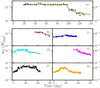 |
Fig. 9. Evolution of Keplerian disc accretion rate for the (a) 2004, (b) 2008a, (c) 2008b, (d) 2009, (e) 2010a, (f) 2010b, and (g) 2011 outbursts of H1743−322. The red solid line represents model fitting using Eq. (1). Different colours and symbols have the same meaning as in Fig. 2. The calculated uncertainties (marked within the symbol) are in the 90% confidence range. |
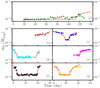 |
Fig. 10. Evolution of sub-Keplerian accretion rate for the (a) 2004, (b) 2008a, (c) 2008b, (d) 2009, (e) 2010a, (f) 2010b, and (g) 2011 outbursts of H1743−322. The red solid line represents model fitting using Eq. (2). Different colours and symbols have the same meaning as in Fig. 2. We marked the 90% uncertainty of the parameter within the symbol. |
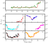 |
Fig. 11. Evolution of shock location for the (a) 2004, (b) 2008a, (c) 2008b, (d) 2009, (e) 2010a, (f) 2010b, and (g) 2011 outbursts of H1743−322. The red solid line represents model fitting using Eq. (3). Different colours and symbols have the same meaning as in Fig. 2. The 90% confidence uncertainties are marked within the symbol. |
The mass of the central object is one of the parameters in the hydrodynamic model, and we estimated the mass of the source (Fig. 8) for all of the observations which remain within 8.58 − 10.98 M⊙ for 90% of the observations. We applied irradiated DIM into the two-component flow model and used a powerlaw variation of accretion rates (Eqs. (1) and (2)) with constant motion of xs to understand the evolution of the accretion parameters. We fitted the observed data (red line in Figs. 9–11) by the proposed toy model and listed the parameters in Table 2. We identified the rise and decline timescale of ṁd (tr, td) and ṁh (th, ts) in the 3 − 6 keV and 6 − 20 keV lightcurves (Fig. 12) of the outbursts. In principle, these time scales can be determined from the lightcurves, given continuous monitoring of the outburst events. We see from Table 2 that the parameter β is higher than α as the sub-Keplerian flow responds faster than the Keplerian flow. Also, the higher the value of A, the brighter the outburst is. During irradiation, ṁd is high and there are changes around A, whereas ṁh remains at a low value. Also a closer Keplerian disc (xsi) makes the central region luminous. After the end of the irradiation phase, the Keplerian disc recedes, and the sub-Keplerain flow starts to build. The 2008b outburst has the least A = 0.076 and α = −0.11; additionally, a high energy flux always dominates the soft flux. This outburst never reaches HSS, and this is classified as a failed outburst. But the 2011 outburst has A = 0.086, and it is a full outburst. Hence the 2008b and 2011 outbursts offer an excellent opportunity to constrain the critical accretion rate 0.076 < ṁdc < 0.086 of the system. Using the estimated mass and critical accretion rate, we have commented on the orbital parameters of the system. Also, we calculated the rise time of the outburst for this system as tr = 25 days, which is the rise time of the 2003 outburst, whereas other outbursts have an approximate 10 day rise time. This indicates that the strong irradiation phase of the 2003 outburst may have pushed the pileup radius inside. All of the outbursts from 2008 onwards have a similar rise time, duration, and recurrence period, which indicate the fixed location of the pileup radius with a regular mass supply from the secondary. We associate the three distinct peaks in the 2003 outburst lightcurve to be due to the triggering of the outburst, irradiation of the cold outer disc, and irradiation of the secondary, respectively.
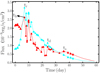 |
Fig. 12. 3−6 keV (cyan line) and 6−20 keV (red line) lightcurves of the 2009 outburst are shown. Different accretion time scales (see text for details) are marked in the observed lightcurves. |
We have discussed the issues related to modelling the 2003 outburst using the two-component model in Sect. 3.5. We plotted the powerlaw versus the blackbody contribution (Fig. 13) required to model the data. It was difficult to model the spectra in regions III and IV by an accretion disc alone due to the presence of large non-thermal components even in SIMS/HSS state. We have argued that region (II) needs a modification of effective disc temperature by colour temperature, and region IV needs an additional non-thermal contribution, whereas region III needs both of the modifications. As an example, we fitted the observation with the highest flux (in SIMS) in the 2003 outburst with these modifications, which are presented in Fig. 14. We have shown that the additional non-thermal component requires fitting data, which can be produced from the base of the jet with reasonable parameters. Also, this is consistent with the radio flux observed after this observation. So, a dynamical model coupling the disc-jet is required to fit the 2003 outburst data, which we aim to attempt in the future. Finally, we could connect the evolution of accretion dynamics with the jet launching by using radio observations in 2009 with the X-ray data. In Fig. 15, we see steady jet and radio emission at the beginning and end of the outburst due to the high contribution of ṁh and the absence (or very small contribution) of jet in the HSS due to the cooling of PSR by the high rate of accretion of Keplerian matter.
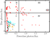 |
Fig. 13. Blackbody photon flux and the powerlaw photon flux required to model the data when both components are present. The outburst data with full PCA coverage are plotted as: 2003 (red), 2009 (cyan), 2010b (black), and 2011 (orange). The different regions (I−IV) represent the validity of the current model and possible modifications (see text for details). The data point marked by a small ellipse corresponds to the highest peak of the 2003 outburst and was modelled by the modified two-component model (see Fig. 14). |
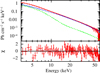 |
Fig. 14. Modelling of the 2003 outburst data (red) on MJD 52765.836 using the two-component model (green) with an additional powerlaw (blue). See text for parameters and detail descriptions. |
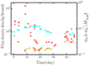 |
Fig. 15. Evolution of radio flux density (red) along with the Keplerian disc accretion rate (cyan) and sub-Keplerian accretion rate (gold) are presented for the 2009 outburst. The symbols in red represent the radio flux density at 1.4 GHz (plus), 4.9 GHz (cross), and 8.4 GHz (pentagon), respectively. The 3σ upper limit of the 1.4 GHz radio data on MJD 54996.2 is indicated by a downward arrow. The accretion rates in different spectral states are denoted by the same symbols (triangle for HSS and star for HIMS) throughout the paper. The left vertical axis represents the radio flux density, whereas the right vertical axis shows the accretion rates. |
References
- Aneesha, U., Mandal, S., & Sreehari, H. 2019, MNRAS, 486, 2705 [NASA ADS] [CrossRef] [Google Scholar]
- Augusteijn, T., Kuulkers, E., & Shaham, J. 1993, A&A, 279, L13 [NASA ADS] [Google Scholar]
- Baba, D., Nagata, T., Iwata, I., Kato, T., & Yamaoka, H. 2003, IAU Circ., 8112, 2 [NASA ADS] [Google Scholar]
- Belloni, T. 2010, The Jet Paradigm (Berlin, Heidelberg: Springer-Verlag), 794 [Google Scholar]
- Belloni, T., Homan, J., Casella, P., et al. 2005, A&A, 440, 207 [NASA ADS] [CrossRef] [EDP Sciences] [Google Scholar]
- Bhattacharjee, A., Banerjee, I., Banerjee, A., Debnath, D., & Chakrabarti, S. K. 2017, MNRAS, 466, 1372 [NASA ADS] [CrossRef] [Google Scholar]
- Brocksopp, C., Corbel, S., Fender, R. P., et al. 2005, MNRAS, 356, 125 [NASA ADS] [CrossRef] [Google Scholar]
- Cannizzo, J. K., Chen, W., & Livio, M. 1995, ApJ, 454, 880 [NASA ADS] [CrossRef] [Google Scholar]
- Capitanio, F., Belloni, T., Del Santo, M., & Ubertini, P. 2009, MNRAS, 398, 1194 [NASA ADS] [CrossRef] [Google Scholar]
- Chakrabarti, S. K., & Mandal, S. 2006, ApJ, 642, L49 [NASA ADS] [CrossRef] [Google Scholar]
- Chakrabarti, S., & Titarchuk, L. G. 1995, ApJ, 455, 623 [NASA ADS] [CrossRef] [Google Scholar]
- Chakrabarti, S. K., Debnath, D., & Nagarkoti, S. 2019, Adv. Space Res., 63, 3749 [NASA ADS] [CrossRef] [Google Scholar]
- Chatterjee, D., Debnath, D., Chakrabarti, S. K., Mondal, S., & Jana, A. 2016, ApJ, 827, 88 [NASA ADS] [CrossRef] [Google Scholar]
- Chaty, S., Muñoz Arjonilla, A. J., & Dubus, G. 2015, A&A, 577, A101 [Google Scholar]
- Chen, W., Livio, M., & Gehrels, N. 1993, ApJ, 408, L5 [NASA ADS] [CrossRef] [Google Scholar]
- Chen, Y. P., Zhang, S., Torres, D. F., et al. 2010, A&A, 522, A99 [NASA ADS] [CrossRef] [EDP Sciences] [Google Scholar]
- Connors, R. M. T., van Eijnatten, D., Markoff, S., et al. 2019, MNRAS, 485, 3696 [NASA ADS] [CrossRef] [Google Scholar]
- Corbel, S., Fender, R. P., Tomsick, J. A., Tzioumis, A. K., & Tingay, S. 2004, ApJ, 617, 1272 [NASA ADS] [CrossRef] [Google Scholar]
- Corbel, S., Kaaret, P., Fender, R. P., et al. 2005, ApJ, 632, 504 [NASA ADS] [CrossRef] [Google Scholar]
- Coriat, M., Corbel, S., Prat, L., et al. 2011, MNRAS, 414, 677 [NASA ADS] [CrossRef] [Google Scholar]
- Debnath, D., Chakrabarti, S. K., & Nandi, A. 2013, Adv. Space Res., 52, 2143 [NASA ADS] [CrossRef] [Google Scholar]
- Debnath, D., Chakrabarti, S. K., & Mondal, S. 2014, MNRAS, 440, L121 [NASA ADS] [CrossRef] [Google Scholar]
- Ebisawa, K., Ogawa, M., Aoki, T., et al. 1994, PASJ, 46, 375 [NASA ADS] [Google Scholar]
- Emelyanov, A. N., Aleksandrovich, N. L., & Sunyaev, R. A. 2000, Astron. Lett., 26, 297 [NASA ADS] [CrossRef] [Google Scholar]
- Fender, R. P. 2001, MNRAS, 322, 31 [NASA ADS] [CrossRef] [Google Scholar]
- Frank, J., King, A. R., Raine, D. J., & Shaham, J. 1986, Phys. Today, 39, 124 [CrossRef] [Google Scholar]
- Frank, J., King, A., & Raine, D. 1992, Accretion Power in Astrophysics, 21 [Google Scholar]
- Giri, K., & Chakrabarti, S. K. 2013, MNRAS, 430, 2836 [NASA ADS] [CrossRef] [Google Scholar]
- Homan, J., & Belloni, T. 2005, Ap&SS, 300, 107 [NASA ADS] [CrossRef] [Google Scholar]
- Homan, J., Miller, J. M., Wijnands, R., et al. 2005, ApJ, 623, 383 [NASA ADS] [CrossRef] [Google Scholar]
- Hōshi, R. 1979, Prog. Theor. Phys., 61, 1307 [NASA ADS] [CrossRef] [Google Scholar]
- Iyer, N., Nandi, A., & Mandal, S. 2015, ApJ, 807, 108 [NASA ADS] [CrossRef] [Google Scholar]
- Janiuk, A., & Czerny, B. 2011, MNRAS, 414, 2186 [Google Scholar]
- Jonker, P. G., Miller-Jones, J., Homan, J., et al. 2010, MNRAS, 401, 1255 [NASA ADS] [CrossRef] [Google Scholar]
- Kalemci, E., Tomsick, J. A., Rothschild, R. E., et al. 2006, ApJ, 639, 340 [NASA ADS] [CrossRef] [Google Scholar]
- Kalemci, E., Tomsick, J. A., Corbel, S., & Tzioumis, T. 2008, ATel, 1378, 1 [NASA ADS] [Google Scholar]
- Kaluzienski, L. J., & Holt, S. S. 1977, IAU Circ., 3099, 3 [NASA ADS] [Google Scholar]
- King, A. R., & Ritter, H. 1998, MNRAS, 293, L42 [NASA ADS] [CrossRef] [Google Scholar]
- King, A. R., Kolb, U., & Szuszkiewicz, E. 1997, ApJ, 488, 89 [NASA ADS] [CrossRef] [Google Scholar]
- Kumar, R., & Chattopadhyay, I. 2013, MNRAS, 430, 386 [NASA ADS] [CrossRef] [Google Scholar]
- Lasota, J.-P. 2001, New Astron. Rev., 45, 449 [NASA ADS] [CrossRef] [Google Scholar]
- Li, Z. B., Zhang, S., Qu, J. L., et al. 2013, MNRAS, 433, 412 [NASA ADS] [CrossRef] [Google Scholar]
- Lightman, A. P., & Zdziarski, A. A. 1987, ApJ, 319, 643 [NASA ADS] [CrossRef] [Google Scholar]
- Lipunova, G. V. 2015, ApJ, 804, 87 [NASA ADS] [CrossRef] [Google Scholar]
- Longair, M. S. 2011, High Energy Astrophysics (Cambridge: Cambridge University Press) [Google Scholar]
- Lutovinov, A., Revnivtsev, M., Molkov, S., & Sunyaev, R. 2005, A&A, 430, 997 [NASA ADS] [CrossRef] [EDP Sciences] [Google Scholar]
- Mandal, S., & Chakrabarti, S. K. 2005, A&A, 434, 839 [NASA ADS] [CrossRef] [EDP Sciences] [Google Scholar]
- Mandal, S., & Chakrabarti, S. K. 2010, ApJ, 710, L147 [NASA ADS] [CrossRef] [Google Scholar]
- McClintock, J. E., & Remillard, R. A. 2006, in Black Hole Binaries, eds. W. H. G. Lewin, & M. van der Klis, 157 [Google Scholar]
- McClintock, J. E., Remillard, R. A., Rupen, M. P., et al. 2009, ApJ, 698, 1398 [NASA ADS] [CrossRef] [Google Scholar]
- Miller, J. M., Raymond, J., Homan, J., et al. 2006, ApJ, 646, 394 [NASA ADS] [CrossRef] [Google Scholar]
- Miller-Jones, J. C. A., Sivakoff, G. R., Altamirano, D., et al. 2012, MNRAS, 421, 468 [NASA ADS] [Google Scholar]
- Mitsuda, K., Inoue, H., Koyama, K., et al. 1984, PASJ, 36, 741 [NASA ADS] [Google Scholar]
- Molla, A. A., Chakrabarti, S. K., Debnath, D., & Mondal, S. 2017, ApJ, 834, 88 [NASA ADS] [CrossRef] [Google Scholar]
- Mondal, S. 2020, Adv. Space Res., 65, 693 [NASA ADS] [CrossRef] [Google Scholar]
- Mondal, S., Debnath, D., & Chakrabarti, S. K. 2014, ApJ, 786, 4 [NASA ADS] [CrossRef] [Google Scholar]
- Motta, S., Muñoz-Darias, T., & Belloni, T. 2010, MNRAS, 408, 1796 [NASA ADS] [CrossRef] [Google Scholar]
- Muñoz-Darias, T., Coriat, M., Plant, D. S., et al. 2013, MNRAS, 432, 1330 [NASA ADS] [CrossRef] [Google Scholar]
- Nandi, A., Mandal, S., Sreehari, H., et al. 2018, Ap&SS, 363, 90 [NASA ADS] [CrossRef] [Google Scholar]
- Narayan, R., & Yi, I. 1995, ApJ, 452, 710 [NASA ADS] [CrossRef] [Google Scholar]
- Prat, L., Rodriguez, J., Cadolle Bel, M., et al. 2009, A&A, 494, L21 [NASA ADS] [CrossRef] [EDP Sciences] [Google Scholar]
- Remillard, R. A., McClintock, J. E., Orosz, J. A., & Levine, A. M. 2006, ApJ, 637, 1002 [NASA ADS] [CrossRef] [Google Scholar]
- Reynolds, A. P., Parmar, A. N., Hakala, P. J., et al. 1999, A&AS, 134, 287 [NASA ADS] [CrossRef] [EDP Sciences] [Google Scholar]
- Rupen, M. P., Mioduszewski, A. J., & Dhawan, V. D. 2004, Am. Astron. Soc. Meet. Abstr., 204, 05.16 [Google Scholar]
- Rupen, M. P., Mioduszewski, A. J., & Dhawan, V. 2005, ATel, 490, 1 [NASA ADS] [Google Scholar]
- Rybicki, G. B., & Lightman, A. P. 1979, Radiative Processes in Astrophysics (New York: Wiley) [Google Scholar]
- Shakura, N. I., & Sunyaev, R. A. 1973, A&A, 500, 33 [NASA ADS] [Google Scholar]
- Shimura, T., & Takahara, F. 1995, ApJ, 445, 780 [NASA ADS] [CrossRef] [Google Scholar]
- Smak, J. 1982, Acta Astron., 32, 199 [NASA ADS] [Google Scholar]
- Smith, D. M., Heindl, W. A., Markwardt, C. B., & Swank, J. H. 2001, ApJ, 554, L41 [NASA ADS] [CrossRef] [Google Scholar]
- Smith, D. M., Heindl, W. A., & Swank, J. H. 2002, ApJ, 569, 362 [NASA ADS] [CrossRef] [Google Scholar]
- Smith, D. M., Dawson, D. M., & Swank, J. H. 2007, ApJ, 669, 1138 [NASA ADS] [CrossRef] [Google Scholar]
- Steeghs, D., Miller, J. M., Kaplan, D., & Rupen, M. 2003, ATel, 146, 1 [NASA ADS] [Google Scholar]
- Steiner, J. F., McClintock, J. E., & Reid, M. J. 2012, ApJ, 745, L7 [NASA ADS] [CrossRef] [Google Scholar]
- Sunyaev, R. A., & Titarchuk, L. G. 1980, A&A, 86, 121 [NASA ADS] [Google Scholar]
- Sunyaev, R. A., & Titarchuk, L. G. 1985, A&A, 143, 374 [NASA ADS] [Google Scholar]
- Swank, J. 2004, ATel, 301, 1 [NASA ADS] [Google Scholar]
- Swank, J. H., Remillard, R., & Markwardt, C. B. 2005, ATel, 576, 1 [NASA ADS] [Google Scholar]
- Tetarenko, B. E., Sivakoff, G. R., Heinke, C. O., & Gladstone, J. C. 2016, ApJS, 222, 15 [NASA ADS] [CrossRef] [Google Scholar]
- Tetarenko, B. E., Dubus, G., Lasota, J. P., Heinke, C. O., & Sivakoff, G. R. 2018a, MNRAS, 480, 2 [NASA ADS] [CrossRef] [Google Scholar]
- Tetarenko, B. E., Lasota, J. P., Heinke, C. O., Dubus, G., & Sivakoff, G. R. 2018b, Nature, 554, 69 [NASA ADS] [CrossRef] [Google Scholar]
- Titarchuk, L. 1994, ApJ, 434, 570 [NASA ADS] [CrossRef] [Google Scholar]
- Tursunov, A. A., & Kološ, M. 2018, Phys. At. Nucl., 81, 279 [CrossRef] [Google Scholar]
- Verner, D. A., Ferland, G. J., Korista, K. T., & Yakovlev, D. G. 1996, ApJ, 465, 487 [NASA ADS] [CrossRef] [Google Scholar]
- Vyas, M. K., & Chattopadhyay, I. 2017, MNRAS, 469, 3270 [NASA ADS] [CrossRef] [Google Scholar]
- Wilms, J., Allen, A., & McCray, R. 2000, ApJ, 542, 914 [NASA ADS] [CrossRef] [Google Scholar]
- Yu, W., van der Klis, M., & Fender, R. 2004, ApJ, 611, L121 [NASA ADS] [CrossRef] [Google Scholar]
- Zhou, J. N., Liu, Q. Z., Chen, Y. P., et al. 2013, MNRAS, 431, 2285 [NASA ADS] [CrossRef] [Google Scholar]
All Tables
All Figures
|
Fig. 1. RXTE/ASM (2−10 keV) in red colour and MAXI/GSC (2−6 keV) in blue colour represent lightcurves of H1743−322 between 2003 and 2011. The RXTE/ASM lightcurve was rescaled by a factor of 1/25. |
| In the text | |
|
Fig. 2. RXTE/PCA 3.0−20.0 keV lightcurves of H1743−322 outbursts in the period 2003−2011 are drawn. The lines with different colours show different outbursts: 2003 (red); 2004 (green); 2008a (brown); 2008b (blue); 2009 (cyan); 2010a (magenta); 2010b (black); and 2011 (orange). The different symbols represent spectral states as follows: LHS (circles); HIMS (star); SIMS (square); and HSS (triangle). |
| In the text | |
|
Fig. 3. HID of eight outbursts of H1743−322 during 2003−2011 using PCA data are shown. Each curve starts from the upper right corner (LHS) and traverses in an anti-clockwise direction, creating a hysteresis. Different colours and symbols have the same meaning as in Fig. 2. |
| In the text | |
|
Fig. 4. Evolution of inner disc temperature (Tin) for the (a) 2003, (b) 2004, (c) 2008a, (d) 2008b, (e) 2009, (f) 2010a, (g) 2010b, and (h) 2011 outbursts of H1743−322. Different colours and symbols are the same as in Fig. 2. The calculated uncertainties (marked within the symbol) are within a 90% confidence range. |
| In the text | |
|
Fig. 5. Evolution of diskbb normalisation for the (a) 2003, (b) 2004, (c) 2008a, (d) 2008b, (e) 2009, (f) 2010a, (g) 2010b, and (h) 2011 outbursts of H1743−322. Different colours and symbols are same as in Fig. 2. The calculated uncertainties are within a 90% confidence range and marked within the symbol. |
| In the text | |
|
Fig. 6. Evolution of photon index for (a) 2003, (b) 2004, (c) 2008a, (d) 2008b, (e) 2009, (f) 2010a, (g) 2010b, and (h) 2011 outbursts of H1743−322. Different colours and symbols have their usual meaning as in Fig. 2. The calculated uncertainties (marked within the symbol) are within a 90% confidence range. |
| In the text | |
|
Fig. 7. Evolution of powerlaw normalisation for the (a) 2003, (b) 2004, (c) 2008a, (d) 2008b, (e) 2009, (f) 2010a, (g) 2010b, and (h) 2011 outbursts of H1743−322. Different colours and symbols have the same meaning as in Fig. 2. The 90% uncertainty of the parameter is marked within the symbol. |
| In the text | |
|
Fig. 8. Mass of the source estimated from two-component flow model for different outbursts are plotted. Different colours and symbols have the same meaning as in Fig. 2. The uncertainty in mass is quoted within the 90% confidence range and is marked within the symbols. The time axis on top is applicable to only the 2004 outburst (green points). |
| In the text | |
|
Fig. 9. Evolution of Keplerian disc accretion rate for the (a) 2004, (b) 2008a, (c) 2008b, (d) 2009, (e) 2010a, (f) 2010b, and (g) 2011 outbursts of H1743−322. The red solid line represents model fitting using Eq. (1). Different colours and symbols have the same meaning as in Fig. 2. The calculated uncertainties (marked within the symbol) are in the 90% confidence range. |
| In the text | |
|
Fig. 10. Evolution of sub-Keplerian accretion rate for the (a) 2004, (b) 2008a, (c) 2008b, (d) 2009, (e) 2010a, (f) 2010b, and (g) 2011 outbursts of H1743−322. The red solid line represents model fitting using Eq. (2). Different colours and symbols have the same meaning as in Fig. 2. We marked the 90% uncertainty of the parameter within the symbol. |
| In the text | |
|
Fig. 11. Evolution of shock location for the (a) 2004, (b) 2008a, (c) 2008b, (d) 2009, (e) 2010a, (f) 2010b, and (g) 2011 outbursts of H1743−322. The red solid line represents model fitting using Eq. (3). Different colours and symbols have the same meaning as in Fig. 2. The 90% confidence uncertainties are marked within the symbol. |
| In the text | |
|
Fig. 12. 3−6 keV (cyan line) and 6−20 keV (red line) lightcurves of the 2009 outburst are shown. Different accretion time scales (see text for details) are marked in the observed lightcurves. |
| In the text | |
|
Fig. 13. Blackbody photon flux and the powerlaw photon flux required to model the data when both components are present. The outburst data with full PCA coverage are plotted as: 2003 (red), 2009 (cyan), 2010b (black), and 2011 (orange). The different regions (I−IV) represent the validity of the current model and possible modifications (see text for details). The data point marked by a small ellipse corresponds to the highest peak of the 2003 outburst and was modelled by the modified two-component model (see Fig. 14). |
| In the text | |
|
Fig. 14. Modelling of the 2003 outburst data (red) on MJD 52765.836 using the two-component model (green) with an additional powerlaw (blue). See text for parameters and detail descriptions. |
| In the text | |
|
Fig. 15. Evolution of radio flux density (red) along with the Keplerian disc accretion rate (cyan) and sub-Keplerian accretion rate (gold) are presented for the 2009 outburst. The symbols in red represent the radio flux density at 1.4 GHz (plus), 4.9 GHz (cross), and 8.4 GHz (pentagon), respectively. The 3σ upper limit of the 1.4 GHz radio data on MJD 54996.2 is indicated by a downward arrow. The accretion rates in different spectral states are denoted by the same symbols (triangle for HSS and star for HIMS) throughout the paper. The left vertical axis represents the radio flux density, whereas the right vertical axis shows the accretion rates. |
| In the text | |
Current usage metrics show cumulative count of Article Views (full-text article views including HTML views, PDF and ePub downloads, according to the available data) and Abstracts Views on Vision4Press platform.
Data correspond to usage on the plateform after 2015. The current usage metrics is available 48-96 hours after online publication and is updated daily on week days.
Initial download of the metrics may take a while.