| Issue |
A&A
Volume 637, May 2020
|
|
|---|---|---|
| Article Number | A68 | |
| Number of page(s) | 17 | |
| Section | Extragalactic astronomy | |
| DOI | https://doi.org/10.1051/0004-6361/202037567 | |
| Published online | 15 May 2020 | |
Chemical evolution of ultra-faint dwarf galaxies in the self-consistently calculated integrated galactic IMF theory
1
Helmholtz-Institut für Strahlen- und Kernphysik (HISKP), Universität Bonn, Nussallee 14-16, 53115 Bonn, Germany
e-mail: This email address is being protected from spambots. You need JavaScript enabled to view it.
, This email address is being protected from spambots. You need JavaScript enabled to view it.
, This email address is being protected from spambots. You need JavaScript enabled to view it.
2
Charles University in Prague, Faculty of Mathematics and Physics, Astronomical Institute, V Holešovičkách 2, 180 00 Praha 8, Czech Republic
3
Astronomical Institute, Czech Academy of Sciences, Fričova 298, 25165 Ondřejov, Czech Republic
4
Instituto de Astrofísica de Canarias, 38205 La Laguna, Tenerife, Spain
e-mail: This email address is being protected from spambots. You need JavaScript enabled to view it.
, This email address is being protected from spambots. You need JavaScript enabled to view it.
, This email address is being protected from spambots. You need JavaScript enabled to view it.
5
GRANTECAN, Cuesta de San Jose s/n, 38712 Brena Baja, La Palma, Spain
Received:
23
January
2020
Accepted:
20
March
2020
Abstract
The galaxy-wide stellar initial mass function (gwIMF) of a galaxy in dependence on its metallicity and star formation rate can be calculated by the integrated galactic IMF (IGIMF) theory. This theory has been applied in a study of the chemical evolution of the ultra-faint dwarf (UFD) satellite galaxies, but failed to reproduce the data. Here, we find that the IGIMF theory is naturally consistent with the data. We applied the time-evolving gwIMF, which was calculated at each time step. The number of type Ia supernova explosions that forms per unit stellar mass was renormalised according to the gwIMF. The chemical evolution of Boötes I, one of the best-observed UFD, was calculated. Our calculation suggests a mildly bottom-light and top-light gwIMF for Boötes I, and that this UFD has the same gas-consumption timescale as other dwarfs, but was quenched about 0.1 Gyr after formation. This is consistent with independent estimations, and it is similar to Dragonfly 44. The recovered best-fitting input parameters in this work are not covered in previous work, creating a discrepancy between our conclusions. In addition, a detailed discussion of the uncertainties is presented to address the dependence of the chemical evolution model results on the applied assumptions. This study demonstrates the power of the IGIMF theory in understanding star formation in extreme environments and shows that UDFs are a promising pathway to constrain the variation of the low-mass stellar IMF.
Key words: galaxies: abundances / galaxies: dwarf / galaxies: evolution / galaxies: formation / Local Group / galaxies: stellar content
© ESO 2020
1. Introduction
Ultra-faint dwarf galaxies (UFDs) represent a continuous extension of dwarf galaxies in stellar mass, surface brightness, size, dynamical mass, and metallicity (Simon 2019). These fainter objects started to be observable with the Sloan Digitial Sky Survey (SDSS) and other modern surveys, the name UFD was first used by Willman et al. (2005), who speculated whether the observed objects might be a dwarf galaxy or an unusual globular cluster (GC). With more data it became evident that they are indeed dwarf galaxies (cf. Forbes & Kroupa 2011) with a self-enriched stellar population that formed over an extended period of ⪆100 Myr (Vargas et al. 2013; Ishigaki et al. 2014; Webster et al. 2015).
The extreme physical properties of UFDs have led to many studies (Gilmore et al. 2013; Vincenzo et al. 2014; Webster et al. 2014; Bland-Hawthorn et al. 2015; Romano et al. 2015; Frebel et al. 2016; Jeon et al. 2017) and discussions on their origin (e.g. Famaey & McGaugh 2012; Kroupa et al. 2018). Dwarfs and UFDs with GC-like stellar masses and possibly a quick shut-off of further gas accretion with stars formed solely from the gas they had initially indicate that they might be a promising testing bed for chemical evolution models and the environmentally dependent variable galaxy-wide stellar initial mass function (gwIMF), as pioneered by Recchi et al. (2014), Vincenzo et al. (2015), and Lacchin et al. (2020, version 1).
Very recently, Lacchin et al. (2020) compiled a UFD sample providing chemical analysis and detailed description of three UFDs: Boötes I, Boötes II, and Canes Venatici I. They considered three observational constraints for their models: the present-day stellar mass, the [α/Fe]–[Fe/H] relation, and the stellar metallicity distribution function (MDF). They followed the chemical evolution code of Lanfranchi & Matteucci (2003) with few modifications and ran two main branches of models assuming different gwIMFs. One branch assumed the Salpeter (1955) IMF as the gwIMF, and the other the gwIMF formulated by Recchi et al. (2014, hereafter IGIMF-R14), which is an implementation of the IGIMF theory of Kroupa & Weidner (2003) based on empirical constraints on the IMF variation from a dynamical study of resolved star clusters and dwarf galaxies (Marks et al. 2012). In order to explore the input parameter space, Lacchin et al. (2020) assumed three different ratios of the star formation rate (SFR) to instantaneous gas mass: ν = SFR/Mg = 0.005, 0.01 and 0.1 [Gyr−1], and two total infall gas-mass values: Minfall = 107 M⊙ and 2.5 × 10⁷ M⊙. They fixed the dark matter halo mass and effective radius values as constrained by observations. Based on this study, the authors concluded that the data are well reproduced assuming the Salpeter gwIMF, and that within the explored parameters, the IGIMF-R14 formulation cannot reproduce the main chemical properties.
The premise of being able to place constraints on the small-scale empirical prescriptions entering the IGIMF formalism deserves further research. For this purpose, we used the publicly available chemical evolution code GalIMF (Yan et al. 2019), the modular structure of which allows us to readily test different empirical prescriptions entering the IGIMF theory, thereby allowing us to study the chemical properties of UFDs in more detail.
The paper is organised as follows. Section 2 introduces the observational constraints. In Sect. 3 we describe the IGIMF theory and the galaxy chemical evolution model. The mechanism of how different input parameters affect the model result is explained in Sect. 4, where the applied input parameters of the best-fit model are also listed. The calculation results are shown in Sect. 5 and are compared with the result given by Lacchin et al. (2020). Then we discuss the robustness of our study, compare this work with Lacchin et al. (2020), and give conclusions in Sects. 6–8, respectively.
2. Data
In order to compare our results with previous work, we considered the same data set for galaxy mass, mean metallicity, and metal abundance of single stars as compiled in Lacchin et al. (2020). However, we considered only Boötes I instead of all the other galaxies studied by Lacchin et al. (2020) for the following reasons. (i) Unlike Boötes I (see Sect. 7.5 below), most galaxies have a complex gas flow and star formation history (SFH). For example, the colour-magnitude diagram (CMD) of the UFD galaxy Canes Venatici I seems to suggest that it has two separated starbursts (Weisz et al. 2014). Our study and Lacchin et al. (2020) both assumed a single and short gas-infall period followed by a single starburst, however, which cannot properly describe galaxies with a complex SFH. (ii) Galaxies other than Boötes I have only a few data points available for the [α/Fe]–[Fe/H] relation such that the chemical evolution modelling cannot reach a conclusive result. Lacchin et al. (2020) used in total 27 data points for the [Si/Fe]–[Fe/H], [Mg/Fe]–[Fe/H], and [Ca/Fe]–[Fe/H] relations for Boötes I, but only 8 data points are available for Boötes II, 4 for Canes Venatici I, and fewer than 10 data points for each of the other UFDs. As a result, the data points of UFDs other than Boötes I are not distributed well in the [α/Fe]–[Fe/H] plane to make a good comparison with the predicted chemical evolution track. A follow-up study that studies these individual galaxies with a more detailed gas-flow and SFH modelling and better data is clearly valuable. We aim to return to this in the future.
In addition to the observational constraints applied in Lacchin et al. (2020), we compare the gas-depletion timescale, the star formation timescale (SFT), and the resulting SNIa rate of the best-fit model with the independent observational estimation from Pflamm-Altenburg & Kroupa (2009), Brown et al. (2014), and Maoz & Mannucci (2012), respectively.
3. Model
In order to reproduce the observed properties of the UFD Boötes I, we used the GalIMF code1 (Yan et al. 2019) with modifications to compute the galaxy mass, energy, and chemical evolution.
The free input parameters of the GalIMF code (that we adjusted to determine the best fit with the observations, introduced below in Sect. 3.3) are the two parameters related to the SFH of the galaxy: its initial gas mass, Mini, and its gas-depletion timescale, τg, and three observations are to be fitted: the [α/Fe]–[Fe/H] relation, the present-day galaxy stellar mass, and the present-day stellar mean metallicity. Different gwIMF models can be tested according to whether a good fit is possible.
The gwIMF is computed based on two physical parameters, the SFR and gas-phase metallicity of the galaxy, following the IGIMF theory (also with the GalIMF code). Different versions of the IGIMF theory were tested, and they are defined by the different empirical constraints of the underlying small-scale star-cluster formation law because the empirical constraints have certain uncertainties, especially for the low-mass stars. In the following sections, we introduce the IGIMF theory and describe our galaxy chemical evolution code.
3.1. IGIMF theory
The stellar populations form in individual star-forming events in dense regions of molecular clouds (i.e. embedded clusters). The initial masses of the stars are distributed according to the IMF.
The IMF of stars with masses between 0.08 M⊙ and 150 M⊙ is expected to be different in star formation environments with different gas temperature, density, and metallicity (Adams & Fatuzzo 1996; Adams & Laughlin 1996; Larson 1998; Elmegreen & Shadmehri 2003; Shadmehri 2004; Dib et al. 2007). However, such a systematic variation is not strong enough to be determined using the observations of the local Universe, where we can resolve and directly count the number of stars, especially because it is complicated to estimate the IMF in star clusters (because of the stellar evolution and dynamical evolution). Lacking concrete evidence for the systematic variation of the IMF, it has been assumed for simplicity to be universal and invariant (Kroupa 2002; Chabrier 2003; Bastian et al. 2010) with the canonical two-part power-law form defined in Kroupa (2001), which is indistinguishable from the Chabrier (2003) IMF (e.g. Dabringhausen et al. 2008, their Fig. 8). With better constraints or in a more extreme physical environment, such as a starburst and high-redshift galaxies, the IMF variation becomes evident today.
For example, increasing evidence for a dependency of the IMF on the environment has been found in recent years: the over-abundance of massive stars in the Galactic centre (Bartko et al. 2010), in ultra-compact dwarf galaxies (Hilker et al. 1999; Dabringhausen et al. 2009, 2010, 2012; Jeřábková et al. 2017), in Galactic globular star clusters (Marks et al. 2012; De Marchi et al. 2007), in GCs in Andromeda (Zonoozi et al. 2016; Haghi et al. 2017), in R136 in the Large Magellanic Cloud (Banerjee & Kroupa 2012; Schneider et al. 2018), and in the massive metal-poor star cluster NGC 796 (Kalari et al. 2018). For a more detailed discussion, see Kroupa (2020).
In addition, and as stressed by Kroupa et al. (2013) and Hopkins (2018), the gwIMF of the entire galaxy appears to be different from the IMF in individual star-forming events (embedded clusters, i.e., a gravitationally driven collective process of transformation of the interstellar gaseous matter into stars in molecular-cloud overdensities on a spatial scale of about one parsec and within about one million years, see Yan et al. 2017). This difference between the IMF and the gwIMF is evident in all types of observations, such as dwarf galaxies (Meurer et al. 2009; Lee et al. 2009; Watts et al. 2018), SDSS star-forming galaxies (Hoversten & Glazebrook 2008; Gunawardhana et al. 2011), starburst galaxies (Romano et al. 2017; Zhang et al. 2018), and massive elliptical galaxies (Matteucci 1994; van Dokkum & Conroy 2010; Martín-Navarro et al. 2015; Parikh et al. 2018).
These non-canonical IMF shapes are described as top-light or top-heavy and bottom-light or bottom-heavy IMFs. The definition of these terms are clarified in Jeřábková et al. (2018). In short, the top and bottom refer to stars above and below 1 M⊙. The light and heavy indicate that there are fewer or larger number of such stars than a similar population following the canonical Kroupa (2001) IMF.
The empirical systematic variation of the gwIMF, summarised in Yan et al. (2017, their Fig. 6), can be explained by the IGIMF theory, where the fundamental idea is to calculate the gwIMF by summing all the IMFs of all embedded clusters that form in the galaxy (Kroupa & Weidner 2003). For example, low-SFR galaxies form mostly low-mass star clusters, the sum of which would result in a top-light gwIMF. On the other hand, a higher galactic SFR generally leads to a more top-heavy gwIMF.
The default formulation we apply in this study to calculate the gwIMF as a function of SFR and gas-phase metallicity is taken from Recchi et al. (2014, here referred to as IGIMF-R14) to be comparable with Lacchin et al. (2020). At low SFR and high metallicity, the gwIMF becomes top-light and the bottom part of the IMF (i.e. the IMF for low-mass stars, hereafter low-mass IMF) remains unchanged according to the IGIMF-R14 formulation (see e.g. Figs. 1 and 2 of Lacchin et al. 2020).
The detailed IGIMF-R14 formulation has been stated in Lacchin et al. (2020) which we repeat here. The embedded cluster mass function (ECMF, ξecl) is adopted as a single power-law function with a fixed power-index of 2 (Lada & Lada 2003; Schulz et al. 2015 and references therein),
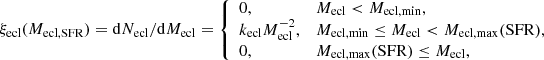 (1)
(1)
where Necl and Mecl are the number and the stellar mass of an embedded cluster and kecl is the normalisation factor accounting for the total mass of the embedded clusters that formed in the galaxy in a single star formation epoch of about 10 Myr. The lower mass limit of the ECMF, Mecl, min = 5 M⊙, is about the mass of the smallest stellar groups observed (Kroupa & Bouvier 2003; Kirk & Myers 2012). The upper mass limit of the ECMF is calculated as a function of the instantaneous SFR:
 (2)
(2)
where A = 4.83 and B = 0.75. This formulation has been determined by Weidner et al. (2004) to be consistent with the observed extragalactic Mecl, max − SFR relation (see also Randriamanakoto et al. 2013), where the parameter values are provided with uncertainties. We note in addition that the newest IGIMF formulation developed in Schulz et al. (2015) and Yan et al. (2017, their Eqs. (11), (12), and Fig. 2) has moved to a more generalised formulation without the need of introducing parameters A and B. However, because Eq. (2) was used by Lacchin et al. (2020), we implemented it as well for the purpose of an unbiased comparison of our results.
We note that SFR ⪅ 3.2 × 10⁻⁶ M⊙ yr−1 leads to a numerical inconsistency because Mecl, max would be smaller than Mecl, min = 5 M⊙ according to Eq. (2). This means that we cannot reproduce the SFHs of Lacchin et al. (2020), who obtained lower SFR values.
Here we decided to set the SFR to zero when the calculated SFR < 3.5 × 10⁻⁶ M⊙ yr−1. The typical timescale for a star cluster to form is approximately 1 Myr. When the SFR is this low, the number of stars that formed in about 1 Myr is so small that the IMF can no longer be treated as a smooth and continuous function. We refer to the discussion of extremely low SFRs with SFR ⪅ 10−6 M⊙ yr−1, the associated phenomenon of Hα dark star formation, and the associated maximum stellar masses that can form in Pflamm-Altenburg et al. (2007). At extremely low SFRs, the formation of individual stars affects the observational tracers. The IGIMF theory can account for this because instead of using the smooth gwIMF in integrated form, the formation of individual stars can also be traced (Yan et al. 2017, OSGIMF module of the GalIMF code).
These different treatments for low-SFR time steps in our calculation and that of Lacchin et al. (2020) are not expected to have a significant effect on the result because they are only related to a small fraction of stars. To be specific, the suggested SFT of Boötes I is shorter than 1 Gyr. Thus, the largest error on the modelled mass made by neglecting low SFR activities is ΔM = SFR ⋅ SFT < 3.5 × 10⁻⁶ M⊙ yr−1 × 10⁹ yr < 3.5 × 10³ M⊙, which is similar to the observational uncertainty in the mass of Boötes I (see Table 1). The metal yield of these low SFR populations is more negligible because they are exclusively composed of stars with a lower mass (⪅3 M⊙ according to the OSGIMF module of the GalIMF code) and have a longer lifetime (⪆400 Myr).
Input parameters and computation results of our best-fit chemical evolution models assuming the different IGIMF formulations introduced in Sect. 3.1 (lines 3 to 6) compared with the observational values (first line) and Lacchin et al. (2020) (second line).
The IMF of stars in an embedded cluster, ξ⋆, is assumed to be a two-part power-law function with its slope a function of metallicity and its upper mass limit a function of Mecl,
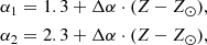
![Mathematical equation: $$ \begin{aligned}&\xi _{\star }(m,M_{\rm ecl,[Fe/H]}) = \mathrm{d} N_{\star }/\mathrm{d} m\nonumber \\&\qquad ={\left\{ \begin{array}{ll} 0,&m<0.08\,M_{\odot }, \\ k_{\rm \star } (m/0.5\,M_{\odot })^{-1.3},&0.08\,M_{\odot } \le m<0.5\,M_{\odot }, \\ k_{\rm \star } (m/0.5\,M_{\odot })^{-\alpha (\mathrm{[Fe/H]} )},&0.5\,M_{\odot } \le m < m_{\mathrm{max} }(M_{\rm ecl}), \\ 0,&m_{\mathrm{max} }(M_{\rm ecl}) \le m, \end{array}\right.} \end{aligned} $$](/articles/aa/full_html/2020/05/aa37567-20/aa37567-20-eq4.gif) (3)
(3)
where N⋆ and m are the stellar number and mass. The k⋆ is a normalisation factor. The power-law index α is calculated as
![Mathematical equation: $$ \begin{aligned} \alpha = 2.3 + 0.0572 \cdot \mathrm{[Fe/H]} . \end{aligned} $$](/articles/aa/full_html/2020/05/aa37567-20/aa37567-20-eq5.gif) (4)
(4)
We note that Eq. (4) (used by Recchi et al. 2014; Lacchin et al. 2020) differs from the original Marks et al. (2012) formulation, which additionally depends on density and holds only for stars more massive than 1 M⊙. The calculation of the upper stellar mass limit, mmax, in Eq. (3) is not mentioned clearly in Lacchin et al. (2020) but we assume that they followed Eqs. (3) and (4) of Recchi et al. (2009), and so do we.
Finally, the gwIMF, ξIGIMF, is the integration of the IMF of all the embedded clusters that form in the time interval δt = 10 Myr (see Axiom 5 in Yan et al. 2017, their Sect. 2.1),
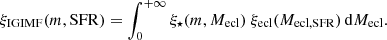 (5)
(5)
3.2. IGIMF theory as a framework
The IGIMF theory is not a specific IMF formulation, but a framework (the mathematical procedure described by Eq. (5)) that allows the computation of the gwIMF based on the empirically constrained ξ⋆ (the constraints are given in e.g. Kroupa 2005; Marks et al. 2012; Wang 2020) and ξecl (Lada & Lada 2003). Because the variation of the IMF in individual embedded clusters is still uncertain, as is the mass distribution function of the embedded star clusters, the IGIMF theory (Eq. (5)) can lead to different gwIMFs depending on the assumptions made for ξ⋆ and ξecl.
This does not mean that the IMF (ECMF) formulation can be adjusted to fit just any observation. On the contrary, the independent IMF constraints for low- and high-mass stars (e.g. the observational studies of the IMF in the Milky Way, and spectral features that are sensitive to the dwarf-to-giant ratio, as well as the UV-Hα luminosity ratio of other galaxies) need to be fulfilled. In addition, the resulting gwIMF calculated by the IGIMF theory has to be consistent with the observed galactic mean metallicity in the chemical evolution model where the SFH is determined by other observational constraints. For example, if the gwIMF assumption is more top-light, it has to be also more bottom-light in order to maintain the same resulting mean stellar metallicity, as is discussed in Sects. 6.5 and 6.6 below.
Three different IGIMF formulations (different assumptions on ξ⋆ and ξecl) are summarised in Jeřábková et al. (2018): their IGIMF1 formulation does not assume any IMF variation such that the gwIMF variation is purely due to the IGIMF theory; their IGIMF2 formulation considers that the IMF of massive stars depends on the cloud core density and metallicity; and their IGIMF3 model considers in addition that the IMF of low-mass stars depends on the gas metallicity (as supported by empirical evidence such as provided by Martín-Navarro et al. 2015). Different from Eq. (3), the assumed power law ξ⋆ in Jeřábková et al. (2018) changes not only at 0.5 M⊙, but also at 1 M⊙, and therefore has the form
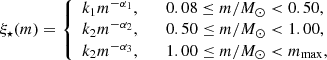 (6)
(6)
with
![Mathematical equation: $$ \begin{aligned} \alpha _1&=1.3+0.5\cdot [Z],\nonumber \\ \alpha _2&=2.3+0.5\cdot [Z],\nonumber \\ \alpha _3&=\alpha _3(\mathrm{[Z]} , M_{\rm ecl}), \end{aligned} $$](/articles/aa/full_html/2020/05/aa37567-20/aa37567-20-eq8.gif) (7)
(7)
where [Z] = log10(Z/Z⊙) and Z is the metal mass fraction of the star-forming molecular cloud. That is, α1 and α2 are functions of the metallicity, while α3 is a function of both metallicity and the initial stellar mass of a star cluster (see Jeřábková et al. 2018 their Eqs. (6) and (9) for the exact formulation of α3). In addition, Jeřábková et al. (2018) assumed for all their models a ξecl with a variable slope depending on the galaxy-wide SFR (see Weidner et al. 2013; Yan et al. 2017; Jeřábková et al. 2018, their Eq. (2)).
The IGIMF-R14 formulation leads to a gwIMF that is in between the IGIMF1 and IGIMF2 formulations because the IMF and ECMF variation exists in IGIMF-R14, but is much weaker than in the IGIMF2 formulation. This work mainly demonstrates the results of the default IGIMF-R14 model, but the more recent IGIMF formulations published in Yan et al. (2017) and Jeřábková et al. (2018) are also tested in Sect. 6.6.
We here used the notation IGIMF(Ai, i = 1, 2, …), where IGIMF(A1) = IGIMF1, IGIMF(A2) = IGIMF2, and IGIMF(A3) = IGIMF3 in the previous notation introduced in Jeřábková et al. (2018). This new notation represents the fact that the IGIMF theory, that is, the gwIMF, is an integration of all the embedded star cluster IMFs (Kroupa & Weidner 2003), which remains unchanged but acts on different assumptions, Ai (i = 1, 2, 3), on how the embedded cluster IMF varies, that is, on the mathematical definition of how the IMF in embedded star clusters depends on the metallicity and density of the star-forming molecular cloud core.
Every one of these Ai formulations is consistent with the star formation observed in the Milky Way. They only differ in the mathematical description under extreme star formation environments, which are not well constrained to date. For example, IGIMF(A3) allows for the IMF to vary with metallicity for massive stars as well as for low-mass stars that are empirically constrained by indirect evidence such as dynamical simulations and spectral features.
Furthermore, in Sect. 6.6 below, we use the observation of UFD Boötes I to provide new constraints on the variation of the IMF for low-mass stars at low metallicity. These new constraints are presented as assumption A4 (Eq. (8)). We emphasise that we do not adjust the general IGIMF theory to force improved agreement with the data, but that we use the galaxy-wide data of the UFD Boötes I, which represents an extreme star formation environment, to improve our knowledge on parsec-scale star formation in this environment. Whether this A4 formulation is correct can be tested using other UFDs, subject to the constraint that the formation history of these may differ, however.
3.3. Galaxy chemical evolution model
The chemical evolution of a dwarf galaxy is calculated using the galaxy chemical evolution model described in Yan et al. (2019), applying most of the same assumptions as Lacchin et al. (2020). Here we describe the model modifications and initial settings for this particular study and refer to Yan et al. (2019) for a detailed and comprehensive description of the galaxy chemical evolution model.
The SFR at a given time step is determined by the instantaneous gas mass of the galaxy following a linear relation (Lacchin et al. 2020, their Eq. (10)). That is, the gas mass of a galaxy divided by its SFR is assumed to be a constant τg (the gas-depletion timescale defined in Pflamm-Altenburg & Kroupa 2009), which is also the reciprocal of the star formation efficiency parameter, ν, discussed in Lacchin et al. (2020). This basically leads to a constant SFR over time before the onset of the galactic wind or any other mechanism that removes the galactic gas efficiently because the gas mass transformed into stars is much smaller than the total gas mass.
A simplification of our model is that all gas exists in the galaxy at the initial time, with a total gas mass being Mini, while Lacchin et al. (2020) applied a short gas infall timescale. These treatments are equivalent to each other in this particular case because their suggested gas-infall timescale for Boötes I is only 5 Myr, which is shorter than the smallest time step of our model, δt = 10 Myr.
We adopted the stellar yield of massive stars from Kobayashi et al. (2006). However, we only adopted the yield table for metallicity Z = 0.02, 0.004, and 0. For stars with an initial metallicity above 0.02, we applied the Z = 0.02 yield table, while for stars with an initial metallicity below 0.02, we used an interpolated value. We note that this is different from Yan et al. (2019), where the yields were only interpolated as a function of stellar mass instead of being interpolated as a function of both stellar mass and initial metallicity.
For the low- and intermediate-mass stars, our applied yield table from Marigo (2001) is different from the one adopted by Lacchin et al. (2020). Because the SFT of our best-fit model is short, which means low-mass stars do not participate in the chemical evolution of the galaxy.
We adopted the SNIa yield table from Iwamoto et al. (1999, their W70 model). The contribution to metal enrichment by SNIa was included in galactic chemical evolution models for the first time by Matteucci & Greggio (1986) with a numerical formulation. The explosion of SNIa follows certain delay-time distribution functions (DTD). An analytical DTD was first introduced in Greggio (2005). Here we tested two different DTDs, one is an empirical function, and the other is a physically motivated function.
The empirical power-law DTD suggested by Maoz & Mannucci (2012, see their Eq. (13) and Fig. 7) was applied as our default model. With this DTD, the SNIa rate peaks at 40 Myr after a single stellar population forms such that the DTD for all stellar population peaks at about SFT plus 40 Myr. The resulting DTD peak in our model is earlier than that of Lacchin et al. (2020) as is shown in Fig. 3. This difference does not affect our conclusions (see below). The computation results assuming the power-law DTD are shown in Sect. 5.
In addition, the solution with the physically motivated DTD applied by Lacchin et al. (2020) is discussed in Sect. 6.2. Considering that the shape of the real DTD is likely to have a little plateau at early times according to the single-degenerate or double-degenerate SNIa model (see e.g. Matteucci et al. 2009), it is necessary to test the single-degenerate DTD formulation given by Matteucci & Recchi (2001, their Eq. (2)) and applied by Lacchin et al. (2020). The computation results assuming the single-degenerate model are shown in Appendix A.
In both of these DTD models, the total number of SNIa events from a given stellar population depends not only on the mass of the stellar population, but also on its IMF. The gwIMF is no longer a power law when the IGIMF theory is applied, and the number of potential SNIa precursors is different from that in a canonical IMF. It is important to calculate the SNIa number and needs to be documented clearly in the models that apply a non-canonical IMF. For the power-law DTD, a correction to the number of SNIa events is made according to the number of stars with a mass between 1.5 and 8 M⊙ as explained in Yan et al. (2019, their Eq. (4)). For the single-degenerate DTD, we applied that of Matteucci & Recchi (2001, their Eq. (2)), where the mass function therein, ϕ, is the gwIMF calculated by the IGIMF theory.
Because the existence of dark matter particles remains speculative (Kroupa 2012, 2015), we refer to the phantom dark matter, which is the Milgromian gravitational force (Famaey & McGaugh 2012; Lüghausen et al. 2013, 2015), but parametrised here, for the sake of comparison with Lacchin et al. (2020), in the same way as dark matter. A (phantom) dark matter halo mass of 3 × 10⁶ M⊙ (Collins et al. 2014), an effective radius of the luminous (baryonic) component of 242 pc (Martin et al. 2008), and a ratio between the half-light radius and the (phantom) dark matter halo effective radius of 0.3 (Lacchin et al. 2020) was assumed.
With a given initial baryonic mass, a nominal gas-binding energy can be estimated using its current-day effective radius, current-day (phantom) dark matter halo, and applying the formulations given in Bradamante et al. (1998).
We note, however, that by assuming the estimated (phantom) dark matter mass as an invariant, the gas dominates the galaxy mass initially because the initial gas mass of our best-fit solution is about 4 × 10⁶ M⊙ and the best-fit infall gas mass of Lacchin et al. (2020) is above 107 M⊙. It is possible that the galaxy loses most of its gas and also its dark matter halo through tidal stripping such that the applied gas-binding energy is underestimated. This tidal-stripping scenario is no longer consistent with the galactic wind assumption (see paragraphs in below and Sect. 7.2) and is beyond the scope of a chemical evolution model, which only constrains the baryonic matter and SFH.
The nominal binding energy was then compared with the total energy deposited in the gas by type II supernova (SNII) and SNIa events to determine whether a galactic wind develops. Because the gas-binding energy changes insignificantly through the mass transfer between gas and stars compared to the energy generated by the stars, we considered the nominal binding energy a constant for the current purpose and calculated only the initial gas-binding energy.
Every star above 8 M⊙ is assumed to explode as a SNII at the end of its life. Each SNII and SNIa is assumed to pass a kinetic energy of ηSNII × 1051 erg and ηSNIa × 1051 erg to the gas phase, respectively. Following Bradamante et al. (1998) and Yin et al. (2011), the thermalisation efficiency of SNII and SNIa is ηSNII = 0.03 and ηSNIa = 0.8, respectively. The parameter ηSNII probalby lies in between 0.01 and 0.1 (Romano et al. 2015), while the parameter ηSNIa can be higher because SNIa occur at a later time in a hotter and more rarefied medium (Yin et al. 2011). These uncertainties affect the predicted onset time of the galactic wind. Stellar winds also deposit energy to the gas but is about two orders of magnitudes lower than the energy deposited by the supernova (Bradamante et al. 1998; Romano et al. 2015) and can therefore be safely neglected.
The galactic wind model was implemented according to Lacchin et al. (2020, their Eq. (12)). In this model the galactic mass loss is given by the SFR multiplied by the wind efficiency factor ω. The galactic wind is launched when the accumulated energy deposited by the supernovae exceeds the nominal galactic binding energy. When this occurs, the uniformly mixed gas begins to be removed at a rate of ω ⋅ SFR from the model at each time step.
We note that the assumed behaviour of the galactic wind is a very simplified model. As discussed in Sects. 7.2 and 7.5, the gas removal from UFDs is probably due to environmental effects in addition to stellar feedbacks (Romano et al. 2015, 2019). Thus, ω is a mathematical simplification used to formulate any possible physical mechanism that leads to the gas removal of UFD Boötes I and the consequent quenching of the star formation. In addition, ω is not a free parameter in our model. The only purpose of ω or the only criteria we applied to determine its value is that our code reproduces the SFH presented in Lacchin et al. (2020, their Fig. 3), when the same assumptions are applied. The choice of ω is ultimately justified by comparing the resulting best-fit SFH with the SFH estimated from the CMD data which indicates a single starburst and short SFT (Sect. 7.5).
4. Input parameters
Our models use two free parameters, τg and Mini, to fit the [α/Fe]–[Fe/H] relations and final galaxy mass, following these steps:
– τg: The gas-depletion timescale determines the SFT, that is, how spread out in time the SFH is for a fixed total stellar mass. Based on the shape of the top part of the IMF and the SFT, the shape of the [α/Fe]–[Fe/H] evolution tracks (i.e. the [Fe/H] value when SNIa start to have a significant influence on [α/Fe]) is determined as described in Lacchin et al. (2020). For a given observed [α/Fe]–[Fe/H] relation, a more top-light gwIMF requires a shorter τg to fit the relation.
A short τg (or large ν = 1/τg) is not unprecedented for dwarf galaxy studies (cf. Lanfranchi et al. 2006; Vincenzo et al. 2015). The conclusion that UFDs have a much longer τg than dwarfs stems from the chemical evolution models assuming the Salpeter gwIMF (Vincenzo et al. 2014; Romano et al. 2015), but this conclusion depends on the IMF.
The parameter τg can only fit the average [α/Fe]–[Fe/H] relation for the α elements, while the individual [α/Fe]–[Fe/H] relations for different α elements depend on the literature stellar yield tables, the SNIa yield, and the DTD of SNIa events.
– Mini: The galaxy initial mass (with a baryon gas mass of Mini and a constant phantom dark matter mass) and radius determine the galactic potential, and thus how many stars are formed until the total energy production from supernovae is equal to the gas binding energy, which determines the onset time of the galactic wind. With the resulting number of SN for a computed gwIMF, the total stellar mass formed and the final living stellar mass, M*, final, of the galaxy is determined. In other words, a higher Mini leads to a deeper galactic potential that allows the formation of more stars before the star formation activity is quenched by the energy feedback. Such behaviour of the model depends on the assumption that the star formation is quenched by the galactic wind.
Our best-fit model has a lower Mini and a shorter τg than the parameters applied in Lacchin et al. (2020) of all their models (their 1BooI to 6BooI). The input parameters are listed in Table 1.
We note that the model suffers from the limited time resolution of the galaxy chemical evolution model when our best-fit SFT is a few 10 Myr, while the shortest time step in our model is δt = 10 Myr. That is, all stars that formed within the first 10 Myr time step, not an negligible fraction of the entire stellar population, have zero metallicity in our model even if some of them might already be enriched in reality.
Because the gwIMF depends on the gas metallicity using the IGIMF-R14 formulation, we must artificially define the logarithm of the metallicity of the first time step to be [Z] = − 7 instead of [Z] = − ∞. This time step effectively introduces some uncertainty to our results. However, we considered the choice of initial metallicity to not be a free parameter of our model because (1) the galaxy metallicity of the second time step is about [Z] = − 4 regardless of the initial metallicity, such that the initial metallicity must be lower than [Z] = − 4; and (2) the IGIMF formulation is supported by empirical evidence for [Z]⪆ − 4. The resulting gwIMF can no longer be trusted when [Z] is much lower (as discussed in Sect. 6.6 below). Therefore, to mimic zero initial metallicity, we considered [Z] = − 7 a reasonable choice.
We emphasise the importance of exploring a parameter space that is large enough. While full blind numerical exploration would be very challenging computationally, we present a systematical way of exploring physically plausible values of input parameters. Our recovered input parameters, with which the model fits the observations, are outside of the explored parameter space of Lacchin et al. (2020).
Because the computational cost is so high, we did not optimise the model numerically. Our model agrees well with the data (see next section), and thus fulfils the aim of this work: to investigate whether it is possible to reproduce the observed properties of Boötes I naturally within the IGIMF framework.
5. Results
The solution of our default model, IGIMF-R14, was calculated following the procedure explained in Sect. 4. The resulting SFH, SNII, and SNIa rates, the accumulated gwIMF of each time step, and galaxy mass and energy evolution are shown in Figs. 1–6, where they are compared with the 3BooI-IGIMF model of Lacchin et al. (2020) if a similar plot is provided in their paper. The resulting [α/Fe]–[Fe/H] evolution tracks and final galaxy mass fit the observations well, as is shown in Fig. 7 and Table 1, respectively. The final galaxy mass lies within a 0.83σ uncertainty range of the observed value.
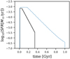 |
Fig. 1. SFHs. The SFH of the best-fit IGIMF-R14 model adopting the parameter set in Table 1 is shown with the black line. The SFH is shown as a histogram because the smallest time step is 10 Myr. The starting time of the galactic wind is 50 Myr (cf. Fig. 5), while the SFR drops to half of its peak value at about 90 Myr, which defines the SFT. The blue dashed line is the blue dashed line in Lacchin et al. (2020, their Fig. 3), i.e., their 3BooI-IGIMF model. |
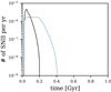 |
Fig. 2. Evolution history of the SNII rate. Similar to Fig. 1, but for the SNII rate of the best-fit IGIMF-R14 model. The initial spike SNII rate is due to the discontinuous 10 Myr time step where the metallicity increases from [Z] = − 7 to [Z] = − 4 at the second time step that leads to a sudden change in gwIMF according to the IGIMF-R14 formulation (see Fig. 4). The blue dashed line is the blue dashed line in Lacchin et al. (2020, their Fig. 5), i.e., their 3BooI-IGIMF model. |
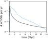 |
Fig. 3. Evolution history of the SNIa rate. Similar to Fig. 1, but for the SNIa rate of the best-fit IGIMF-R14 model. The blue dashed line is the blue dashed line in Lacchin et al. (2020, their Fig. 4), i.e., their 3BooI-IGIMF model. We note that the horizontal axis is different from Fig. 2. We also tested the DTD assumption of Lacchin et al. (2020) in our IGIMF-R14-SD model, shown in Fig. A.3. |
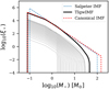 |
Fig. 4. Cumulative (time-integrated) gwIMF (TIgwIMF) for all stars ever formed (thick solid line) and the gwIMF for each 10 Myr star formation epoch (thin solid lines, evolving from the top to the bottom as time progresses) of the best-fit IGIMF-R14 model, compared with the canonical IMF and the Salpeter IMF. We note that the gwIMF for the first epoch (the highest thin gwIMF line) has a significantly higher maximum stellar mass limit than the second epoch. This is only because the initial metallicity was assumed to be Z = 0.02 × 10⁻⁷ and because the 10 Myr time step is unresolved. |
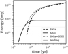 |
Fig. 5. Evolution of energy deposited in the gas by supernovae of the best-fit IGIMF-R14 model, compared to the (initial) nominal gas-binding energy assuming that the galactic radius and (phantom) dark matter mass does not evolve significantly (see Sect. 3.3). The galactic wind develops at the time step after the energy in gas exceeds the nominal binding energy. |
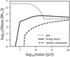 |
Fig. 6. Mass evolution of gas, living stars, and stellar remnants of the best-fit IGIMF-R14 model. The gas mass stops to decrease at about 108.5 yr, when the star formation and the corresponding galaxy wind stops, and remains constant thereafter. The amount of remaining gas mass is discussed in Sect. 5. |
The final gas mass shown in Fig. 6 represents an upper limit because the gas-mass value is subject to the assumed gas-removal mechanisms that are not taken into account in our computation. In reality, mechanisms such as tidal stripping would additionally remove the gas.
To determine whether the best-fit τg is consistent with the observation of dwarf galaxies, it is important to recall that the observational gas-depletion timescale depends on the gwIMF assumption because galaxy mass and galaxy SFR estimate both depend on the assumed gwIMF. Therefore we must consider the gas-depletion timescale estimate by applying the IGIMF theory. This is given in Pflamm-Altenburg & Kroupa (2009). The estimated gas-depletion timescale for star-forming dwarf galaxies becomes shorter when the IGIMF theory is assumed because their gwIMF is expected to be top-light, which means that more stars are forming per observed Hα or UV photon than in the estimation assuming the canonical or Salpeter IMF (see Fig. 4 for a comparison of different IMFs).
The best-fit τg is almost at the centre of the gas-depletion timescale distribution of a set of local star-forming galaxies given in Pflamm-Altenburg & Kroupa (2009, their Fig. 8), who calculated the observational τg assuming the IGIMF theory. This shows that our estimate from chemical abundances is consistent with the estimate from measuring the galactic SFR and gas mass of star-forming galaxies. This self-consistency when the IGIMF theory is applied is encouraging.
The corresponding SFT of the best-fit model also agrees with the morphology of the CMD and the required minimum SFT indicated by the metal distribution of the stars. Brown et al. (2014) showed that the two-stellar-component best-fit stellar populations have an age difference of 0.1 Gyr, with one population contributing 97% of the stellar mass. This indicates that Boötes I is likely to have formed in a single starburst on a timescale shorter than 100 Myr, in agreement with Okamoto et al. (2012) and Webster et al. (2015).
Finally, we determined whether our galactic stellar mean [Fe/H], [Fe/H]mean, agrees with the observation. The result from the best-fit IGIMF-R14 model is listed in Table 1. It is within a 1.75σ uncertainty range of the observed value.
Compared to the fitting results assuming the Salpeter gwIMF provided by Lacchin et al. (2020), our model assuming IGIMF-R14 fits the observations better. The goodness-of-fit for the [α/Fe]–[Fe/H] relations is similar in our model and the Salpeter model of Lacchin et al. (2020), as shown in Fig. 7. However, our M*, final and [Fe/H]mean fit the observational constraints better than the results given in Lacchin et al. (2020, their Table 3).
 |
Fig. 7. Evolution of [α/Fe]–[Fe/H] relations of the best-fit IGIMF-R14 model (black solid line). The circles are the data of Boötes I collected in Lacchin et al. (2020, their Fig. 6). The dashed line and the dash-dotted line are the two 3BooI models in Lacchin et al. (2020, their Fig. 6), assuming the gwIMF given by IGIMF-R14 and the Salpeter IMF, respectively. |
This shows that the IGIMF theory leads to a remarkably simple and self-consistent understanding of the Boötes I UFD galaxy.
6. Discussion
6.1. Number of SNIa events
The total numbers of SNIa events per unit total stellar mass for the modelled Boötes I UFD galaxy, NSNIa, gal, are listed in Table 1. These values can be compared, although they are not be constrained, by the estimated value from the local universe (Maoz & Mannucci 2012). NSNIa, gal at a given time was calculated by adding up the SNIa events from each star formation epoch of duration δt = 10 Myr. The number of SNIa events for each epoch depends on the mass of formed stars and the gwIMF of that epoch.
Maoz & Mannucci (2012), assuming an invariant IMF (defined as the “diet-Salpeter IMF”), applied a normalisation parameter for the DTD of a single star formation epoch, NSNIa, of 2 and 2.2, which is the number of SNIa per 1000 M⊙ of stars formed in 10 Gyr, in their Eq. (13) and Sect. 4.2, respectively, while Yan et al. (2019) applied NSNIa = 2.25. Here we follow Maoz & Mannucci (2012, their Sect. 4.2), for the default power-law DTD model, that is, NSNIa = 2.
We note that the GalIMF code applies a numerical integration of the IMF to calculate NSNIa, which differs from the analytical result with an error of about ±3%. Numerical integration is necessary when the gwIMF is no longer a power-law function according to the IGIMF theory. In addition, the observational uncertainty of NSNIa is large (e.g. 2 ± 0.6 in Maoz & Mannucci 2012, their Table 1). A change in the normalised number of SNIa leads to a significant difference in the resulting mean stellar [Fe/H]. As we have tested, a difference of one or two sigma between the model and observational mean stellar [Fe/H], which is only about 0.1 dex, can be caused by a NSNIa difference of a few percent (i.e. 2 ± 0.1).
Although the SNIa events affect the MDF differently than SNII events such that the [Fe/H] distribution of the observed stars can in principle constrain NSNIa, the MDF needs to be subjected to the same observational biases when it is compared to the stellar observed one. For example, the galactic abundances are largely based on the measurements of bright giant stars, but these constitute a relatively narrow stellar age window, while the real MDF may have a different mean value, be more spread out, and have a different shape.
Because the observational bias that may affect the shape of the MDF has not been studied in detail, it is not reliable to constrain the NSNIa with the shape of MDF.
6.2. DTD of SNIa events
The DTD of SNIa events is uncertain and still under debate. There are two main groups of DTD formulations described by power-law functions and exponential functions, where the power-law DTDs are more peaked at early times (see DTD comparisons e.g. in Strolger et al. 2020; Matteucci et al. 2009). Here we tested two commonly applied DTD formulations belonging to these two groups, one of which is the formulation applied by Lacchin et al. (2020), to explore the potential influence of the DTD assumption on our conclusions.
Our default model, IGIMF-R14, closely follows the assumptions of Lacchin et al. (2020), but assumes the power-law DTD described in Sect. 3.3 and shown in Fig. 3. The SNIa rate peaks at about 130 Myr in the IGIMF-R14 model here (which is roughly SFT + 40 Myr), while it peaks at about 350 Myr for the model shown in Lacchin et al. (2020), that is, the blue dashed line in Fig. 3.
The apparent difference in the SNIa event distribution shown in Fig. 3 is not only due to the difference in DTD of the single stellar population, but also due to the difference in the SFH (Fig. 1).
The different DTD affects the best-fit SFT because it is the SFT relative to the peak SNIa rate timescale that determines the shape of the [α/Fe]–[Fe/H] relations. This means that applying a different DTD would not change the fact that a solution is possible, but the corresponding metal-enrichment history would be different.
To ensure a fair comparison and demonstrate the effect of assuming an alternative DTD, we tested the DTD applied by Lacchin et al. (2020) in our model IGIMF-R14-SD.
IGIMF-R14-SD applied the single-degenerate DTD formulation of Matteucci & Recchi (2001, their Eqs. (2)–(5)), with the parameters therein, MBm = 3 and γ = 2. The total number of SNIa was normalised (with the parameter A in Matteucci & Recchi 2001) such that the GalIMF code reproduces the 3BooI-Salpeter model of Lacchin et al. (2020), which resulted in the same SFH and SNIa rate evolution history.
According to the single-degenerate SNIa model assumption (Greggio & Renzini 1983), the SNIa rate is determined by the death rate of the companion star with a mass M2 (while the initial mass of the primary star is M1). To obtain all SNIa events, we therefore need the mass distribution of the companion stars,  , and the lifetime function. The mass distribution of the companion stars is calculated by integration over the possible total masses of binary systems (MB = M1 + M2) that possess a secondary star with mass M2 modulated by a probability function of having such a binary system given the value M2/MB.
As discussed for example in Kroupa & Jerabkova (2018), the IMF of the binary systems (their “the IMF of unresolved binaries”) is similar to the IMF of single stars. When the SNIa rate is calculated, it is therefore reasonable to use the gwIMF calculated for the single stars at a given time as the IMF of the MB.
The calculation results of model IGIMF-R14-SD are shown in Table 1 and Appendix A.
The results of model IGIMF-R14 and IGIMF-R14-SD applying two different DTDs both fit the observational values well and within about two standard deviations (Figs. 7 and A.7, and Table 1).
Notably, the observational value is in between the results of these two models, indicating that the IGIMF-R14 formulation agrees with the data with a reasonable DTD assumption.
6.3. Galaxy age
The galaxy evolution model stops at a certain time, according to the estimated age of Boötes I, and generates model outputs. The stopping time needs to be specified before the simulation begins. Here we set the modelled galaxy to be 14 Gyr old.
Through a CMD fitting analysis, Boötes I is found to be dominated by an old single stellar population of age = 14 ± 2 Gyr according to de Jong et al. (2008), of about 13.7 Gyr according to Okamoto et al. (2012), and of 13.3 ± 0.3 Gyr according to Brown et al. (2014).
The uncertainty of the age estimation comes from the uncertainty of the isochrone model and the metallicity assumption of the applied isochrone (Coelho et al. 2020). The metallicity and α-enhancement of the real stellar population are not exactly the same as the assumed isochrone.
As the galaxy becomes older, its living stellar mass (Fig. 6) and mean stellar [Fe/H], which we compared with the observed values, slowly decreases. An age difference of about 1 or 2 Gyr does not have a significant effect on the results of the galaxy evolution model.
6.4. Final mass of living stars
The mass of living stars at 14 Gyr in our model is compared and fitted with the observational stellar mass of Boötes I by modifying the input parameter Mini as described in Sect. 4.
The observational stellar mass of Boötes I estimated by Martin et al. (2008) depends on the assumed gwIMF, and in particular on the gwIMF of low-mass stars because the galaxy in question is about 13.7 Gyr old.
Here we compared our result with the stellar mass estimation assuming the canonical IMF because the IGIMF-R14 formulation, although its gwIMF changes systematically, also assumes a fixed canonical IMF for stars less massive than 1 M⊙. Thus the comparison is consistent.
The low-mass part of the IMF may also change depending on the metallicity of the star-forming region. Such a variation has been suggested by the observation of massive elliptical galaxies (e.g. van Dokkum & Conroy 2010; Martín-Navarro et al. 2015; Parikh et al. 2018) and already earlier by evidence gleaned from resolved stellar populations (Kroupa 2002; Marks et al. 2012; Jeřábková et al. 2018). The IGIMF theory in its most recent formulation (Jeřábková et al. 2018) predicts a bottom-light gwIMF for low-metallicity populations.
If the real gwIMF is indeed bottom-light, the estimated galaxy mass using the star number counts from Martin et al. (2008) would be lower, but the galaxy mass that best fits the [α/Fe]–[Fe/H] relation with our model will also be lower and therefore retain the consistency between our model and the observational mass.
6.5. Mean stellar [Fe/H]
We did not fit the stellar MDF (and its mean, [Fe/H]mean) here, it was predicted by the model. It can therefore be compared with the observations to test the model. We also refer to Sect. 6.1 for a discussion of the bias affecting an observed MDF, however.
Lacchin et al. (2020) compared their model prediction with the MDF, but we compared the model result only with the [Fe/H]mean as a representative measure of the full MDF.
Because only a few stars are observed (≈30) and available to construct the observational MDF, the mean is the most prominent and thus robust feature of the MDF. The second most prominent feature, the width of the predicted MDF, is not significantly changed relative to the observational width of the MDF under different input parameters (as was shown in Lacchin et al. 2020, their Figs. 8, 13, and 15). We argue that no useful information is lost when we compress the MDF into its mean. As a result, a mismatch of the MDF between model prediction and observation should be considered as a single mismatch of the mean stellar [Fe/H] instead of repeated failures for every single star.
We note that this simplification, although appropriate here, would not be appropriate in a study of galaxies with better constrained observational MDFs. In this case, the MDF provides useful information to constrain the galaxy chemical evolution model.
The resulting [Fe/H]mean of the IGIMF-R14 model agrees well with the observation (Lacchin et al. 2020) within the 1.75σ error range. The agreement may be undervalued because the observational estimate of [Fe/H] depends on the assumed [α/Fe] (e.g. Okamoto et al. 2012). Different groups give different [Fe/H] estimates, indicating a larger uncertainty of the observation. For example, de Jong et al. (2008, their Table 5), estimated that the best-fit [Fe/H] value for the CMD is −2.2 ± 0.2, which agrees perfectly with our default model IGIMF-R14. On the other hand, Lai et al. (2011) applied a low-resolution spectroscopic analysis and found that the mean [Fe/H] value of 25 stars is −2.59 (or −2.64 when the solar metallicity from Asplund et al. 2009 is assumed), which is much lower and may be more challenging to reproduce with our current model assumptions.
We note that the observational mean [Fe/H] from the above literature is a direct mean of [Fe/H] values inferred for the single stars, while [Fe/H]mean, the stellar iron abundance for the entire galaxy, is the mass-weighted [Fe/H] defined as [Fe/H]mean = log10(MFe/MH)−log10(MFe, ⊙/MH, ⊙), where MFe or MH are the total mass of iron or hydrogen in all the stars in Boötes I and MFe, ⊙ or MH, ⊙ are the total mass of iron or hydrogen in the Sun. This shows that the observational mean [Fe/H] and [Fe/H]mean are not exactly comparable. However, because only a few stars are observed, this difference is not usually mentioned (e.g. in Lacchin et al. 2020).
It is not trivial that the predicted [Fe/H]mean of our model agrees with the observation automatically because the procedure described in Sect. 4 only fits the [α/Fe]–[Fe/H] relation and the final living stellar mass. The following factors can all affect the final [Fe/H] significantly:
– gwIMF: For the same mass in final living stars, a stellar population with a bottom-light gwIMF produces more metals than the case for the canonical IMF and leads to a metal-rich galaxy.
– SFT: A shorter SFT leads to a lower metal mass returned to the gas before the end of the star formation era, which decreases the stellar metallicity.
– Galaxy mass: Given the initial galaxy mass, the gas-binding energy determines how many stars can form before the onset of the strong galactic wind, and thus how many metals can be produced by the stars. The mean metallicity of the galaxy is determined and depends on the galaxy mass because the binding energy is approximately proportional to the square of the galaxy mass, while the energy production from the supernovae is linearly related to the galaxy mass. This leads to a higher metallicity for a more massive galaxy.
Although the galaxy mass and SFT have been determined in the fitting procedure described in Sect. 4, the assumed gwIMF can still affect the final galactic metallicity. Thus the galaxy chemical evolution model can potentially falsify the applied IMF theory. The IGIMF-R14 formulation works well, however.
The fit can be improved further if the gwIMF is slightly more bottom-heavy (than the canonical IMF). This would be the case if the low-mass IMF slope were slightly steeper or if the minimum star cluster mass were slightly lower.
The IMF constraint for the low-mass stars has a large uncertainty; see for example Kroupa (2001, their Eq. (2)) and Sect. 6.6. Thus, our result is well consistent with the observation, signalling a fruitful potential of the IGIMF theory.
6.6. Other IGIMF formulations
Because the assumed IMF function affects the chemical evolution of the UFD Boötes I, we can use the observed properties of Boötes I to constrain the IMF formulation, that is, ξ* (Eqs. (3) and (4)). Instead of the default IGIMF-R14 formulation, here we test whether the IGIMF(A2) and IGIMF(A3) formulations (introduced in Sect. 3.2, Eqs. (6) and (7)) is consistent with the constraints given by Boötes I.
The [α/Fe]–[Fe/H] relation can be fitted regardless of the applied ξ* variation that is assumed. By adjusting τg, all the IGIMF formulations can develop a galactic wind at a similar time (Table 1) and thus fit the [α/Fe]–[Fe/H] relation. The required values of τg are also acceptable and agree well with the observational constraint (Table 1).
However, not every IGIMF formulation can fit the galaxy mass and metallicity simultaneously, as explained in Sect. 6.5 above. The best-fit IGIMF formulation appears to be in between the IGIMF(A2) and IGIMF(A3) formulations. When a modification of the low-mass IMF slope is allowed, that is, one more free parameter, all the considered observations can be fitted perfectly. This means that the low-mass IMF formulation is constrained by the high-mass IMF (IMF of the stars with a mass higher than 1 M⊙) and the observation of UFDs.
The best-fit IGIMF formulation, IGIMF(A4), assumes that the power-law index of the low-mass IMF, α1 and α2 in Eq. (6), varies with metallicity according to
![Mathematical equation: $$ \begin{aligned} \alpha _1=1.3+0.12\cdot [Z],\nonumber \\ \alpha _2=2.3+0.12\cdot [Z], \end{aligned} $$](/articles/aa/full_html/2020/05/aa37567-20/aa37567-20-eq10.gif) (8)
(8)
instead of Eq. (7). This variation of α1 and α2 is smaller than the assumption applied in Marks et al. (2012), leading to a mildly bottom-light gwIMF.
The different multipliers of [Z] (0.12 in Eq. (8) while 0.5 in Marks et al. 2012, their Eq. (12)) can agree with each other if the IMF slope depends on the metallicity, Z, instead of [Z]. The latter is not reasonable when Z ≈ 0 because the IMF shape varies significantly from [Z] = − 10 to [Z] = − 100 even if Z is similar to zero for both cases.
We propose here a new formulation for the variation of the IMF power-law index for low-mass stars, that is, α1 for stars with masses lower than 0.5 M⊙ and α2 for stars with mass between 0.5 and 1 M⊙:
 (9)
(9)
where Δα ≈ 35 fits the observational M*, final and [Fe/H]mean best.
With Δα = 35, Eqs. (9) and (8) give the same α1 and α2 values when [Z] ≈ − 5.8 (the case for UFDs) and is consistent with Marks et al. (2012, their Eq. (12)), when [Z]≈ − 1.3 (the case for the Galactic GCs, Kroupa 2002). That is, the proposed formulation (Eq. (9)) based on new requirements from the UFDs is similar to the previous formulation (Eq. (8)) for the metal-rich regime such that it naturally fulfils the IMF constraints given by the GCs.
With better data at hand, the chemical evolution model of UFDs is therefore capable of providing constraints on IMF variations on the sub-parsec (embedded cluster) scale. Our prediction (Eq. (9)) can be compared with the low-mass gwIMF in Local Group dwarf galaxies, which will be better constrained with the James Webb Space Telescope (El-Badry et al. 2017).
7. Comparison with Lacchin et al. (2020)
This paper benefits greatly from Lacchin et al. (2020) and a long and detailed discussion with Francesca Matteucci (priv. comm.). We applied an almost identical set of assumptions and observational constraints. Lacchin et al. (2020) used a code by Lanfranchi & Matteucci (2004) with their implementation of the IGIMF-R14, and we used the publicly available code GalIMF that we developed previously (Yan et al. 2019) following a very similar set of assumptions and input parameters as Lacchin et al. (2020). While the two codes are not identical, they are expected to yield comparable results. However, we appear to draw contradictory conclusions. Here we discuss the differences in the model, fitting routine, results, and interpretation.
7.1. DTDs
As mentioned in Sect. 6.2, we tested the DTD formulation of the single-degenerate SNIa model formulated in Matteucci & Recchi (2001, their Eqs. (2)–(5)), to demonstrate the effect of applying an alternative DTD.
A different DTD model indeed affects the galactic mean metallicity significantly, but in a way that the observational value lies in between the IGIMF-R14 and IGIMF-R14-SD results such that both DTD models are consistent with observations within the 2σ uncertainty range.
These tests demonstrate the limitation of the chemical evolution models, where the conclusion depends on the as yet unknown nature of the SNIa. In the case of testing the IGIMF-R14 formulation, it happens not to change our conclusion that the IGIMF-R14 model reproduces the Boötes I data well (and naturally), however.
7.2. Set the wind efficiency
The wind efficiency parameter, ω, defined in Sect. 3.3, affects the stellar mass that is formed after the onset of the galactic wind. A lower wind efficiency leads to a higher galaxy stellar mass and metallicity.
Lacchin et al. (2020) claims that their modelled wind rate is proportional to the SFR, but in reality, their modelled wind rate is proportional to the amount of gas to prevent the wind from stopping when the SFR decreases to zero following Yin et al. (2011). We therefore cannot directly adopt the ω value reported in Lacchin et al. (2020), but have to find the equivalent ω that can reproduce their demonstrated SFH. We tested different values of ω and found that ω ≈ 100 results in a similar SFH.
This means that ω is applied only for a fair comparison with Lacchin et al. (2020). The strong loss of gas and the fast quenching of the SFH is justified by the stellar age and abundance distribution of the UFDs, as was demonstrated in Vincenzo et al. (2014), for example, but the physical mechanism for losing the gas is not necessarily a galactic wind, even though we call ω the “galactic wind efficiency parameter”. The appropriate value of ω as well as whether the “galactic wind” should depend on the SFR or the remaining gas mass therefore remains unsettled and unconstrained.
It has been suggested by Romano et al. (2015, 2019) that stellar feedback is not effective in removing all the gas from Boötes I and that an external mechanism, such as tidal or ram-pressure stripping, is needed. With the assumed formulation that the galactic wind rate is proportional to the SFR, any mechanism that leads to the gas depletion of Boötes I is parametrised by a high ω value.
The proper value of ω is unknown and expected to depend on the gwIMF. It is therefore expected to be time dependent. The best-fit solution can be affected when ω takes a different value, when the gas is removed from the galaxy not by the galaxy wind, but by an alternative mechanism (Romano et al. 2015, 2019), or if the suppression of star formation is not due to the gas depletion (Forbes et al. 2016; Lebouteiller et al. 2017).
7.3. Fitting routine
As a first step, we ensured that when we applied the same underlying assumptions and input parameters, our results and the results of Lacchin et al. (2020) were mutually consistent. The low-metal part of the [α/Fe]–[Fe/H] relations and especially the Ca abundance are not identical and require further investigation, but these differences mainly demonstrate the limitations and uncertainties of chemical evolution models and would not affect our conclusions. This is because it is not a challenge for a model to fit the [α/Fe]–[Fe/H] relations because this can almost always be done by tuning the gas-depletion timescale. The main challenge, on the other hand, is to simultaneously reproduce the observed M*, final and [Fe/H]mean (or MDF, in the case of Lacchin et al. 2020, see Sects. 6.1 and 6.5) of the galaxy.
As we explained in Sect. 4, there are two free input parameters but three independent observables. We fit M*, final within 1σ deviation of the observation by tuning the input parameter Mini, while the [Fe/H]mean was left to test the model. The resulting [Fe/H]mean of our model in which we apply the IGIMF theory naturally agrees with the observational values to within about 2σ, which represents the observations better than the models shown in Lacchin et al. (2020).
The fitting routine explained in Sect. 4 allows us to identify the input parameters that result in a good agreement with the data. While Lacchin et al. (2020) studied a sparse grid of input parameter sets, they did not contain or cover the best-fitting input parameters we found. This seems to be the main reason for our different conclusions.
7.4. [α/Fe]–[Fe/H] relations
As shown in Fig 7, the intrinsic scatter of the [α/Fe]–[Fe/H] data is large as a result of the complex galactic gas and metal distribution, and stars may form outside the main progenitor halo (Jeon et al. 2017). Our mean galactic metal evolution track assumes that all the gas is always well mixed and thus cannot explain the metal abundance of individual single stars.
The best-fit model that applies the IGIMF theory is comparable with the solutions given by Lacchin et al. (2020), which are shown as the dashed and dash-dotted lines in Fig 7, especially for metal-rich stars. The highest [α/Fe] value at the metal-poor end of the plots from Lacchin et al. (2020) is lower than our results and fits the data not as well as our model, however.
The highest [α/Fe] value should be the IMF-weighted [α/Fe] value of all the massive stars with Z = 0 and a lifetime shorter than the first time step, δt = 10 Myr, that is, the IMF-weighted thin solid line within the red shaded region of Fig. 8. Because the IMF-weighted value should be higher than the lowest value in the red region, it is clear that the initial [Mg/Fe] should be higher than 0.5, which agrees with our result and disagrees with Lacchin et al. (2020).
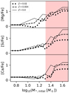 |
Fig. 8. Stellar metal yield ratios of stars with different mass and metallicity given by Kobayashi et al. (2006). The yields from Kobayashi et al. (2006) for massive stars are connected to the yields for low- and intermediate-mass stars as given by Marigo (2001). The yields for M* > 40 M⊙ are the same as the yields for M* = 40 M⊙ stars. The red shaded region with log10(M*, initial[M⊙]) > 1.3073 indicates zero-metallicity stars with lifetimes shorter than 10 Myr, according to Yan et al. (2019). |
The [α/Fe] plateau can be enhanced by a more complicated gas-flow model, a larger stellar-mass bin, or a larger model time step. A non-simultaneous star formation combined with local stellar wind pollution can also complicate the model prediction, which requires more elaborate hydrochemical simulations.
We note that the metal-poor part of the [α/Fe]–[Fe/H] relations is affected by the small number of stars that are formed at the earliest time steps. This shows that the metal-poor part is not reliable because of the small number of massive stars that affect it, the uncertainty of the stellar winds of these massive stars, and whether or not they explode as supernovae. Stars that are more massive than 40 M⊙ share the same adopted stellar yield table, which is certainly not the ideal setup to discuss the chemical abundance of the extremely metal-poor era of a galaxy.
7.5. Star formation history
The tested SFT in Lacchin et al. (2020) is generally longer than our best-fit models.
Because the gas flow and star formation criteria in the chemical evolution model are uncertain, the best-fit SFH is not conclusive. Here we compare it with the independently estimated SFH given by the CMD. Brown et al. (2014) demonstrated that the CMD of Boötes I is best fit by essentially a single starburst on a short timescale, in agreement with our result. We note that the cumulative SFH shown in Brown et al. (2014, their Fig. 8), is consistent with their best-fit model and our resulting SFH as well.
The short SFT required by our model to fit the [α/Fe]–[Fe/H] relations is thus supported by the SFH obtained from the CMD of Boötes I (Brown et al. 2014) and is consistent with the average gas-depletion timescale of dwarf galaxies (Pflamm-Altenburg & Kroupa 2009). Our results are also in line with Webster et al. (2015), showing that the shortest SFT required for the observed self-enrichment of the UFDs is about 0.1 Gyr. The gas of low-mass-satellite galaxies was removed by their interaction with the Milky May (Romano et al. 2015, 2019) such that they shut off star formation on a short timescale, as also found for Dragonfly 44 by Haghi et al. (2019).
In addition, we note that when the SFR drops low, the continued star formation activity does not have a great effect on the chemical abundances. When we assume that after the onset of the galactic wind and after each star formation epoch, the extremely diluted gas needs a cooling time of one to a few 10 Myr before forming new stars (Lebouteiller et al. 2017), then the SFH may be greatly extended, such as the one shown in Fig. 9. The resulting [α/Fe]–[Fe/H] relation, M*, final, and [Fe/H]mean are barely affected, however.
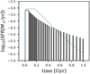 |
Fig. 9. SFH requiring an artificial gas-cooling time. The blue dashed line is the same as in Fig. 1. Compared to the best-fit IGIMF-R14 model (with the SFH shown in Fig. 1), the discretised SFH has a larger spread but similar galaxy evolution results (see Sect. 7.5). |
7.6. Interpretation of the result
Because there is still a 2σ mismatch between the model prediction and the observation, the question remains whether the 2σ difference excludes the assumed IGIMF-R14 formulation. We consider this an acceptable agreement because the uncertainty of the assumptions applied in the model (see below) can certainly cause a 2σ disagreement, that is, the discrepancy may not be due to an incorrect gwIMF assumption, but to errors in other assumptions.
For example, a lower dark matter mass and/or a higher ηSNII (0.1 instead of the 0.03 applied here, see Sect. 3.3, is possible, Bradamante et al. 1998; Romano et al. 2015) combined with a higher Mini would help reduce the value of [Fe/H]mean. Metal-rich gas ejected by the supernovae may be preferentially expelled from such a low-mass galaxy especially for off-centre explosions (Webster et al. 2014; Romano et al. 2015, 2019). Similarly, the galaxy radius at the onset time of the galactic wind may be different from its present-day radius. The DTD of SNIa explosions is uncertain and may peak at a different time (see Sect. 7.1). The stellar yield may be different and the massive stars may collapse to black holes without ejecting metals to the gas. Other assumptions in the model, such as the single-zone assumption or instantaneous-gas-mixing assumption, all affect the fitting results, and it is difficult to quantify how large the effect is.
7.7. Summary
In summary, we first reproduced the results of Lacchin et al. (2020, their model 3BooI), with the same assumptions and input parameters applied to ensure that the results from the two codes are in line and comparable. Then we determined a set of input parameters that led to a better model fit with the observations than the models in Lacchin et al. (2020). Finally, we discussed the various observational and model uncertainties and conclude that with the current accuracy, the IGIMF model describes the observed properties of Boötes I self-consistently and naturally, and in particularly better than the solution that assumes an invariant Salpeter IMF, shown in Lacchin et al. (2020).
8. Conclusion
By adopting independently measured galaxy parameters for Boötes I, we were able to limit the number of free parameters in the galaxy chemical evolution models and tested different IMF formulations.
By varying only two free parameters, the gas-depletion timescale and the initial gas mass, which together determine the SFH, all the observed properties of Boötes I can be well reproduced assuming the IGIMF theory originally formulated by Kroupa & Weidner (2003), in contrast to the conclusion stated by Lacchin et al. (2020). Compared with the best-fit solution assuming the Salpeter IMF in Vincenzo et al. (2014) and Lacchin et al. (2020), the IGIMF model that applies the IGIMF theory agrees better with the data.
More explicitly, as listed in Table 1, the IGIMF-R14 formulation assuming both power-law and single-degenerate DTDs (i.e. our IGIMF-R14 and IGIMF-R14-SD models) is consistent with the data at the 2σ confidence level. Formulations IGIMF(A2) and IGIMF(A3) disagree with the data at the 4σ confidence level, while the IGIMF(A4) formulation fits very well.
We emphasise that when the IGIMF theory is applied to a galaxy, such as Boötes I here, the parameters are not varied at liberty to force a good fit. The parameters (e.g. the IMF shape, the gas consumption timescale, the mass, the DTD) are instead significantly constrained by independent sources or data. Therefore it is most remarkable that Boötes I, which represents a rather extreme star-forming system, is so well described using the IGIMF theory. This agreement is, of course, expected if the applied theory is relevant for describing the observed physical phenomena.
The chemical abundance of the dwarf galaxy combined with the IGIMF theory (i.e. a computed top-light gwIMF) suggests a short SFT of about 0.1 Gyr (similar to the dwarf galaxy Dragonfly 44, Haghi et al. 2019). This not only agrees well with the stellar synthesis study of Boötes I (Brown et al. 2014), but is also self-consistent with the empirical gas-depletion timescale of galaxies when the IGIMF theory is assumed (Pflamm-Altenburg & Kroupa 2009). We emphasise that the long gas-depletion timescale suggested by earlier studies solely depends on the assumption that Boötes I has a Salpeter IMF.
A more devoted study considering detailed features of individual dwarf galaxies (e.g. the stellar metallicity distribution function and other chemical elements) and taking into account more galaxies is required to further test the stellar population and chemical evolution models. The capability of such a chemical evolution study is mainly limited by the uncertainty on how the gas is accreted, mixed, and expelled. The currently applied assumption that the gas is always instantaneously well mixed may not be appropriate for dwarf galaxies. These and other uncertainties discussed above mean that simple galaxy chemical evolution models can provide suggestions and insights, but still cannot provide conclusive constraints on the IMF model (cf. Romano 2016).
We summarise our main results below.
-
From CMD synthesis, we know that the stars in Boötes I are old and formed on a short timescale. Only the IMF for massive stars (with stellar lifetimes < SFT) therefore determines the [α/Fe]–[Fe/H] relation. The top-light gwIMF predicted by the IGIMF theory accounts better for the [α/Fe]–[Fe/H] data than the Salpeter gwIMF. The solution agrees with the gas-depletion timescale for star-forming galaxies when the IGIMF theory is assumed (Pflamm-Altenburg & Kroupa 2009) and agrees with evidence from Hα/UV luminosity ratios for dwarf galaxies (Lee et al. 2009). The observed deficit of massive stars in resolved dwarf galaxies is accounted for very well by the IGIMF theory (Watts et al. 2018). These evidence together therefore robustly confirms that the gwIMF is top-light in dwarf galaxies.
-
With the top-part of the gwIMF and its time variation determined, we have three variables (the gas-depletion timescale, the initial gas mass, and the bottom-IMF slope) and three constraints (the observed [α/Fe]–[Fe/H] data, the observed galaxy mass, and the observed mean stellar metallicity). The gas-depletion timescale is almost solely determined by the [α/Fe]–[Fe/H] relations (and the top-IMF shape); the initial gas mass is then determined by the observed galaxy mass and gas-depletion timescale. Therefore the bottom part of the gwIMF can in principle be constrained by the observed mean metallicity. We find that the IGIMF-R14 formulation naturally fits the observation with the two different SNIa DTDs we tested (i.e. the IGIMF-R14 and IGIMF-R14-SD models). However, if the gwIMF is more top-light, as suggested by the IGIMF(A2) and IGIMF(A3) formulations, a mildly bottom-light IMF for sub-solar metallicity is preferred. We propose a bottom-IMF formulation (Eq. (9)) that accommodates these findings in Sect. 6.6, that is, model IGIMF(A4).
-
Our IGIMF-R14-SD model is largely consistent with the code applied by Lacchin et al. (2020) when the same input parameters are applied. The remaining disagreement of the predictions from the two codes (e.g. the metal-poor part of the [α/Fe]–[Fe/H] relations, Fig. A.7) mainly demonstrates the limitation and uncertainty of chemical evolution models. Our model fits the observed M*, final and [Fe/H]mean within 2σ, and we interpret this result as an acceptable agreement considering the large uncertainty of the assumptions applied in the model.
In general, the UFDs formed stars at extreme physical conditions and thus provide promising pathways for future tests and investigations of chemical evolution and the environment-dependent IMF.
The evolution modelling of Boötes I based on a systematically evolving gwIMF demonstrates that this dwarf galaxy is not unusual. It follows the same gas-consumption process as other galaxies, but lost its gas supply within about 0.1 Gyr as a result of its high-energy orbit around the Milky Way.
The code is publicly available at https://github.com/Azeret/galIMF
Acknowledgments
We thank Francesca Matteucci for a long and detailed discussion on the differences between this work and that of Lacchin et al. (2020) from which this work has benefitted. We also thank Donatella Romano for helpful discussions. ZY acknowledges financial support from the China Scholarship Council (CSC, file number 201708080069). TJ acknowledges support by the Erasmus+ programme of the European Union under grant number 2017-1-CZ01-KA203-035562. The development of our chemical evolution model applied in this work benefited from the International Space Science Institute (ISSI/ISSI-BJ) in Bern and Beijing, thanks to the funding of the team “Chemical abundances in the ISM: the litmus test of stellar IMF variations in galaxies across cosmic time” (Donatella Romano and Zhi-Yu Zhang).
References
- Adams, F. C., & Fatuzzo, M. 1996, ApJ, 464, 256 [NASA ADS] [CrossRef] [Google Scholar]
- Adams, F. C., & Laughlin, G. 1996, ApJ, 468, 586 [NASA ADS] [CrossRef] [Google Scholar]
- Asplund, M., Grevesse, N., Sauval, A. J., & Scott, P. 2009, ARA&A, 47, 481 [NASA ADS] [CrossRef] [Google Scholar]
- Banerjee, S., & Kroupa, P. 2012, A&A, 547, A23 [NASA ADS] [CrossRef] [EDP Sciences] [Google Scholar]
- Bartko, H., Martins, F., Trippe, S., et al. 2010, ApJ, 708, 834 [NASA ADS] [CrossRef] [Google Scholar]
- Bastian, N., Covey, K. R., & Meyer, M. R. 2010, ARA&A, 48, 339 [NASA ADS] [CrossRef] [Google Scholar]
- Bland-Hawthorn, J., Sutherland, R., & Webster, D. 2015, ApJ, 807, 154 [NASA ADS] [CrossRef] [Google Scholar]
- Bradamante, F., Matteucci, F., & D’Ercole, A. 1998, A&A, 337, 338 [NASA ADS] [Google Scholar]
- Brown, T. M., Tumlinson, J., Geha, M., et al. 2014, ApJ, 796, 91 [NASA ADS] [CrossRef] [Google Scholar]
- Chabrier, G. 2003, PASP, 115, 763 [NASA ADS] [CrossRef] [Google Scholar]
- Coelho, P. R. T., Bruzual, G., & Charlot, S. 2020, MNRAS, 491, 2025 [NASA ADS] [CrossRef] [Google Scholar]
- Collins, M. L. M., Chapman, S. C., Rich, R. M., et al. 2014, ApJ, 783, 7 [NASA ADS] [CrossRef] [Google Scholar]
- Dabringhausen, J., Hilker, M., & Kroupa, P. 2008, MNRAS, 386, 864 [NASA ADS] [CrossRef] [Google Scholar]
- Dabringhausen, J., Kroupa, P., & Baumgardt, H. 2009, MNRAS, 394, 1529 [NASA ADS] [CrossRef] [Google Scholar]
- Dabringhausen, J., Fellhauer, M., & Kroupa, P. 2010, MNRAS, 403, 1054 [Google Scholar]
- Dabringhausen, J., Kroupa, P., Pflamm-Altenburg, J., & Mieske, S. 2012, ApJ, 747, 72 [NASA ADS] [CrossRef] [Google Scholar]
- de Jong, J. T. A., Rix, H. W., Martin, N. F., et al. 2008, AJ, 135, 1361 [NASA ADS] [CrossRef] [Google Scholar]
- De Marchi, G., Paresce, F., & Pulone, L. 2007, ApJ, 656, L65 [NASA ADS] [CrossRef] [Google Scholar]
- Dib, S., Kim, J., & Shadmehri, M. 2007, MNRAS, 381, L40 [NASA ADS] [CrossRef] [Google Scholar]
- El-Badry, K., Weisz, D. R., & Quataert, E. 2017, MNRAS, 468, 319 [NASA ADS] [CrossRef] [Google Scholar]
- Elmegreen, B. G., & Shadmehri, M. 2003, MNRAS, 338, 817 [NASA ADS] [CrossRef] [Google Scholar]
- Famaey, B., & McGaugh, S. S. 2012, Liv. Rev. Relativ., 15, 10 [NASA ADS] [CrossRef] [Google Scholar]
- Forbes, D. A., & Kroupa, P. 2011, PASA, 28, 77 [NASA ADS] [CrossRef] [Google Scholar]
- Forbes, J. C., Krumholz, M. R., Goldbaum, N. J., & Dekel, A. 2016, Nature, 535, 523 [NASA ADS] [CrossRef] [Google Scholar]
- Frebel, A., Norris, J. E., Gilmore, G., & Wyse, R. F. G. 2016, ApJ, 826, 110 [NASA ADS] [CrossRef] [Google Scholar]
- Gilmore, G., Norris, J. E., Monaco, L., et al. 2013, ApJ, 763, 61 [NASA ADS] [CrossRef] [Google Scholar]
- Greggio, L. 2005, A&A, 441, 1055 [NASA ADS] [CrossRef] [EDP Sciences] [Google Scholar]
- Greggio, L., & Renzini, A. 1983, A&A, 118, 217 [NASA ADS] [Google Scholar]
- Gunawardhana, M. L. P., Hopkins, A. M., Sharp, R. G., et al. 2011, MNRAS, 415, 1647 [NASA ADS] [CrossRef] [Google Scholar]
- Haghi, H., Khalaj, P., Hasani Zonoozi, A., & Kroupa, P. 2017, ApJ, 839, 60 [NASA ADS] [CrossRef] [Google Scholar]
- Haghi, H., Amiri, V., Hasani Zonoozi, A., et al. 2019, ApJ, 884, L25 [NASA ADS] [CrossRef] [Google Scholar]
- Hilker, M., Infante, L., Vieira, G., Kissler-Patig, M., & Richtler, T. 1999, A&AS, 134, 75 [NASA ADS] [CrossRef] [EDP Sciences] [Google Scholar]
- Hopkins, A. M. 2018, Publ. Astron. Soc. Aust., 35, e039 [NASA ADS] [CrossRef] [Google Scholar]
- Hoversten, E. A., & Glazebrook, K. 2008, ApJ, 675, 163 [NASA ADS] [CrossRef] [Google Scholar]
- Ishigaki, M. N., Aoki, W., Arimoto, N., & Okamoto, S. 2014, A&A, 562, A146 [NASA ADS] [CrossRef] [EDP Sciences] [Google Scholar]
- Iwamoto, K., Brachwitz, F., Nomoto, K., et al. 1999, ApJS, 125, 439 [NASA ADS] [CrossRef] [MathSciNet] [Google Scholar]
- Jeon, M., Besla, G., & Bromm, V. 2017, ApJ, 848, 85 [NASA ADS] [CrossRef] [Google Scholar]
- Jeřábková, T., Kroupa, P., Dabringhausen, J., Hilker, M., & Bekki, K. 2017, A&A, 608, A53 [NASA ADS] [CrossRef] [EDP Sciences] [Google Scholar]
- Jeřábková, T., Hasani Zonoozi, A., Kroupa, P., et al. 2018, A&A, 620, A39 [NASA ADS] [CrossRef] [EDP Sciences] [Google Scholar]
- Kalari, V. M., Carraro, G., Evans, C. J., & Rubio, M. 2018, ApJ, 857, 132 [NASA ADS] [CrossRef] [Google Scholar]
- Kirk, H., & Myers, P. C. 2012, ApJ, 745, 131 [NASA ADS] [CrossRef] [Google Scholar]
- Kobayashi, C., Umeda, H., Nomoto, K., Tominaga, N., & Ohkubo, T. 2006, ApJ, 653, 1145 [NASA ADS] [CrossRef] [Google Scholar]
- Kroupa, P. 2001, MNRAS, 322, 231 [NASA ADS] [CrossRef] [Google Scholar]
- Kroupa, P. 2002, Science, 295, 82 [NASA ADS] [CrossRef] [PubMed] [Google Scholar]
- Kroupa, P. 2005, in The Three-Dimensional Universe with Gaia, eds. C. Turon, K. S. O’Flaherty, & M. A. C. Perryman, ESA Spec. Publ., 576, 629 [NASA ADS] [Google Scholar]
- Kroupa, P. 2012, PASA, 29, 395 [NASA ADS] [CrossRef] [Google Scholar]
- Kroupa, P. 2015, Can. J. Phys., 93, 169 [NASA ADS] [CrossRef] [Google Scholar]
- Kroupa, P. 2020, IAU Proc., 351, 117 [Google Scholar]
- Kroupa, P., & Bouvier, J. 2003, MNRAS, 346, 343 [NASA ADS] [CrossRef] [Google Scholar]
- Kroupa, P., & Jerabkova, T. 2018, ArXiv e-prints [arXiv:1806.10605] [Google Scholar]
- Kroupa, P., & Weidner, C. 2003, ApJ, 598, 1076 [NASA ADS] [CrossRef] [Google Scholar]
- Kroupa, P., Weidner, C., Pflamm-Altenburg, J., et al. 2013, The Stellar and Sub-Stellar Initial Mass Function of Simple and Composite Populations (Dordrecht: Springer Science+Business Media), 115 [Google Scholar]
- Kroupa, P., Haghi, H., Javanmardi, B., et al. 2018, Nature, 561, E4 [CrossRef] [Google Scholar]
- Lacchin, E., Matteucci, F., Vincenzo, F., & Palla, M. 2020, MNRAS, in press [arXiv:1911.08450v1] [Google Scholar]
- Lada, C. J., & Lada, E. A. 2003, ARA&A, 41, 57 [NASA ADS] [CrossRef] [Google Scholar]
- Lai, D. K., Lee, Y. S., Bolte, M., et al. 2011, ApJ, 738, 51 [NASA ADS] [CrossRef] [Google Scholar]
- Lanfranchi, G. A., & Matteucci, F. 2003, MNRAS, 345, 71 [NASA ADS] [CrossRef] [Google Scholar]
- Lanfranchi, G. A., & Matteucci, F. 2004, MNRAS, 351, 1338 [NASA ADS] [CrossRef] [Google Scholar]
- Lanfranchi, G. A., Matteucci, F., & Cescutti, G. 2006, A&A, 453, 67 [NASA ADS] [CrossRef] [EDP Sciences] [Google Scholar]
- Larson, R. B. 1998, MNRAS, 301, 569 [NASA ADS] [CrossRef] [Google Scholar]
- Lebouteiller, V., Péquignot, D., Cormier, D., et al. 2017, A&A, 602, A45 [NASA ADS] [CrossRef] [EDP Sciences] [Google Scholar]
- Lee, J. C., Gil de Paz, A., Tremonti, C., et al. 2009, ApJ, 706, 599 [NASA ADS] [CrossRef] [Google Scholar]
- Lüghausen, F., Famaey, B., Kroupa, P., et al. 2013, MNRAS, 432, 2846 [NASA ADS] [CrossRef] [Google Scholar]
- Lüghausen, F., Famaey, B., & Kroupa, P. 2015, Can. J. Phys., 93, 232 [NASA ADS] [CrossRef] [Google Scholar]
- Maoz, D., & Mannucci, F. 2012, PASA, 29, 447 [NASA ADS] [CrossRef] [Google Scholar]
- Marigo, P. 2001, A&A, 370, 194 [NASA ADS] [CrossRef] [EDP Sciences] [Google Scholar]
- Marks, M., Kroupa, P., Dabringhausen, J., & Pawlowski, M. S. 2012, MNRAS, 422, 2246 [NASA ADS] [CrossRef] [Google Scholar]
- Martin, N. F., de Jong, J. T. A., & Rix, H.-W. 2008, ApJ, 684, 1075 [NASA ADS] [CrossRef] [Google Scholar]
- Martín-Navarro, I., Vazdekis, A., La Barbera, F., et al. 2015, ApJ, 806, L31 [NASA ADS] [CrossRef] [Google Scholar]
- Matteucci, F. 1994, A&A, 288, 57 [NASA ADS] [Google Scholar]
- Matteucci, F., & Greggio, L. 1986, A&A, 154, 279 [NASA ADS] [Google Scholar]
- Matteucci, F., & Recchi, S. 2001, ApJ, 558, 351 [NASA ADS] [CrossRef] [Google Scholar]
- Matteucci, F., Spitoni, E., Recchi, S., & Valiante, R. 2009, A&A, 501, 531 [NASA ADS] [CrossRef] [EDP Sciences] [Google Scholar]
- Meurer, G. R., Wong, O. I., Kim, J. H., et al. 2009, ApJ, 695, 765 [NASA ADS] [CrossRef] [Google Scholar]
- Okamoto, S., Arimoto, N., Yamada, Y., & Onodera, M. 2012, ApJ, 744, 96 [NASA ADS] [CrossRef] [Google Scholar]
- Parikh, T., Thomas, D., Maraston, C., et al. 2018, MNRAS, 477, 3954 [NASA ADS] [CrossRef] [Google Scholar]
- Pflamm-Altenburg, J., & Kroupa, P. 2009, ApJ, 706, 516 [NASA ADS] [CrossRef] [Google Scholar]
- Pflamm-Altenburg, J., Weidner, C., & Kroupa, P. 2007, ApJ, 671, 1550 [NASA ADS] [CrossRef] [Google Scholar]
- Randriamanakoto, Z., Escala, A., Väisänen, P., et al. 2013, ApJ, 775, L38 [NASA ADS] [CrossRef] [Google Scholar]
- Recchi, S., Calura, F., & Kroupa, P. 2009, A&A, 499, 711 [NASA ADS] [CrossRef] [EDP Sciences] [Google Scholar]
- Recchi, S., Calura, F., Gibson, B. K., & Kroupa, P. 2014, MNRAS, 437, 994 [NASA ADS] [CrossRef] [Google Scholar]
- Romano, D. 2016, in The General Assembly of Galaxy Halos: Structure, Origin and Evolution, eds. A. Bragaglia, M. Arnaboldi, M. Rejkuba, & D. Romano, IAU Symp., 317, 164 [NASA ADS] [Google Scholar]
- Romano, D., Bellazzini, M., Starkenburg, E., & Leaman, R. 2015, MNRAS, 446, 4220 [NASA ADS] [CrossRef] [Google Scholar]
- Romano, D., Matteucci, F., Zhang, Z.-Y., Papadopoulos, P. P., & Ivison, R. J. 2017, MNRAS, 470, 401 [NASA ADS] [CrossRef] [Google Scholar]
- Romano, D., Calura, F., D’Ercole, A., & Few, C. G. 2019, A&A, 630, A140 [NASA ADS] [CrossRef] [EDP Sciences] [Google Scholar]
- Salpeter, E. E. 1955, ApJ, 121, 161 [Google Scholar]
- Schneider, F. R. N., Sana, H., Evans, C. J., et al. 2018, Science, 359, 69 [NASA ADS] [CrossRef] [Google Scholar]
- Schulz, C., Pflamm-Altenburg, J., & Kroupa, P. 2015, A&A, 582, A93 [NASA ADS] [CrossRef] [EDP Sciences] [Google Scholar]
- Shadmehri, M. 2004, MNRAS, 354, 375 [NASA ADS] [CrossRef] [Google Scholar]
- Simon, J. D. 2019, ARA&A, 57, 375 [NASA ADS] [CrossRef] [Google Scholar]
- Strolger, L.-G., Rodney, S. A., Pacifici, C., Narayan, G., & Graur, O. 2020, ApJ, 890, 2 [Google Scholar]
- van Dokkum, P. G., & Conroy, C. 2010, Nature, 468, 940 [NASA ADS] [CrossRef] [Google Scholar]
- Vargas, L. C., Geha, M., Kirby, E. N., & Simon, J. D. 2013, ApJ, 767, 134 [NASA ADS] [CrossRef] [Google Scholar]
- Vincenzo, F., Matteucci, F., Vattakunnel, S., & Lanfranchi, G. A. 2014, MNRAS, 441, 2815 [NASA ADS] [CrossRef] [Google Scholar]
- Vincenzo, F., Matteucci, F., Recchi, S., et al. 2015, MNRAS, 449, 1327 [NASA ADS] [CrossRef] [Google Scholar]
- Wang, L. 2020, MNRAS, 491, 2413 [NASA ADS] [Google Scholar]
- Watts, A. B., Meurer, G. R., Lagos, C. D. P., et al. 2018, MNRAS, 477, 5554 [NASA ADS] [CrossRef] [Google Scholar]
- Webster, D., Sutherland, R., & Bland-Hawthorn, J. 2014, ApJ, 796, 11 [NASA ADS] [CrossRef] [Google Scholar]
- Webster, D., Bland-Hawthorn, J., & Sutherland, R. 2015, ApJ, 799, L21 [NASA ADS] [CrossRef] [Google Scholar]
- Weidner, C., Kroupa, P., & Larsen, S. S. 2004, MNRAS, 350, 1503 [NASA ADS] [CrossRef] [Google Scholar]
- Weidner, C., Kroupa, P., Pflamm-Altenburg, J., & Vazdekis, A. 2013, MNRAS, 436, 3309 [NASA ADS] [CrossRef] [Google Scholar]
- Weisz, D. R., Dolphin, A. E., Skillman, E. D., et al. 2014, ApJ, 789, 147 [NASA ADS] [CrossRef] [Google Scholar]
- Willman, B., Blanton, M. R., West, A. A., et al. 2005, AJ, 129, 2692 [NASA ADS] [CrossRef] [Google Scholar]
- Yan, Z., Jerabkova, T., & Kroupa, P. 2017, A&A, 607, A126 [NASA ADS] [CrossRef] [EDP Sciences] [Google Scholar]
- Yan, Z., Jerabkova, T., Kroupa, P., & Vazdekis, A. 2019, A&A, 629, A93 [NASA ADS] [CrossRef] [EDP Sciences] [Google Scholar]
- Yin, J., Matteucci, F., & Vladilo, G. 2011, A&A, 531, A136 [NASA ADS] [CrossRef] [EDP Sciences] [Google Scholar]
- Zhang, Z.-Y., Romano, D., Ivison, R. J., Papadopoulos, P. P., & Matteucci, F. 2018, Nature, 558, 260 [NASA ADS] [CrossRef] [Google Scholar]
- Zonoozi, A. H., Haghi, H., & Kroupa, P. 2016, ApJ, 826, 89 [NASA ADS] [CrossRef] [Google Scholar]
Appendix A: Results with a different DTD
The results of model IGIMF-R14-SD, assuming the single-degenerate DTD formulation, are documented here. See Sect. 6.2 for a description of the model. Other input and output parameters of the model are listed in Table 1.
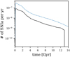 |
Fig. A.3. Same as Fig. 3, but for the IGIMF-R14-SD model. The SNIa events stop at about 13 Gyr because of the assumption that M2 > 0.8 M⊙, following Matteucci & Recchi (2001). |
All Tables
Input parameters and computation results of our best-fit chemical evolution models assuming the different IGIMF formulations introduced in Sect. 3.1 (lines 3 to 6) compared with the observational values (first line) and Lacchin et al. (2020) (second line).
All Figures
|
Fig. 1. SFHs. The SFH of the best-fit IGIMF-R14 model adopting the parameter set in Table 1 is shown with the black line. The SFH is shown as a histogram because the smallest time step is 10 Myr. The starting time of the galactic wind is 50 Myr (cf. Fig. 5), while the SFR drops to half of its peak value at about 90 Myr, which defines the SFT. The blue dashed line is the blue dashed line in Lacchin et al. (2020, their Fig. 3), i.e., their 3BooI-IGIMF model. |
| In the text | |
|
Fig. 2. Evolution history of the SNII rate. Similar to Fig. 1, but for the SNII rate of the best-fit IGIMF-R14 model. The initial spike SNII rate is due to the discontinuous 10 Myr time step where the metallicity increases from [Z] = − 7 to [Z] = − 4 at the second time step that leads to a sudden change in gwIMF according to the IGIMF-R14 formulation (see Fig. 4). The blue dashed line is the blue dashed line in Lacchin et al. (2020, their Fig. 5), i.e., their 3BooI-IGIMF model. |
| In the text | |
|
Fig. 3. Evolution history of the SNIa rate. Similar to Fig. 1, but for the SNIa rate of the best-fit IGIMF-R14 model. The blue dashed line is the blue dashed line in Lacchin et al. (2020, their Fig. 4), i.e., their 3BooI-IGIMF model. We note that the horizontal axis is different from Fig. 2. We also tested the DTD assumption of Lacchin et al. (2020) in our IGIMF-R14-SD model, shown in Fig. A.3. |
| In the text | |
|
Fig. 4. Cumulative (time-integrated) gwIMF (TIgwIMF) for all stars ever formed (thick solid line) and the gwIMF for each 10 Myr star formation epoch (thin solid lines, evolving from the top to the bottom as time progresses) of the best-fit IGIMF-R14 model, compared with the canonical IMF and the Salpeter IMF. We note that the gwIMF for the first epoch (the highest thin gwIMF line) has a significantly higher maximum stellar mass limit than the second epoch. This is only because the initial metallicity was assumed to be Z = 0.02 × 10⁻⁷ and because the 10 Myr time step is unresolved. |
| In the text | |
|
Fig. 5. Evolution of energy deposited in the gas by supernovae of the best-fit IGIMF-R14 model, compared to the (initial) nominal gas-binding energy assuming that the galactic radius and (phantom) dark matter mass does not evolve significantly (see Sect. 3.3). The galactic wind develops at the time step after the energy in gas exceeds the nominal binding energy. |
| In the text | |
|
Fig. 6. Mass evolution of gas, living stars, and stellar remnants of the best-fit IGIMF-R14 model. The gas mass stops to decrease at about 108.5 yr, when the star formation and the corresponding galaxy wind stops, and remains constant thereafter. The amount of remaining gas mass is discussed in Sect. 5. |
| In the text | |
|
Fig. 7. Evolution of [α/Fe]–[Fe/H] relations of the best-fit IGIMF-R14 model (black solid line). The circles are the data of Boötes I collected in Lacchin et al. (2020, their Fig. 6). The dashed line and the dash-dotted line are the two 3BooI models in Lacchin et al. (2020, their Fig. 6), assuming the gwIMF given by IGIMF-R14 and the Salpeter IMF, respectively. |
| In the text | |
|
Fig. 8. Stellar metal yield ratios of stars with different mass and metallicity given by Kobayashi et al. (2006). The yields from Kobayashi et al. (2006) for massive stars are connected to the yields for low- and intermediate-mass stars as given by Marigo (2001). The yields for M* > 40 M⊙ are the same as the yields for M* = 40 M⊙ stars. The red shaded region with log10(M*, initial[M⊙]) > 1.3073 indicates zero-metallicity stars with lifetimes shorter than 10 Myr, according to Yan et al. (2019). |
| In the text | |
|
Fig. 9. SFH requiring an artificial gas-cooling time. The blue dashed line is the same as in Fig. 1. Compared to the best-fit IGIMF-R14 model (with the SFH shown in Fig. 1), the discretised SFH has a larger spread but similar galaxy evolution results (see Sect. 7.5). |
| In the text | |
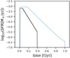 |
Fig. A.1. Same as Fig. 1, but for the IGIMF-R14-SD model. |
| In the text | |
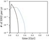 |
Fig. A.2. Same as Fig. 2, but for the IGIMF-R14-SD model. |
| In the text | |
|
Fig. A.3. Same as Fig. 3, but for the IGIMF-R14-SD model. The SNIa events stop at about 13 Gyr because of the assumption that M2 > 0.8 M⊙, following Matteucci & Recchi (2001). |
| In the text | |
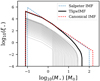 |
Fig. A.4. Same as Fig. 4, but for the IGIMF-R14-SD model. |
| In the text | |
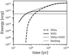 |
Fig. A.5. Same as Fig. 5, but for the IGIMF-R14-SD model. |
| In the text | |
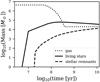 |
Fig. A.6. Same as Fig. 6, but for the IGIMF-R14-SD model. |
| In the text | |
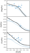 |
Fig. A.7. Same as Fig. 7, but for the IGIMF-R14-SD model. |
| In the text | |
Current usage metrics show cumulative count of Article Views (full-text article views including HTML views, PDF and ePub downloads, according to the available data) and Abstracts Views on Vision4Press platform.
Data correspond to usage on the plateform after 2015. The current usage metrics is available 48-96 hours after online publication and is updated daily on week days.
Initial download of the metrics may take a while.