| Issue |
A&A
Volume 637, May 2020
|
|
|---|---|---|
| Article Number | A61 | |
| Number of page(s) | 11 | |
| Section | Numerical methods and codes | |
| DOI | https://doi.org/10.1051/0004-6361/201936837 | |
| Published online | 14 May 2020 | |
Self-gravitating barotropic equilibrium configurations of rotating bodies with smoothed particle hydrodynamics
1
Departament de Física, Universitat Politècnica de Catalunya, EEBE, Eduard Maristany 16, 08019 Barcelona, Spain
e-mail: This email address is being protected from spambots. You need JavaScript enabled to view it.
2
Institut d’Estudis Espacials de Catalunya, Gran Capità 2-4, 08034 Barcelona, Spain
3
Departement Physik, Universität Basel, Klingelbergstrasse 82, 4056 Basel, Switzerland
e-mail: This email address is being protected from spambots. You need JavaScript enabled to view it.
4
Scientific Computing Core, sciCORE, Universität Basel, Klingelbergstrasse, 61, 4056 Basel, Switzerland
5
Department of Physics and Astronomy, University of Exeter, Exeter, UK
Received:
3
October
2019
Accepted:
21
March
2020
Abstract
Context. Self-gravitational rotating bodies do not have spherically symmetric geometries. The study of physical events appearing in fast-spinning compact stars and accretion disks, for example those due to localized thermonuclear ignitions in white dwarfs or to the role played by hydrodynamic instabilities in stars and disks, often requires 3D simulations. When the numerical simulations are carried out with the smoothed particle hydrodynamics (SPH) technique a critical point arises as to how to build a stable initial model with rotation because there is no well-established method for that purpose.
Aims. We want to provide a portable, easy-to-implement methodology for SPH simulations to procedurally generate physically sound, stable initial conditions for rotating bodies.
Methods. We explain and validate an easy and versatile novel relaxation method to obtain 3D equilibrium configurations of rotating bodies with SPH. As detailed below, this method is able to relax barotropic, P(ρ), structures either in rigid or differential rotation. The relaxation procedure strongly relies on the excellent conservation of angular momentum that characterizes the SPH technique.
Results. We applied our proposal to obtain stable rotating structures of single white dwarfs, compact binaries harboring two white dwarfs, high-density stars approached as polytropes and accretion disks either in rigid or differential rotation.
Conclusions. We present a novel relaxation method to build 3D rotating structures of barotropic bodies using the SPH technique. The method has been successfully applied to a variety of zero-temperature white dwarfs and polytropic self-gravitating structures. Our SPH results have been validated by comparing the main features (energies, central densities, and the polar-to-equatorial radius ratio) to those obtained with independent grid-based methods, for example, the self-consistent field method, showing that both methods agree within a few percent.
Key words: hydrodynamics / stars: rotation / methods: numerical / supernovae: general
© ESO 2020
1. Introduction
The smoothed particle hydrodynamics (SPH) technique has been widely used in astrophysics to study highly dynamical, geometrically distorted, and often catastrophic events, such as star formation (Springel & Hernquist 2003) and stellar encounters either from direct collisions (Lombardi et al. 1995) or with finite impact parameters (Davies et al. 1992). SPH has been used to model the gravitational radiation emission from the merging of white dwarfs (Lorén-Aguilar et al. 2005) and neutron stars (Rasio & Shapiro 1992). It has also been applied to simulate type Ia (García-Senz & Bravo 2005; Pakmor et al. 2012) and type II supernova explosions (Fryer & Warren 2002; Cabezón et al. 2018). It is also an important tool in the modeling of large-scale structure in the Universe (Springel 2005; Guedes et al. 2011).
Interestingly, the initial models in several of the scenarios above are simple barotropic configurations. In the particular case of the merging of two white dwarf (WD) stars, the final outcome could be a type Ia supernova (SNe Ia) explosion, being this double-degenerate scenario (DD) one of the favored production channels for these explosions (Hillebrandt et al. 2013). White dwarfs belonging to a compact binary system may have their rotational velocity substantially increased once the merger sets in, owing to the transfer of angular momentum from the accretion disk. Although it is thought that the accretion of matter from the companion star would lead to differential rotation (Yoon & Langer 2005), the assumption of rigid rotation is easy to implement and provides insight into many physical problems. Moreover, the rigid rotation hypothesis is adequate in those cases where the transport of angular momentum from the surface to the center of the star is very efficient (Piro 2008) as could be the case for degenerate objects like WDs. In particular, the fingerprint of the rotation in the thermonuclear explosion of a WD has been studied by Pfannes et al. (2010a,b) and García-Senz et al. (2018). In the latter, the SPH code SPHYNX (Cabezón et al. 2017) was used to simulate the explosion of a WD with mass ≃1 M⊙ in fast rigid rotation. In that calculation, the initial model was built using the relaxation scheme proposed in the present work. The models above belong to another SNe Ia explosion channel, which involves a single WD accreting mass from a companion, non-degenerate star through the Roche-Lobe overflow. This second possibility is called the single-degenerate scenario (SD) channel for SNe Ia. Both scenarios (DD and SD) involve large amounts of angular momentum, so the question arises of how to adequately model self-gravitating fast-spinning rotators with SPH.
Another topic where having good initial rotating models is crucial is the study of the interaction between the accretion disk around millisecond pulsars with their magnetospheres. Numerical simulations of these scenarios require the correct modeling of steady accretion disks, characterized by the total mass, angular momentum, and particular rotation law. Although there have been a number of works dealing with the interaction between accretion disk and magnetosphere (Parfrey & Tchekhovskoy 2017, and references therein) none of them was carried out with particle-based codes. Clearly, it would be very useful to have steady accretion disks with the adequate resolution to perform simulations of these scenarios with SPH.
Unfortunately, there is no general procedure to build initial conditions for such self-gravitational, rotating equilibrium structures with SPH. A mapping procedure from an axisymmetric grid of points to a 3D distribution of equal-mass SPH particles was briefly described in Durisen et al. (1986) in connection with the study of rapidly rotating n = 3/2 polytropes. Smith et al. (1996) used a similar mapping procedure to simulate the development of a dynamical bar instability in a spinning polytrope with n = 3/2. However, the direct mapping from grid-points to particles usually leads to incomplete equilibrium because the models presented in those works display excessive numerical noise1. A numerical scheme to handle disks in the presence of pressure gradients was discussed by Raskin & Owen (2016) and there are several recipes to approach the initial conditions prior to the dynamic merging of two WDs with SPH codes (Dan et al. 2011). There is, however, a rich literature concerning grid-based calculations of the equilibrium properties of barotropic, self-gravitating gases in rotation. An iterative algebraic method to obtain axisymmetric equilibrium structures is the self-consistent field (SCF) method developed by Ostriker & Mark (1968). Later, Hachisu (1986) successfully applied the SCF method to build zero-temperature spinning white dwarfs. Another approach was proposed by Eriguchi & Sugimoto (1981) in which the Poisson equation and the hydrostatic equilibrium equation (which includes the centrifugal force) are both used in integral form and iterated until convergence in a 2D grid of points. Nevertheless, these methods are not directly applicable to building initial models to carry out SPH calculations because the balance of gravity, pressure, and centrifugal forces is lost during the mapping procedure from the 2D ordered grid of points to a 3D distribution of particles.
As far as we know there is no public, well-documented, general procedure for obtaining self-gravitating structures in steady rotation with particle-based hydrodynamic codes. In this manuscript, we develop and test an easy yet practical novel relaxation scheme to build barotropic, P(ρ), 3D rotating structures in equilibrium under the SPH paradigm. In our proposal it is not necessary for the initial distribution of particles to match any prescribed SCF solution prior to relaxation. As an example, these relaxed structures can be used as suitable initial conditions to study the explosion of a rotating WD in the SD scenario, and as the outcome of the WDs merging in the DD scenario. In this work the relaxation scheme is applied to zero-temperature white dwarfs, to high-density polytropes, and to pseudo-Keplerian disks. To validate the method we provide quantitative comparisons with reference solutions, like those obtained by Hachisu (1986) and Eriguchi & Mueller (1985) using iterative time-independent methods such as the SCF scheme.
In Sect. 2 we describe the physical foundations of our proposal. Section 3 presents the application of the method to build 3D zero-temperature white dwarfs in rigid rotation. The scheme developed in Sect. 3 is also applied to the initial setting of two interacting WDs in a compact binary system in Sect. 4. The extension of the scheme to handle differential rotation in white dwarfs and polytropes is explained in Sect. 5. We apply the method to build pseudo-Keplerian accretion disks in equilibrium in Sect. 6. Finally, we present a summary of our findings and the prospects for future work in the conclusions in Sect. 7.
2. Relaxing rotating white dwarfs with SPH
In this section we aim to describe the physical basis of our relaxation scheme to obtain stable rotating structures of barotropic bodies, with particular emphasis in degenerate structures such as cold white dwarfs. Non-rotating equilibrium configurations of WDs can be obtained by relaxing a sample of particles with initial spherical coordinates (r, ϕ, θ). These SPH particles are radially distributed according to the density profile, but randomly in angles ϕ, θ. Usually, a damping force is added to the momentum equation so that after a few sound-crossing times the sample of particles relaxes to a stable configuration. It is worth noting, however, that as the mass of the WD approaches the Chandrasekhar-mass limit this equilibrium is not perfect and the degenerate star undergoes small radial oscillations. Fortunately, when simulating SNe Ia explosions the thermonuclear destruction of a massive WD is so fast that it is enough to keep the equilibrium only during a few sound-crossing times, tsc (typically tsc ∼ 0.46 s at ρ ≃ 109 g cm−3).
In the absence of rotation, the structure of the WD after the relaxation process is spherically symmetric and follows the well-known solution of the Lane-Emden (LE) equation. Thus, for an equation of state (EOS) dominated by a zero-temperature electron gas (Chandrasekhar 1939),
![Mathematical equation: $$ \begin{aligned}&P_{\rm e} =a\,[x(2x^2-3)(x^2+1)^\frac{1}{2}+3 {\sin h}^{-1} x], \end{aligned} $$](/articles/aa/full_html/2020/05/aa36837-19/aa36837-19-eq1.gif) (1)
(1)
 (2)
(2)
where a = 6.00 × 10²² dynes cm−2, b = 9.82 × 10⁵ μe g cm−3, and x is the Fermi momentum of electrons in relativistic units. The only parameters determining the density and pressure profiles are the mass of the WD and the electron molecular weight {MWD, μe}. Unfortunately, there is not a simple description that is equivalent to the Lane-Emden equation but for rotating stars. Assuming that the rotating white dwarf has axisymmetric geometry, its structure is set by the triad {MWD, JWD, μe} where JWD is its total angular momentum. For differential rotators it is necessary to additionally specify the rotational law followed by the angular velocity Ω(s), where s is the distance to the rotation axis.
Once these parameters are defined, the maximum density (ρmax) and radius (RWD) of the resulting configuration will be uniquely determined. It is important to note that the final values (ρmax and RWD) are different from those obtained when rotation is not present, even for the same combination of {MWD, μe}. Once the mass and its composition are fixed, a rotating WD will have a lower ρmax and larger RWD in the rotating plane than a non-rotating WD.
When studying the efficiency of nuclear burning in SNe Ia explosions, the dominant magnitude is the density. Therefore, we fix ρmax between rotating and non-rotating models which, as a consequence, implies a change in the total mass of the WD.
In this work, we consider the following rotation law:
 (3)
(3)
Here s is the distance to the rotation axis, Rc is a parameter that sets the size of the central core with nearly rigid rotation Ωc, and m is a parameter linked to the type of rotation (see Sects. 3 and 5). The current choices of m are m = 0 (rigid rotation), m = 1/2, and m = 1 (shellular). Rigid rotation is also attained for Rc ≫ RWD, independently of m.
Our relaxation method works as follows. First, we choose the values of ρmax, MWD, and JWD from Hachisu (1986) data tables (their Tables 4 and 5), and we take μe = 2 in the electron zero-temperature EOS. We then build an initial model with spherical symmetry (i.e., without rotation) and maximum density, ρmax. This model is obtained after integrating the Lane-Emden equation with inner boundary condition ρ(r = 0) = ρmax. We note that the total mass of the WD obtained from the LE equation,  , is not the same as the MWD of the rotating model in Hachisu’s tables for the same central density ρmax. The density profile is then mapped to a 3D distribution of equal-mass SPH particles, which ensures that the number density of the particles reflects the current density structure at any point. The mass of the particles is then re-scaled by a factor
  , so that the total mass becomes MWD. This changes the central density, but only transiently because its value is rapidly restored to ρmax during the relaxation process. Next, a velocity is given to each SPH particle so that the total angular momentum is JWD,
![Mathematical equation: $$ \begin{aligned} J_{\rm WD}=\sum _b m_b s_b { v}_b = \left[\sum _b m_b s_b^2 \left(1+\frac{s_b^2}{R_{\rm c}^2}\right)^{-m}\right]\Omega _{\rm c} (t), \end{aligned} $$](/articles/aa/full_html/2020/05/aa36837-19/aa36837-19-eq6.gif) (4)
(4)
from which the instantaneous value of Ωc(t) is obtained:
![Mathematical equation: $$ \begin{aligned} \Omega _{\rm c}(t) = \frac{J_{\rm WD}}{\left[\sum\nolimits _b m_b s_b^2\left(1+\frac{s_b^2}{R_{\rm c}^2}\right)^{-m}\right]}\cdot \end{aligned} $$](/articles/aa/full_html/2020/05/aa36837-19/aa36837-19-eq7.gif) (5)
(5)
It should be noted that when Rc → ∞ the angular velocity becomes Ω(t) = JWD/IWD(t), where IWD(t) is the time-dependent momentum of inertia of particles around the rotation axis, which is computed at each integration step during the relaxation. For other choices of Rc and m, Eq. (5) gives the correct angular velocity as a function of the generalized momentum of inertia of the system, provided JWD is known at t = 0. This original and simple recipe is physically sound and robust because it always preserves the total mass and total angular momentum of the system, even for highly deformed axisymmetric structures.
Once Ωc(t) is known, Eq. (3) gives Ω(s, t), so that the centripetal acceleration of each particle Ω × (Ω × r) is obtained. The particle distribution is henceforth relaxed in a co-moving reference frame. We then let the system freely evolve with the SPH code until equilibrium.
To relax the system and dissipate the spurious numerical noise stored in the velocity field the velocities are periodically set to zero (in the co-moving frame of reference). For example, all models in Table 1 with Np = 5 × 10⁵ particles were obtained by setting v = 0 every Δt ≃ tsc/3, being tsc the sound-crossing time (tsc ≃ 0.46 s in models with central density ρc = 109 g cm−3) until time t ≃ 5tsc/3. Afterwards the velocities were set to zero every Δt ≃ 0.8tsc s. Such simple recipe works well and can be adapted to handle different particle numbers and densities. After several sound crossing times, the final equilibrium configuration is attained and only a residual numerical noise remains. To decide when the particle distribution has converged to a stable, time-independent configuration, each calculated model has to fulfill two criteria: that its central density and equatorial radius become constant (except small oscillations with amplitude 1–2% around their average value), and that the oscillations around the average value of the central density, the polar and equatorial radius, and the total kinetic, internal and gravitational energies remain lower than ≃2% when the system is left free to evolve in the current inertial frame (i.e., without re-setting the velocities to zero).
3. Isolated WDs with rigid rotation
As a first application we focus on the evolution towards equilibrium of models calculated assuming rigid rotation for both single WDs and double-degenerate stars in compact binaries. Some insights into how to handle differential rotation while obeying the rotation law given by Eq. (3) with m ≠ 0 are provided in Sect. 5. The simulations presented here, were carried out with the hydrodynamic code SPHYNX, using the electron zero-temperature EOS given by Eq. (1) with μe = 2. The calculations were performed with the default values of several parameters, for example α = 4/3 in the artificial viscosity (AV), with the Balsara limiters (Balsara 1995) to the AV turned on. The gravitational force is approached by a multipole expansion up to quadrupole terms, with the tolerance parameter θ (Hernquist 1987), set to θ = 0.6. An exponent parameter, p (0 ≤ p ≤ 1), allows choosing among different volume elements (VEs; Cabezón et al. 2017). The present simulations were obtained with p = 0, which is equivalent to the common choice VE = m/ρ.
A cautionary remark concerning rigid fast rotation close to Keplerian values is necessary here. For these models we observed that the combination of solid rigid rotation and a high rotational speed led to a harmful feedback between the centrifugal, gravitational, and pressure forces at the equator surface. Let us assume that there is a particle with a slight excess of angular velocity which displaces it farther in radius, thus increasing the centrifugal force (but weakening the gravity). This particle will move farther out, which again increases the centrifugal force, and so on. Even if a similar feedback only affects a handful of surface particles located on the equator, it is enough to spoil the convergence. If we want to make quantitative comparisons between our results and those by the SCF method for perfect rigid rotators, a solution is to (artificially) reduce a bit the gradient of pressure at the surface so that the feedback above is broken, even in the presence of low amounts of numerical noise. A simple way to do this while keeping the relaxation stable is to reduce the pressure in the low-density regions of the WDs by multiplying the electron pressure, Eq. (1), by a density cutoff:
 (6)
(6)
Here P is the pressure used in the calculations and ρcrit = αρmax, being ρmax the maximum density, which in the models shown in Table 1 is attained at the center of the configuration. We empirically found that α = 5 × 10⁻⁴ works well in almost all the rigidly rotating models shown in Table 1. Slightly lower values, α = 2.5 × 10⁻⁴ and α = 2 × 10⁻⁴, were used to relax the more massive models A21 and A22, to reduce the error in the equatorial radius. Other magnitudes, such as the central density and total kinetic, internal, and gravitational energies, are rather insensitive to the precise value of α. We note again that this density cutoff is merely a way to facilitate the convergence of the relaxation. It affects a negligible amount of mass, and makes it possible to perform a direct comparison with the results obtained with the SCF method for rigid rotators. In real calculations, however, it is preferable not to consider absolute rigid rotation and to allow for some amount of differential rotation at the external layers. In this case, introducing the above density cutoff becomes unnecessary.
Here we carry out the relaxation of several WDs with different {MWD, JWD}. An estimation of the accuracy of the resulting equilibrium configurations is done by comparing our results to those of Hachisu (1986), which were obtained using the SCF method.
We provide a representative example of the evolution towards equilibrium of one of our rotating models in the left panel of Fig. 1, which depicts the evolution of the central density ρc (ρc = ρmax in these models), equatorial radius, Req, and angular velocity, Ω. As we can see, the central density and angular velocity evolve in a similar manner. They start from relatively high values, decrease fast over a few tenths of a second, and stabilize at t ≃ 1 s. The equatorial radius follows the opposite trend: it is low at the beginning, then it rises quickly to asymptotically stabilize at t ≃ 2.0 s. From Fig. 1 it is obvious that the characteristic relaxation times of ρc and Req are quite different. To check that the star was stable we stop resetting the velocities to zero at t = 2.5 s, so that the system evolves freely in the current inertial frame of reference. The only source of dissipation being the artificial viscosity (AV) term, as given by Monaghan (1997), including the Balsara limiters. As can be seen, the central density remained stable during at least Δt ≃ 3 s (≃7 times the sound-crossing time). We show a color map slice of the density of model A21 at t = 2.5 s in Fig. 1 (right). The white dwarf is neatly oblated with a polar-to-equator radius  which is ≃7.3% larger than that given by the SCF method. This is, however, the largest discrepancy found across all the calculated models in Table 1. The differences with respect the results by Hachisu remain, for the most part, below 4%.
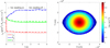 |
Fig. 1. Simulation results of models A21 and A22 in Table 1. Left: evolution of central density (in 109 g cm−3), radius (in 108 cm), and angular velocity Ω. Solid lines correspond to model A21 (5 × 10⁵ particles) and dashed lines to model A22 (2 × 10⁶ particles). Once the periodic resetting to zero of the velocities is removed at t = 2.5 s, the central density remains stable during several sound-crossing times (tsc ≃ 0.4 s). Right: density color map and isodensity contours of a 2D meridional slice of the rotating WD at t = 2.5 s. The slice has a thickness of four times the local smoothing length (4 h), which represents roughly 10% of the total number of particles. Making cuts with the local value of h ensures a similar number of particles at any region of the color map. |
Table 1 summarizes the relevant information of the calculated models. Models A refer to the SPHYNX calculations and H refer to the SCF models by Hachisu. Models A1 and H1 are non-rotating, with a mass close to the Chandrasekhar-mass limit. As we can see, the fit is excellent. The larger discrepancy, ≃4%, is in the radius of the configuration. Actually, this is something we expected because a white dwarf nearing the Chandrasekhar-mass limit does not have a well-defined scale length. We thus expect that the larger differences with respect the SCF method affect the equatorial radius and the oblateness of the WDs at central densities ρ9 ≥ 1. Model A22 in Table 1 is the same as A21, but calculated with four times more particles. It leads to a stable model with similar relative errors in the central density, equatorial-to-polar radius and total energies, with respect to those of the reference model H2. Therefore, our relaxation method is able to match the results by Hachisu in a wide range of stellar masses, 0.67 M⊙ ≤ MWD ≤ 1.44 M⊙. The lower mass is close to that of a standard WD and the higher mass is actually at the Chandrasekhar-mass limit of a non-rotating white dwarf. The case of a super-Chandrasekhar-mass white dwarf stabilized by rotation is discussed in Sect. 5.2.
4. WDs in a double-degenerate binary system
A straightforward and timely extension of the relaxation procedure described above can be used to generate suitable initial models to study the DD production channel for SNe Ia. In the DD channel two WDs, settled in a compact orbit, move closer because of gravitational-wave radiative losses. At some point the gravitational pulling from the more massive WD breaks the lighter compact star and an accretion disk around the surviving WD forms. The further accretion of the debris would eventually provoke the explosion of the initially more massive white dwarf (Hillebrandt et al. 2013).
A key technical point of the simulations of the DD scenario is how to set the initial conditions immediately prior to the merging. The currently accepted standard procedure involves a two-step process (Rosswog et al. 2004; Dan et al. 2011). First, both stars are relaxed in isolation. Then, both stars are placed in a wide enough binary orbit in order to prevent any immediate mass transfer episodes. Subsequently, the binary system is evolved in the co-rotating frame where an artificial acceleration term is introduced in order to continuously shrink the orbital distance between the two white dwarfs. The orbital distance will be decreased at a sufficiently slow rate so the stars remain relaxed at all times, and so they slowly and continuously deform without introducing any spurious oscillations. The relaxation process will be finished when the secondary star starts to overflow its Roche lobe. This method is, however, computationally expensive and somewhat artificial because both WDs need to be relaxed all the time along the path from the initially detached position until they reach the onset of the merger (usually achieved through the introduction of additional artificial dissipative terms).
A somewhat more elegant and fast procedure is to relax both stars taking into account their angular momentum once they are already settled in a close orbit just prior to the merging, thus avoiding the intermediate relaxation stages. To do this we first set the orbit parameters so that the gravitational pulling onto the surface of the less massive WD becomes a sizable fraction (β) of its own gravity. That constraint leads to the following expression for the distance:
 (7)
(7)
Here MWD1 and MWD2 are the masses of the more massive and lighter components, respectively. Once D1, 2 is known, and assuming a circular orbit, we calculate the velocity of the center of mass of each star with respect to an inertial reference frame located at rest at the center of mass of the binary system. The total angular momentum of the binary system Jsys is calculated afterwards so that we can benefit from the scheme developed above in Sects. 2 and 3.
As an example, we have calculated the stable initial configurations in two cases. We first consider a system of twin white dwarfs with canonical masses MWD1 = MWD2 = 0.606 M⊙ and parameter β = 1/4. The second case is for MWD1 = 0.796 M⊙, MWD2 = 0.606 M⊙, and the same value of β. The center of the compact stars is supposed to move in circles around the center of mass of the binary system, with angular velocity Ω. The total angular momentum of the system is Jsys = Jorb + Jspin. In this work we focus on pairs of white dwarfs which are tidally locked so that Ωspin = Ωorb = Ω. Therefore, once Ω is deduced from
 (8)
(8)
the total angular momentum Jsys = Jorb + Jspin is easily obtained2. The post-relaxed binary configuration in rigid rotation will be determined by {MWD1, MWD2, Jsys}. The EOS was that of a zero-temperature electron gas given by Eq. (1). A summary of the parameters used in these simulations is given in Table 2.
Main features of the double-degenerate models.
The evolution of the central densities of both WDs in model DD2 is shown in Fig. 2 (left). The initial values of central density for both stars are considerably higher at the beginning of the relaxation process, as expected from spherically symmetric initial models. As the simulation proceeds the system rapidly achieves a stable configuration with lower densities due to the influence of rotational effects and tidal forces and to the re-ordering of the particles. This stable configuration is reached very quickly (∼1 s for the more massive star and ∼5 s for the other). At t = 20 the periodic reset to zero of the velocities was turned off without any appreciable effect on the evolution of the two stars. We also provide the equilibrium configuration of the WDs in the same figure (right panel), obtained in the co-moving non-inertial frame of reference located at the center of mass. Each dot represents an SPH particle within a thin cut along the plane Z = 0. The color-coding shows the logarithm of density. Comparing the two snapshots, it is clear that the initially spherical random particle distribution reaches a more ordered distribution where the least massive star is asymmetrically elongated in the direction of the more massive, as expected. After the relaxation we checked that the final structure remains stable during at least one complete orbit in the inertial frame. Although the final binary configuration is stable, it is on the verge of Roche-lobe overflow. To trigger the catastrophic merging of the WDs it is enough to slightly shrink the distance D1, 2.
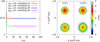 |
Fig. 2. Initial setting of the DD scenario. Left: evolution of the central density of both WDs during the relaxation (t ≤ 20 s) and the free evolving (t ≥ 20 s) stages. The orbital period is P ≃ 70 s. Right: slice in the orbital plane depicting the density color map of each white dwarf at t = 0 s (initial spherically symmetric configuration) and t = 20 s (final relaxed model). The slice has a thickness of four times the local smoothing length value (4 h). The center of mass of both configurations is located at (0, 0) km, but the snapshots have been shifted 14 000 km to the left and to the right to avoid the superposition of the images. |
5. Differential rotation
It is feasible to apply the proposed relaxation method to handle differential rotation. We analyze here the impact of taking m ≠ 0 in Eq. (3) with different values of the parameter Rc. We first discuss the case of rotating polytropes of index n = 3/2 with central densities and sizes close to those characterizing neutron stars (NSs). The case of a zero-temperature rotating white dwarf with differential rotation is discussed later. In all cases the results were checked with well-known existing solutions obtained via other independent methods.
5.1. Case 1: differentially rotating high-density polytropes
To check the ability, as well as the limits, of our relaxation scheme to handle non-rigid rotation we chose a polytropic relation
 (9)
(9)
with γ = 5/3. In a non-rotating model this value produces a very stable spherically symmetric object whose structure is obtained after solving the Lane-Endem equation with n = 1/(γ −1) = 3/2.
Our initial pre-relaxed model is a spherically symmetric object with mass M = 2 M⊙ and central density ρc = 1014 g cm−3. This combination sets the polytropic constant in Eq. (9) to K = 1.72 × 10¹⁰. The integration of the LE equation leads to an object of radius RNS ≃ 38 km, roughly compatible with a NS size. Some amount of total angular momentum J was then added to the polytrope and the structure relaxed with the method explained in Sect. 2. The angular momentum J was chosen so that the square of the dimensionless angular momentum j,
 (10)
(10)
matches the values in Tables 1 and 2 in Eriguchi & Mueller (1985, hereafter EM) so that meaningful comparisons with their results can be made. We note, however, that the value of ρmax in Eq. (10) initially differs from that in EM because we take ρmax = ρc of the spherically symmetric polytrope, instead of the maximum density of the rotating structure used by EM. This initial choice of ρmax is motivated by the fact that we do not know the true value of the density of the rotating structure prior to relaxation. Nevertheless, this does not pose a problem because the value of j can be recalculated with the value of ρmax obtained once the relaxation has ended. This new value of j (Col. 6 in Table 3) was the one used to check our results with those given in the EM tables.
Main features of the relaxed high-density rotating polytropes (ρmax = 1014 g cm−3 prior to relaxation) calculated with γ = 5/3 and mass M = 2 M⊙.
We calculated three models using j-constant (m = 1) and two more with v-constant (m = 1/2) rotational laws. In each case we consider Rc = ARNS with A = 2 and A = 0.2 in Eq. (3), respectively. The case A = 2 is actually close to rigid rotation, but the case A = 0.2 is representative of models with large differential rotation. Table 3 shows a summary of the results, where the meaning of the columns is as follows: J (Col. 4) is the total angular momentum; ρmax is the maximum density of the rotating body (not necessarily achieved at the center); Ek, EI, and EG is the total kinetic, internal, and gravitational energy, respectively; and E0 is a normalization energy defined by
 (11)
(11)
The symbol V.T refers to the virial theorem defined as V.T =|(2Ek + EG + 3(γ −1)EI)/EG|, Ωc is the angular velocity at the center of the polytrope and, finally, F = Rp/Req is the polar-to-equatorial radius.
As shown in Table 3, the global energies and the polar-to-equator ratio agree with the results by EM within a few percentage points. Nevertheless, models Bn do not fulfill the virial theorem as well as they do in the EMn calculations. There is almost a factor of ten difference between the two estimations. This discrepancy arises from the very different approach to the structure equilibrium of the rotating polytropes. In the case of the SPH calculation the equilibrium is approached dynamically in full 3D, while in the EM calculation the equilibrium equations are solved by means of a time-independent iterative procedure in a fixed 2D grid of points.
Figure 3 depicts the evolution of ρmax (left panel) and Ωc (right panel) for several of the models in Table 3. The profiles are similar to those shown in Fig. 1 of an isolated rotating white dwarf, but with a temporal scale of milliseconds instead of seconds. The final equilibrium value of Ωc oscillates slightly around a stable value that, depending on the model, is in the range 103 s−1 ≤ Ωc ≤ 104 s−1. This corresponds to periods of 0.6 ms ≤P ≤ 6 ms, typical of millisecond pulsars. Figure 4 shows several density color maps along meridional slices of models Bn. The first column depicts the color maps of pseudo-rigid rotators (A = 2), being the case m = 1 (model B1) less elongated than m = 1/2 (model B4). According to EM, this last case is very close to the critical value, Rp/Req = 0.5988, at which the gravitational and centrifugal forces become equal at the surface of the configuration when the rotation is 100% rigid (Eriguchi & Mueller 1985).
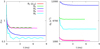 |
Fig. 3. Approach to the equilibrium of models described in Table 3 as a function of time: density (left panel) and Ωc (right panel). |
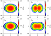 |
Fig. 4. Color map of density in a meridional cut (with thickness 4h and axis units in km) of several models, as described in Table 3. |
Models B3 and B5 (A = 0.2) host a strong differential rotation and become highly deformed, with ρmax achieved far from the geometrical center of the configuration (see Fig. 4, right column). In particular, model B3 is close to the limiting configuration at which our relaxation method gives satisfactory results when the trial initial configuration (prior to relaxation) is a spherically symmetric LE model. This occurs because of the large contrast between the angular velocity at the center and at the surface equator, which in model B3 is Ωc/Ωeq ≃ 40. Obtaining suitable models for much higher angular velocity ratios would require a more refined trial initial configuration, for instance those obtained with the SCF method, and increased resolution, which is left for a future work.
5.2. Case 2: isolated WD with differential rotation
We consider again a spinning zero-temperature white dwarf, but this time with differential rotation. In particular, we focus on initial models obeying the rotation law given by Eq. (3) and m = 1/2. This choice leads to rigid rotation at the center (s ≤ Rc) of the configuration, but becomes Keplerian at distances s ≫ Rc. As previously stated, the case m = 1/2 is usually referred to as v-constant in the literature. As can be seen in models A6, 7 in Table 1, we find a good agreement between our models and those reported by Hachisu for the case m = 1/2 (models H6, 7 in Table 1). For these models Rc = 0.1 Req, where the value of Req was taken from the work by Hachisu (models 3 and 4 with ρmax = 109 g cm−3 in their Table 4). Another example of differential rotation, with an exponent intermediate between m = 1/2 and m = 1, is discussed in the following section.
We show a summary of our results for the two cases with m = 1/2 in Table 1 and Fig. 5. The two models differ from the SCF calculations by less than 5%, being stable enough for further hydrodynamic calculations. Figure 5 (left), shows the evolution of the maximum density and central value of the angular velocity for model A7. At t ≃ 1 s the magnitudes ρmax and Ωc both become stable. The profile of the angular velocity Ω has been superposed on the density color map (right). It is clear that the maximum density is not located at the center of mass of the configuration, which is a typical signature of models with high angular momentum. The value of the angular velocity Ω is maximum at the center of the configuration and is very high, Ω(s = 0) ≃ 18 s−1.
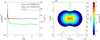 |
Fig. 5. Time evolution of the maximum density and central angular velocity in model A7, with differential rotation (left). Superposed on the density color map, with thickness 4h, is the 1D profile of angular velocity (green) along a 1D cut on the equator plane (right). |
After being relaxed, the rotating white dwarf is allowed to evolve freely during ≃10 complete orbits of the fastest particle. During that time the central density remains constant (left panel in Fig. 5), while the central angular velocity Ωc slightly oscillates around 18.4 s−1. What is shown in Fig. 5 at t > 1.2 s is the average value of Ωc for all particles with s ≥ 3 × 106 cm. An estimate of Ωc(sa) is obtained from the tangential velocity of particle a, vt(sa, t) through Eq. (3):
 (12)
(12)
6. Pseudo-Keplerian disks orbiting a central mass-point
Steady rotating disks are a universal phenomena in astrophysics (e.g., Frank et al. 2002) and often appear in merging stellar binary systems and during stellar and planetary formation (Armitage 2011). Because of the thermal pressure contribution, these disks cannot be described in a purely Keplerian way. Pressure gradient effects are important and have to be taken into account to adequately model the structure of steady or pseudo-steady disks. Nevertheless, the simulation of pressure supported accretion disks with any hydrodynamic method has been proven difficult, especially when keeping track of the structure during many orbital periods. In the particular case of SPH codes, there is an extra difficulty in building a stable enough initial distribution of particles with pressure gradients in differential rotation (Owen 2004).
With the aim of checking the abilities of our relaxation scheme, we have implemented the generalized disk test problem discussed by Raskin & Owen (2016). An idealized disk was assumed to have cylindrical geometry and can be studied in 2D. As shown by these authors, the gravitational potential ϕ(r), pressure (P(r) = Kργ, with γ = 3/2), density, and tangential velocity (vθ) profiles follow precise analytic relationships, which we reproduce here for completeness:
 (13)
(13)
![Mathematical equation: $$ \begin{aligned}&\rho (r) =\left[\frac{\mathrm{GM}(\gamma -1)}{K\gamma (r^2+r_s^2)^\frac{1}{2}}\right]^{\frac{1}{(\gamma -1}}\cdot \end{aligned} $$](/articles/aa/full_html/2020/05/aa36837-19/aa36837-19-eq18.gif) (14)
(14)
The expressions above correspond to a pressure-supported disk with zero angular momentum. To introduce rotation, a reduction factor fp in the pressure is assumed so that the EOS is P(r) = Kργ fp. To keep the equilibrium, the loss in the pressure-gradient force is compensated by adding a centripetal force created by a tangential velocity field,
 (15)
(15)
For this test we set GM = 1, rs = 0.5, and fp = 0.5. The value of K in the EOS is obtained from Eq. (14), assuming ρ(r = 0) = ρ0 = 1, giving K = 2/3. The resulting disk is pseudo-Keplerian with an important contribution of pressure. Finally, we want to study both the resulting profiles of our relaxed initial models and the ability of SPHYNX to keep the disk in steady rotation during many orbits.
Because it is a 2D calculation, it is feasible to build an initial model by spreading the particles in an ordered array according to the density profile (Eq. (14)). As shown by Owen et al. (1998) and Raskin & Owen (2016), it is enough to distribute the particles in rings so that the radial separation between particles is adjusted in each annulus such that the angular separation between particles at a given radial coordinate is constant. In this work we propose a different procedure, which is capable of generating good initial models, but with glass-like structure.
First, we fit the angular velocity Ω(r) = vθ(r)/r obtained from Eq. (15) with good accuracy, by the rotation law given by Eq. (3) with Ωc(t = 0) = 2, m = 0.730, and rc = 0.478. The total angular momentum of the disk, JD, is estimated from the fitted Ω(r) and ρ(r), with 0 ≤ r ≤ RD, where RD = 10 is the adopted disk radius. The main features of our initial model are summarized in Table 4. A sample of N = 9 × 10⁴ particles3 was radially distributed in a plane according to the density profile, while their angular position 0 ≤ θ ≤ 2π is set at random. Afterwards, the particle sample is relaxed with the procedure described in Sect. 2.
Main features of the disk model after being relaxed: mass, angular momentum, and rotation constants Ωc [s−1].
Figure 6 shows the density, pressure, and tangential velocity profiles of the particles once the relaxation has ended (t = 0 cases). A density color map showing the central region of the disk with r ≤ 3 is depicted in the left semi-plane of the bottom right panel in the same figure. In spite of the disordered glass-like pattern, the distribution of the SPH-particles in the disk matches the analytic profile very well. Furthermore, after the relaxation, this pseudo-Keplerian disk should retain its structure during as many orbits as possible. It was shown by Raskin & Owen (2016) that many current SPH schemes fail to preserve the disk features after about a dozen periods of the particle at maximum velocity. Satisfactory results were obtained with the conservative reproducing kernel (CRKSPH) method by Frontiere et al. (2017) in combination with the AV switches by Cullen & Dehnen (2010).
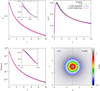 |
Fig. 6. Profiles of density, tangential velocity, and pressure of the disk after the relaxation period (green lines) compared to the analytic values (in red) and after t = 200 s calculated with the Balsara limiter (blue) or the AV switches by Read & Hayfield (2012) (magenta). Bottom right panel: density color map in the central region of the disk. The left semi-plane (x < 0) is for the relaxed model at t = 0 s; the right semi-plane (x ≥ 0) shows the density color map after t = 200 s, with the Balsara limiter. Unlike in Raskin & Owen (2016), the SPH particles are still settled in a glass-like configuration. |
The stability of the disk obtained with our relaxation scheme was further checked with the SPHYNX code. We want to know if the integral approach to the gradients in combination with either the Balsara limiter (Balsara 1995) or the AV switches (Cullen & Dehnen 2010; Read & Hayfield 2012) is capable of keeping the disk in steady state over many orbital periods. For this calculation the EOS was changed to P = (γ −1)ρu (γ = 5/3), where u is the specific internal energy of the gas. The evolution of the internal energy was obtained by evolving the corresponding energy equation.
We have tracked the evolution until t = 200 s, so that the results can be compared to those obtained by Raskin & Owen (2016) with the CRKSPH method. At t = 200 s the particle with the highest velocity has completed ≃40 orbits around the center of the disk. As shown in Fig. 6, the deviation of ρ(s),vt(s), and P(s) from either the analytic or the t = 0 s profile is very small. Particularly good is the fit of the tangential velocity, which still matches the initial profile after ≃40 orbits. Nevertheless, a closer look into the density profile in the central region indicates that its value is slowly growing with time. We agree with Raskin & Owen (2016), that such small growth of the central density is an artifact of the particular implementation of the artificial viscosity. It is slightly less pronounced when the switches to the AV are in command of the dissipation. It is worth noting, however, that the pressure profile remains very close to the analytic value.
The x ≥ 0 semi-plane in the bottom right panel in Fig. 6 depicts the density color map at t = 200 s in the central part of the disk. As we can see, the differences with the color map at t = 0 s (x < 0 semi-plane) are small, being only relevant at the very center of the configuration. Additionally, the model still retains a good glass-like granulation, with no indications of pairing instability after ≃40 revolutions.
7. Conclusions
A common problem in simulating the evolution of compact objects with SPH is that there is not a general procedure to obtain stable initial models when these objects are spinning quickly. In this paper we propose and test an easy and versatile relaxation scheme for building stable rotating models of self-gravitating bodies whose EOS is of barotropic type. The hypothesis of barotropic EOS allows to handle many interesting objects such as isothermal white dwarfs, neutron stars, and polytropic structures. As detailed in Sect. 2, our method relies on the exceptional angular momentum conservation properties of the SPH technique.
We apply our method to get stable rotating configurations of zero-temperature WDs with different masses and total angular momentum. We were able to build stable models of rotating white dwarfs and polytropes spanning a wide mass range, 0.67 M⊙ ≤ MWD ≤ 2 M⊙, with both rigid and differential rotation. The main magnitudes (central density; total kinetic, internal, and gravitational energies; equatorial and polar radius) match the semi-analytical results by Hachisu (1986) and Eriguchi & Mueller (1985), in general within a few percentage points. Given the current uncertainties in the particular rotation law followed by these compact objects, this precision is enough to explore many issues concerning their evolution, either for explosion or collapse scenarios. Additionally, we show that our method is able to produce stable configurations when it is applied to a pair of white dwarfs orbiting in a compact binary system. This last scenario is of capital importance to understanding the double-degenerate route to SNe Ia explosions.
Finally, we have applied the method to produce a steady accretion disk with cylindrical symmetry. Even though the assumption of cylindrical geometry is not realistic, this configuration has the advantage that it has an analytical solution for comparison, while still retaining many of the features of real disks. The ensuing relaxed disk is characterized by a glass-like distribution of particles in differential rotation, partially supported by pressure effects and by rotation. As shown in Sect. 6, this pseudo-Keplerian disk is in a good steady state, being stable over several dozen orbits of the particle at maximum velocity.
Presently, two cautionary remarks have to be taken into account before applying our procedure to astrophysical calculations. First, the centrifugal force has to remain weaker than the gravitational pull at the equator when approaching the equilibrium configuration. Otherwise a harmful tradeoff between gravity (∝1/s2) and the centrifugal force (∝s) may appear which finally leads to the ejection of particles located in the outer shells along the equatorial plane. Second, in differential rotation the ratio of the angular velocity at the center to that at the surface, prior to relaxation, should be not too extreme. In particular, the combination of a shellular (m ≃ 1) rotation with a high total angular momentum and low values of Rc in Eqs. (3) and (5) lead to toroidal structures where rp/req → 0 (Eriguchi & Mueller 1985). Difficulties may also appear when trying to relax bodies with extremely large density contrasts between the core and the surface layers, owing to their very different characteristic timescales. In these cases, the choice of spherically symmetric Lane-Endem models as initial trial configurations is not adequate because they are too far from the final equilibrium structure and the relaxation to a steady state could be hard or even impossible. This difficulty can probably be overcome using better initial trial models, for example those obtained with the SCF method or even envisaging the final toroidal structure as the result of the coalescence of two spherically symmetric objects (as was done in Sect. 4).
The practical cases studied in this work cover only a small subset of the potential applications. An immediate additional application of our method may consist in building 3D stable post-Newtonian models of fast-rotating neutron stars, either isolated or in binary systems. This task should not be difficult because the EOS of cold neutron stars can also be described assuming zero temperature.
Prospects for future extensions of this work may include the impact of finite temperature gradients in the relaxed rotating structures. Currently, the steady spinning polytropes obtained in Sect. 5.1 with a barotropic EOS, P = Kργ, can be easily mapped into an axisymmetric distribution of temperature if we assume a realistic EOS, P(ρ, T), i.e., that of a non-degenerate ideal gas. This suggests that relaxing a trial initial model with a realistic EOS besides a superimposed axisymmetric temperature profile, T(s), from the onset is feasible.
Nevertheless, the large amount of numerical noise present in the initial models was used by the authors of these works as the seeds of several rotational induced instabilities.
This is not the only way to make a reasonable guess of Jsys before relaxation. Another possibility is to use the modified Kepler’s law (Lai et al. 1994), which is the result of considering deformed ellipsoids. What is relevant, however, is that once it has converged the DD system has a structure compatible with the initial choice of Jsys.
This particle count, spread in a disk radius RD = 10, is equivalent to the N = 7800 particles and RD = 3 adopted in Raskin & Owen (2016), so that the comparison is meaningful.
Acknowledgments
This work has been supported by the MINECO Spanish project AYA2017-86274-P and the Generalitat of Catalonia SGR-661/2017 (DG), and by the Swiss Platform for Advanced Scientific Computing (PASC) project SPH-EXA: Optimizing Smooth Particle Hydrodynamics for Exascale Computing (RC and DG). JMBI acknowledges the support by the FPU fellowship and wants to thank the Ministerio de Educación, Cultura y Deporte from Spain. The authors acknowledge the support of sciCORE (http://scicore.unibas.ch/) scientific computing core facility at University of Basel, where part of these calculations were performed.
References
- Armitage, P. J. 2011, ARA&A, 49, 195 [NASA ADS] [CrossRef] [EDP Sciences] [Google Scholar]
- Balsara, D. S. 1995, J. Comput. Phys., 121, 357 [NASA ADS] [CrossRef] [Google Scholar]
- Cabezón, R. M., García-Senz, D., & Figueira, J. 2017, A&A, 606, A78 [NASA ADS] [CrossRef] [EDP Sciences] [Google Scholar]
- Cabezón, R. M., Pan, K.-C., Liebendörfer, M., et al. 2018, A&A, 619, A118 [NASA ADS] [CrossRef] [EDP Sciences] [Google Scholar]
- Chandrasekhar, S. 1939, An Introduction to the Study of Stellar Structure (Chicago: University of Chicago Press) [Google Scholar]
- Cullen, L., & Dehnen, W. 2010, MNRAS, 408, 669 [NASA ADS] [CrossRef] [Google Scholar]
- Dan, M., Rosswog, S., Guillochon, J., & Ramirez-Ruiz, E. 2011, ApJ, 737, 89 [NASA ADS] [CrossRef] [Google Scholar]
- Davies, M. B., Benz, W., & Hills, J. G. 1992, ApJ, 401, 246 [NASA ADS] [CrossRef] [Google Scholar]
- Durisen, R. H., Gingold, R. A., Tohline, J. E., & Boss, A. P. 1986, ApJ, 305, 281 [CrossRef] [Google Scholar]
- Eriguchi, Y., & Sugimoto, D. 1981, Prog. Theor. Phys., 65, 1870 [NASA ADS] [CrossRef] [Google Scholar]
- Eriguchi, Y., & Mueller, E. 1985, A&A, 146, 260 [NASA ADS] [Google Scholar]
- Frank, J., King, A., & Raine, D. J. 2002, Accretion Power in Astrophysics: Third Edition (Cambridge: Cambridge University Press) [Google Scholar]
- Frontiere, N., Raskin, C. D., & Owen, J. M. 2017, J. Comput. Phys., 332, 160 [NASA ADS] [CrossRef] [Google Scholar]
- Fryer, C. L., & Warren, M. S. 2002, ApJ, 574, L65 [NASA ADS] [CrossRef] [Google Scholar]
- García-Senz, D., & Bravo, E. 2005, A&A, 430, 585 [NASA ADS] [CrossRef] [EDP Sciences] [Google Scholar]
- García-Senz, D., Cabezón, R. M., & Domínguez, I. 2018, ApJ, 862, 27 [NASA ADS] [CrossRef] [Google Scholar]
- Guedes, J., Callegari, S., Madau, P., & Mayer, L. 2011, ApJ, 742, 76 [NASA ADS] [CrossRef] [MathSciNet] [Google Scholar]
- Hachisu, I. 1986, ApJS, 61, 479 [NASA ADS] [CrossRef] [Google Scholar]
- Hernquist, L. 1987, ApJS, 64, 715 [NASA ADS] [CrossRef] [Google Scholar]
- Hillebrandt, W., Kromer, M., Röpke, F. K., & Ruiter, A. J. 2013, Front. Phys., 8, 116 [Google Scholar]
- Lai, D., Rasio, F. A., & Shapiro, S. L. 1994, ApJ, 420, 811 [NASA ADS] [CrossRef] [Google Scholar]
- Lombardi, J. C. Jr, Rasio, F. A., & Shapiro, S. L. 1995, ApJ, 445, L117 [NASA ADS] [CrossRef] [Google Scholar]
- Lorén-Aguilar, P., Guerrero, J., Isern, J., Lobo, J. A., & García-Berro, E. 2005, MNRAS, 356, 627 [NASA ADS] [CrossRef] [Google Scholar]
- Monaghan, J. J. 1997, J. Comput. Phys., 136, 298 [NASA ADS] [CrossRef] [MathSciNet] [Google Scholar]
- Ostriker, J. P., & Mark, J. W. K. 1968, ApJ, 151, 1075 [NASA ADS] [CrossRef] [Google Scholar]
- Owen, J. M. 2004, J. Comput. Phys., 201, 601 [NASA ADS] [CrossRef] [Google Scholar]
- Owen, J. M., Villumsen, J. V., Shapiro, P. R., & Martel, H. 1998, ApJS, 116, 155 [NASA ADS] [CrossRef] [Google Scholar]
- Pakmor, R., Kromer, M., Taubenberger, S., et al. 2012, ApJ, 747, L10 [Google Scholar]
- Parfrey, K., & Tchekhovskoy, A. 2017, ApJ, 851, L34 [NASA ADS] [CrossRef] [Google Scholar]
- Pfannes, J. M. M., Niemeyer, J. C., & Schmidt, W. 2010a, A&A, 509, A75 [NASA ADS] [CrossRef] [EDP Sciences] [Google Scholar]
- Pfannes, J. M. M., Niemeyer, J. C., Schmidt, W., & Klingenberg, C. 2010b, A&A, 509, A74 [NASA ADS] [CrossRef] [EDP Sciences] [Google Scholar]
- Piro, A. L. 2008, ApJ, 679, 616 [NASA ADS] [CrossRef] [Google Scholar]
- Rasio, F. A., & Shapiro, S. L. 1992, ApJ, 401, 226 [NASA ADS] [CrossRef] [Google Scholar]
- Raskin, C., & Owen, J. M. 2016, ApJ, 831, 26 [NASA ADS] [CrossRef] [Google Scholar]
- Read, J. I., & Hayfield, T. 2012, MNRAS, 422, 3037 [NASA ADS] [CrossRef] [Google Scholar]
- Rosswog, S., Speith, R., & Wynn, G. A. 2004, MNRAS, 351, 1121 [NASA ADS] [CrossRef] [Google Scholar]
- Smith, S. C., Houser, J. L., & Centrella, J. M. 1996, ApJ, 458, 236 [NASA ADS] [CrossRef] [Google Scholar]
- Springel, V. 2005, MNRAS, 364, 1105 [NASA ADS] [CrossRef] [Google Scholar]
- Springel, V., & Hernquist, L. 2003, MNRAS, 339, 289 [Google Scholar]
- Yoon, S. C., & Langer, N. 2005, A&A, 435, 967 [NASA ADS] [CrossRef] [EDP Sciences] [Google Scholar]
All Tables
Main features of the relaxed high-density rotating polytropes (ρmax = 1014 g cm−3 prior to relaxation) calculated with γ = 5/3 and mass M = 2 M⊙.
Main features of the disk model after being relaxed: mass, angular momentum, and rotation constants Ωc [s−1].
All Figures
|
Fig. 1. Simulation results of models A21 and A22 in Table 1. Left: evolution of central density (in 109 g cm−3), radius (in 108 cm), and angular velocity Ω. Solid lines correspond to model A21 (5 × 10⁵ particles) and dashed lines to model A22 (2 × 10⁶ particles). Once the periodic resetting to zero of the velocities is removed at t = 2.5 s, the central density remains stable during several sound-crossing times (tsc ≃ 0.4 s). Right: density color map and isodensity contours of a 2D meridional slice of the rotating WD at t = 2.5 s. The slice has a thickness of four times the local smoothing length (4 h), which represents roughly 10% of the total number of particles. Making cuts with the local value of h ensures a similar number of particles at any region of the color map. |
| In the text | |
|
Fig. 2. Initial setting of the DD scenario. Left: evolution of the central density of both WDs during the relaxation (t ≤ 20 s) and the free evolving (t ≥ 20 s) stages. The orbital period is P ≃ 70 s. Right: slice in the orbital plane depicting the density color map of each white dwarf at t = 0 s (initial spherically symmetric configuration) and t = 20 s (final relaxed model). The slice has a thickness of four times the local smoothing length value (4 h). The center of mass of both configurations is located at (0, 0) km, but the snapshots have been shifted 14 000 km to the left and to the right to avoid the superposition of the images. |
| In the text | |
|
Fig. 3. Approach to the equilibrium of models described in Table 3 as a function of time: density (left panel) and Ωc (right panel). |
| In the text | |
|
Fig. 4. Color map of density in a meridional cut (with thickness 4h and axis units in km) of several models, as described in Table 3. |
| In the text | |
|
Fig. 5. Time evolution of the maximum density and central angular velocity in model A7, with differential rotation (left). Superposed on the density color map, with thickness 4h, is the 1D profile of angular velocity (green) along a 1D cut on the equator plane (right). |
| In the text | |
|
Fig. 6. Profiles of density, tangential velocity, and pressure of the disk after the relaxation period (green lines) compared to the analytic values (in red) and after t = 200 s calculated with the Balsara limiter (blue) or the AV switches by Read & Hayfield (2012) (magenta). Bottom right panel: density color map in the central region of the disk. The left semi-plane (x < 0) is for the relaxed model at t = 0 s; the right semi-plane (x ≥ 0) shows the density color map after t = 200 s, with the Balsara limiter. Unlike in Raskin & Owen (2016), the SPH particles are still settled in a glass-like configuration. |
| In the text | |
Current usage metrics show cumulative count of Article Views (full-text article views including HTML views, PDF and ePub downloads, according to the available data) and Abstracts Views on Vision4Press platform.
Data correspond to usage on the plateform after 2015. The current usage metrics is available 48-96 hours after online publication and is updated daily on week days.
Initial download of the metrics may take a while.