| Issue |
A&A
Volume 673, May 2023
|
|
|---|---|---|
| Article Number | A135 | |
| Number of page(s) | 9 | |
| Section | Stellar structure and evolution | |
| DOI | https://doi.org/10.1051/0004-6361/202346007 | |
| Published online | 18 May 2023 | |
Exploring the internal rotation of the extremely low-mass He-core white dwarf GD 278 with TESS asteroseismology
1
Grupo de Evolución Estelar y Pulsaciones, Facultad de Ciencias Astronómicas y Geofísicas, Universidad Nacional de La Plata, Paseo del Bosque s/n, 1900 La Plata, Argentina
e-mail: This email address is being protected from spambots. You need JavaScript enabled to view it.
2
Instituto de Astrofísica La Plata, CONICET-UNLP, Paseo del Bosque s/n, 1900 La Plata, Argentina
3
Department of Physics and Astronomy, Iowa State University, Ames, IA 50011, USA
4
Department of Astronomy, Boston University, 725 Commonwealth Ave., Boston, MA 02215, USA
Received:
27
January
2023
Accepted:
17
March
2023
Abstract
Context. The advent of high-quality space-based photometry, brought about by missions such as Kepler/K2 and TESS, makes it possible to unveil the fundamental parameters and properties of the interiors of white dwarf stars, particularly extremely low-mass white dwarfs, using the tools of asteroseismology.
Aims. We present an exploration of the internal rotation of GD 278, the first known pulsating extremely low-mass white dwarf to show rotational splittings within its periodogram.
Methods. We assessed the theoretical frequency splittings expected for different rotation profiles and compared them to the observed frequency splittings of GD 278. To this aim, we employed an asteroseismological model representative of the pulsations of this star, obtained by using the LPCODE stellar evolution code and the LP-PUL non-radial pulsation code. We also derived a rotation profile that results from detailed evolutionary calculations carried out with the MESA stellar evolution code and used it to infer the expected theoretical frequency splittings.
Results. We find that the best-fitting solution when assuming linear profiles for the rotation of GD 278 leads to angular velocity values at the surface and center that are only slightly differential, and still compatible with rigid rotation. Additionally, the values of the angular velocity at the surface and the center for the simple linear rotation profiles and for the rotation profile derived from evolutionary calculations are in very good agreement. Also, the resulting theoretical frequency splittings are compatible with the observed frequency splittings, in general, for both cases.
Conclusions. The results obtained from the different approaches followed in this work to derive the internal rotation of GD 278 agree. The fact that they were obtained by employing two independent stellar evolution codes gives our results robustness. Our results suggest only a marginally differential behavior for the internal rotation in GD 278 and, considering the uncertainties involved, this is very compatible with the rigid case, as has been observed previously for white dwarfs and pre-white dwarfs. The rotation periods derived for this star are also in line with the values determined asteroseismologically for white dwarfs and pre-white dwarfs in general.
Key words: stars: individual: GD 278 / stars: evolution / stars: interiors / asteroseismology / stars: oscillations / white dwarfs
© The Authors 2023
 Open Access article, published by EDP Sciences, under the terms of the Creative Commons Attribution License (https://creativecommons.org/licenses/by/4.0), which permits unrestricted use, distribution, and reproduction in any medium, provided the original work is properly cited.
This article is published in open access under the Subscribe to Open model. This email address is being protected from spambots. You need JavaScript enabled to view it. to support open access publication.
1. Introduction
Low-mass helium (He)-core white dwarf (WD) stars are characterized by stellar masses M⋆ ≲ 0.45 M⊙. They are likely the result of intense mass loss episodes in close-binary systems that take place before the occurrence of the core He flash during the red giant phase of low-mass stars, which would then be avoided (Althaus et al. 2013; Istrate et al. 2016b). In this way, they would harbor He cores, at variance with average-mass (M⋆ ∼ 0.6 M⊙) WDs, which are supposed to have C/O cores. In particular, binary evolution is the most likely scenario for the so-called extremely low-mass (ELM) WDs, with M⋆ ≲ 0.18 − 0.20 M⊙ (Althaus et al. 2013; Istrate et al. 2016b; Sun & Arras 2018; Li et al. 2019). Detailed evolutionary calculations (Althaus et al. 2001, 2013; Istrate et al. 2016b) indicate that element diffusion significantly affects the evolution of low-mass He-core WDs, including ELM WDs, since this phenomenon would induce multiple H-shell flashes in progenitors of WDs with M⋆ ≳ 0.18 − 0.20 M⊙ that consume most of their H content, leading to a quick evolution in their cooling tracks. In contrast, progenitors of WDs with M⋆ ≲ 0.18 − 0.20 M⊙ are not expected to experience any H flashes and, as such, can sustain stable H burning, which slows their WD evolution.
Recently, numerous low-mass and ELM WDs have been detected (see, e.g., Koester et al. 2009; Brown et al. 2010, 2016, 2020, 2022; Kilic et al. 2011; Gianninas et al. 2015; Kosakowski et al. 2020). Interestingly, multi-periodic brightness variations have been measured in some low-mass and ELM WDs (see, e.g., Hermes et al. 2012, 2013a,b; Kilic et al. 2018; Bell et al. 2018; Pelisoli et al. 2018; Lopez et al. 2021), giving rise to a new type of variable star, known as ELMVs. In addition, pulsations have also been detected in stars considered to be probable precursors of low-mass WDs (Maxted et al. 2013, 2014; Gianninas et al. 2016; Wang et al. 2020), known as low-mass pre-WDs. This opens up the opportunity to study the evolution of the WD progenitors and also defines another type of variable star, the pre-ELMVs. The existence of ELMVs and pre-ELMVs provides researchers a unique opportunity to probe the interiors of these variable stars by employing the tools of asteroseismology (Winget & Kepler 2008; Fontaine & Brassard 2008; Althaus et al. 2010; Córsico et al. 2019). This has successfully been done for many pulsating WDs and pre-WDs, such as ZZ Ceti stars (which have H-rich atmospheres and are also known as DAV stars; see, e.g., Bradley 2001; Romero et al. 2012; Giammichele et al. 2017), V777 Her stars (with He-rich atmospheres, also known as DBV stars; see, e.g., Córsico et al. 2012, 2022; Bognár et al. 2014; Bell et al. 2019), and pulsating PG 1159 stars (hot pre-WDs with C-, O-, and He-rich atmospheres, also known as GW Vir stars; Córsico et al. 2007a,b, 2008, 2009a, 2021; Calcaferro et al. 2016; Uzundag et al. 2022). In addition, Calcaferro et al. (2017, 2018b) performed detailed asteroseismological analyses of all known (and alleged) pulsating ELMVs on the basis of a complete set of fully evolutionary models that represents low-mass He-core WD stars (Althaus et al. 2013; Calcaferro et al. 2018a).
The pulsations observed in ELMVs are compatible with gravity (g) modes, and stability computations (Córsico et al. 2012; Van Grootel et al. 2013; Córsico & Althaus 2016) suggest that these modes are probably excited by the κ − γ mechanism (Unno et al. 1989) acting in the H-ionization region. In pre-ELMVs, the observed pulsations are compatible with radial and non-radial pressure (p) and (possibly) g modes; in this case, non-adiabatic analyses (Jeffery & Saio 2013; Córsico et al. 2016; Gianninas et al. 2016) indicate that the excitation mechanism may be the κ − γ mechanism acting mainly in the zone of the second partial ionization of He, with a weaker contribution from the region of the first partial ionization of He and the partial ionization of H. In this way, the presence of He in the driving zone is necessary for the modes to be destabilized by the κ − γ mechanism (Córsico et al. 2016). As the presence of He in the driving zone would not be possible when the effects of element diffusion are taken into account (particularly the gravitational settling, which would otherwise quickly deplete the region of He), a mechanism capable of preventing (or diminishing) its effects is needed (Córsico et al. 2016). As Istrate et al. (2016a) show, rotational mixing can, in principle, counteract the gravitational settling effects, maintaining enough He within the driving region of pre-ELM WDs and then allowing He to drive pulsational instabilities with frequencies in agreement with the observed ones. Further, the presence of metals such as calcium in the spectra of some ELM WDs (Gianninas et al. 2014; Hermes et al. 2014) also requires a gravitational settling-counteracting mechanism, which could also be rotational mixing, as the Istrate et al. (2016a) calculations evidence. Based on this scenario, if ELM WDs descend from pre-ELM WDs, then pulsating ELM WDs are expected to be rotating. This being the case, it should be possible to detect the stellar rotation by the splitting of the pulsation frequencies, something that, until now, had been elusive (Córsico et al. 2019).
Rotation is a fundamental property of stars that affects their structure and evolution. Recently, the study of the internal rotation in pulsating stars from the main sequence to late stages in stellar evolution has been significantly boosted by asteroseismology (see, e.g., Deheuvels et al. 2012; Cantiello et al. 2014; Kurtz et al. 2014; Aerts 2021). In nonrotating spherical stars, non-radial g modes, which are characterized by a harmonic degree ℓ and a radial order k, are (2ℓ+1)-fold degenerated with respect to the azimuthal order m. When rotation is present, that mode degeneracy is removed, and hence, each pulsation frequency is split into multiplets of 2 ℓ+1 frequencies. The separations of the components of the multiplets are known as rotational splittings and are related to the angular velocity, allowing the estimation of the rotation period. The presence of multiplets also helps in the identification of the harmonic degree of the pulsation modes of the pulsating star.
The study of the internal rotation in pulsating WDs and pre-WDs by means of asteroseismological tools, for instance by Kawaler et al. (1999), Charpinet et al. (2009), Córsico et al. (2011), Giammichele et al. (2016), and Hermes et al. (2017), is of fundamental interest for the present work. In the case of GW Vir stars, which can be probed deeply by virtue of the behavior of the pulsation modes, Kawaler et al. (1999) made use of asteroseismological inversion techniques, analogous to the ones applied in helioseismology, to study their internal rotation profiles. They found that PG 1159−035 (the prototype of GW Vir stars) may be rotating with differential rotation, although their results are inconclusive. Charpinet et al. (2009) also studied the rotation in PG 1159−035, but with a forward-method approach, and concluded that this star may be rotating as a solid body. Córsico et al. (2011) applied both forward and inverse methods to another GW Vir star, PG 0122+200, and concluded that its observed frequency splittings are consistent with a differential rotation profile, although rigid-body rotation cannot be ruled out. For ZZ Ceti stars, which can be probed less deeply, the work of Giammichele et al. (2016) for Ross 548 and GD 165 indicates that these stars may be rotating as solid bodies. Via a detailed and complete analysis performed on a large set of isolated ZZ Ceti stars that show rotational splittings, Hermes et al. (2017) find a mean rotation period of 35 h for WDs with masses in the range 0.51 − 0.73 M⊙ (although ZZ Ceti stars with faster rotation rates have also been found; see Table 10 of Córsico et al. 2019). In general, the rotation periods for WD and pre-WD stars are between ∼1 h and ∼18 d (Kawaler 2015; Córsico et al. 2019)
In this work we apply, for the first time, asteroseismological methods to probe the internal rotation of a pulsating ELM WD star, GD 278, on the basis of the first measurement of rotational splittings in this type of WD star (Lopez et al. 2021). GD 278 is a pulsating ELM WD from the Gentile Fusillo et al. (2019)Gaia Data Release 2 catalog (G = 14.9 mag) in a 4.61 h single-lined spectroscopic binary (Brown et al. 2020), with a parallax distance determined from the Gaia Early Data Release 3 of 151.19 ± 0.78 pc (Gaia Collaboration 2020; Bailer-Jones et al. 2021). It is characterized by Teff = 9230 ± 100 K and log(g) = 6.627 ± 0.056 [CGS], and its pulsation periods range from ∼2290 to 6730 s (Lopez et al. 2021).
This paper is organized as follows. In Sect. 2 we give a brief summary of the numerical codes employed, while in Sect. 3 we provide the observational data and the properties of the stellar models utilized. In Sect. 4 we carry out rotational splitting fits, comparing the observed and the theoretical frequency splittings (Sect. 4.1), the latter obtained by considering different types of rotation profiles. Next, we employ a rotation profile resulting from stellar evolutionary calculations that characterize the stars under study, and use it to derive the predicted values of the theoretical frequency splittings (Sect. 4.2). A comparison of the results is presented in Sect. 4.3. Finally, in Sect. 5 we summarize our main findings.
2. Evolutionary models
In this paper we employ fully evolutionary models of low-mass He-core WDs generated with two independent stellar evolution codes, LPCODE (Althaus et al. 2005, 2009, 2013, 2015) and the Modules for Experiments in Stellar Astrophysics (MESA; Paxton et al. 2011, 2013, 2015, 2018, 2019) code. Both compute in detail the complete evolutionary stages that lead to WD formation, allowing for the study of the WD evolution consistently with the predictions of the evolutionary history of progenitors. We briefly mention the main ingredients employed for our analysis of low-mass He-core WDs.
Realistic configurations of low-mass He-core WDs resulting from the LPCODE stellar evolution code were computed from detailed evolutionary calculations that mimic the binary evolution of the progenitor stars (see Althaus et al. 2013, for details). Binary evolution was assumed to be fully nonconservative, and the losses of angular momentum due to mass loss, gravitational wave radiation, and magnetic braking were considered. Binary configurations assumed in Althaus et al. (2013) consist of an evolving main-sequence low-mass component (donor star) of initially 1 M⊙, and a 1.4 M⊙ neutron star companion as the other component. The metallicity of the progenitor stars is Z = 0.01. Initial He-core WD models with stellar masses ranging from 0.1554 to 0.4352 M⊙ were derived from stable mass loss via Roche-lobe overflow. The evolution of these models was computed down to the range of luminosities of cool WDs, including the stages of multiple thermonuclear CNO flashes at the beginning of the cooling branch when appropriate. We also considered time-dependent diffusion due to gravitational settling and chemical and thermal diffusion of nuclear species following the multicomponent gas treatment of Burgers (1969). Further details can be found in Althaus et al. (2013). Adiabatic pulsation periods for non-radial dipole and quadrupole (ℓ = 1, 2, respectively) g modes were computed employing the adiabatic version of the LP-PUL pulsation code (Córsico & Althaus 2006; Córsico et al. 2009b).
Models that consider rotational mixing and element diffusion were generated employing version 11701 of the MESA stellar evolution code (Paxton et al. 2011, 2013, 2015, 2018, 2019), following the binary evolution of the progenitor stars from the zero-age main sequence. The donor has an initial stellar mass of 1 M⊙, and its point-mass (neutron star) companion 1.4 M⊙. The evolution was computed in detail throughout the mass transfer episodes via stable Roche-lobe overflow until the WD cooling branch. The mass transfer proceeded via the Ritter scheme (Ritter 1988) and took place as the donor overfilled its Roche lobe. We considered that 30% of the transferred mass is lost from the vicinity of the neutron star as fast wind. Initial He-core WD models with M⋆ in the range 0.17 − 0.3 M⊙ were derived in this way. The chemical and angular momentum transport resulting from rotationally induced instabilities is implemented in a diffusive manner in MESA (Heger et al. 2000; Paxton et al. 2013, 2019). We included the effects of rotationally induced mixing processes, following the Istrate et al. (2016b) scheme, taking the mixing due to secular shear instability, dynamical shear instability, Goldreich-Schubert-Fricke instability, and Eddington-Sweet circulation into account (Heger et al. 2000, 2005). Also considered were the mixing of angular momentum in radiative regions because of dynamo-generated magnetic fields (Spruit 2002) and the transport of angular momentum given by electron viscosity (Itoh et al. 1987). Following Istrate et al. (2016b), we adopted the value fc = 1/30 for the ratio of the turbulent viscosity to the diffusion coefficient and fμ = 0.1 for the sensitivity to compositional gradients (see Heger et al. 2000; Paxton et al. 2013; Istrate et al. 2016b, for further details). In our calculations, the initial rotation velocity was set such that the star is synchronized with the initial orbital period, and the effect of tides and spin-orbit coupling were taken into account.
3. The data and the asteroseismological model
GD 278 is a pulsating ELM WD in a 4.61 h single-lined binary (Gentile Fusillo et al. 2019; Brown et al. 2020; Lopez et al. 2021). The pulsations were first detected via photometry obtained with the Otto Struve telescope at McDonald Observatory and later characterized using Transiting Exoplanet Survey Satellite (TESS; Ricker et al. 2015) observations, which revealed the richest set of periods of a pulsating ELM WD (Lopez et al. 2021). Its spectroscopic parameters are Teff = 9230 ± 100 K and log(g) = 6.627 ± 0.056 [CGS], corresponding to a stellar mass of M⋆ = 0.191 ± 0.013 M⊙ (Brown et al. 2020).
A thorough mode identification of the pulsation frequencies allowed Lopez et al. (2021) to distinguish eight possible rotational splittings associated with ℓ = 1 and ℓ = 2, as can be seen in Table 1 (adapted from Lopez et al. 2021, see their Table 2), the first time that such an effect has been detected in an ELM WD.
Mode identifications and observed frequency splittings for GD 278 (adapted from Lopez et al. 2021).
Employing the mode identification from Table 1, we compared the observed periods associated with m = 0 (that is, the central components of the rotational splittings) to the theoretical periods of the set of low-mass He-core WD models generated with the LPCODE stellar evolution code, with the aim of searching for a model that represents a good global match to the periods observed in GD 278 and that also lies within the constraints given by the spectroscopic parameters for this star. This period-to-period fit is analogous to the procedure followed by Calcaferro et al. (2017, 2018b) for other ELMVs. In this way, we adopted an asteroseismological model1 characterized by M⋆ = 0.186 M⊙, Teff = 9335 K, and log(g) = 6.618 [CGS]. For this model, we show in Table 2 the radial order and harmonic degree, the observed and theoretical periods, and the relative difference between the last two quantities.
Comparison between the observed periods of GD 278 and the theoretical periods of the adopted asteroseismological model characterized by M⋆ = 0.186 M⊙, Teff = 9335 K, and log(g) = 6.618 [CGS].
3.1. Rotational splittings
As mentioned before, rotation lifts the g mode degeneracy of a nonrotating stellar structure, splitting each pulsation frequency into multiplets of 2ℓ+1 frequencies for different values of m (Unno et al. 1989). Considering that the star is a slow rotator, each multiplet component is given by (to the first order)
 (1)
(1)
where νkℓm(Ω) is the frequency of the mode with indexes (k, ℓ, m), νkℓ(Ω = 0) is the frequency of the degenerate mode with indexes (k, ℓ) without rotation, and δνkℓm is the rotational splitting, which, assuming rigid rotation (constant Ω), is given by
 (2)
(2)
with m = 0, ±1, …, ±ℓ and Ω, the angular velocity. The Ckℓ are coefficients that depend on the stellar structure details as (Cowling & Newing 1949; Ledoux 1951)
![Mathematical equation: $$ \begin{aligned} C_{k\ell }= \frac{\int ^{R_*}_0{\rho r^2 [2 \xi _{\rm r} \xi _{\rm t} + \xi ^2_{\rm t}] \mathrm{d}r}}{\int ^{R_*}_0{\rho r^2 [\xi ^2_{\rm r} + \ell (\ell + 1) \xi ^2_{\rm t}] \mathrm{d}r}}, \end{aligned} $$](/articles/aa/full_html/2023/05/aa46007-23/aa46007-23-eq3.gif) (3)
(3)
where ξr and ξt are the unperturbed radial and tangential eigenfunctions, respectively. These eigenfunctions are obtained from the nonrotating case. We note that for g modes and large values of k, ξr ≪ ξt, such that Ckℓ → 1/ℓ(ℓ + 1) (Brickhill 1975).
When the rigid body condition is relaxed and differential rotation is allowed, assuming spherical symmetry, that is, Ω = Ω(r), the frequency splittings are calculated as
 (4)
(4)
where Kkℓ(r) are the first-order rotational kernels obtained from the rotationally unperturbed eigenfunctions as
![Mathematical equation: $$ \begin{aligned} K_{k\ell }(r)= \frac{\rho r^2 \{\xi _{\rm r}^2 -2\xi _{\rm r}\xi _{\rm t} - \xi ^2_{\rm t}[\ell (\ell + 1)-1]\}}{\int ^{R_*}_0{\rho r^2 [\xi ^2_{\rm r} + \ell (\ell + 1) \xi ^2_{\rm t}] \mathrm{d}r}}, \end{aligned} $$](/articles/aa/full_html/2023/05/aa46007-23/aa46007-23-eq5.gif) (5)
(5)
which are then determined by the stellar model.
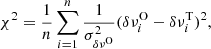
Equation (4) indicates that the sensitivity of the pulsation modes to the internal rotation can be analyzed from the behavior of the rotational kernels for each mode. In Fig. 1 we show the normalized rotational kernels computed from our adopted asteroseismological model for GD 278 for the shortest period with ℓ = 1, k = 25 (left panel) and the longest period with ℓ = 2, k = 100 (right panel). It is clear from the figure that the rotational kernels of these modes have the largest amplitudes in the region 0.5 ≲ r/R* ≲ 0.8 and in the outer part of the models, but they also have appreciable amplitudes throughout the entire stellar model. This suggests that the g modes observed in GD 278 are sensitive to the whole rotation profile, similarly to the behavior of the rotational kernels in GW Vir stars and at variance with the case of ZZ Ceti and V777 Her stars, where g modes only probe the outer parts of the star (Kawaler et al. 1999; Córsico et al. 2011; Giammichele et al. 2016).
 |
Fig. 1. Normalized rotational kernels, Kkℓ(r), for ℓ = 1, k = 25 (left panel) and ℓ = 2, k = 100 (right panel). Also indicated are the chemical profiles of H (dashed green lines) and He (dashed light blue lines). |
4. Analysis and results
4.1. Rotational splitting fits
To start this analysis, we compared the observed frequency splittings, δνO, to the theoretical frequency splittings, δνT, which were calculated by varying the rotation profile and employing the asteroseismological model presented in the previous section. This comparison was done by estimating the goodness of the match between these quantities as (Charpinet et al. 2009; Córsico et al. 2011)
 (6)
(6)
where the index i identifies each splitting and n is the number of rotational splittings considered. In this expression, each term is weighted with the inverse of the squared uncertainty of the observed frequency splittings ( ), calculated from Table 1 (Lopez et al. 2021).
4.1.1. Rigid rotation
First, we considered the simplest case for the rotation profile, which is rigid-body rotation (i.e., the angular velocity is constant throughout the star). We considered values of Ω/2π from 1 × 10⁻⁷ Hz to 1 × 10⁻⁴ Hz (corresponding to periods of ∼115 d and 3 h, respectively), and for each value we assessed the theoretical frequency splittings according to Eq. (2), where the coefficients Ckℓ are determined for each mode using Eq. (3). Considering all the observed frequency splittings associated with ℓ = 1, 2 from Table 1, we searched for the best match between the observed and the theoretical frequency splittings by calculating the χ2 (Eq. (6)). We obtained the results shown in Fig. 2, where we plot the logarithm of the quality function, χ2, in terms of Ω. In the figure, the minimum (that is, the best fit) indicates a well-defined solution for Ω ∼ 1.6 × 10⁻⁴ rad s−1, corresponding to a rotation period of ∼10.9 h. This value of the rotation period of GD 278 is in line with the determination of the rotation periods for other WDs and pre-WDs (Kawaler 2015; Córsico et al. 2019).
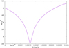 |
Fig. 2. Logarithm of the quality function, χ2, in terms of Ω, assuming rigid-body rotation. For this calculation, we have considered all the multiplets associated with ℓ = 1, 2 from Table 1. |
4.1.2. Differential rotation: The linear case
Here we lift the solid-body rotation condition and, given the exploratory nature of this work, allow for a simple case of linear differential rotation:
 (7)
(7)
where ΩC and ΩS indicate the rotation velocities at the center and at the surface, respectively. This set of linear profiles comprises both cases of increasing and decreasing Ω(r) with r and the rigid-body rotation case (ΩC = ΩS), presented in the previous section.
For the calculation of the quality function, via Eq. (6), this time we computed the theoretical frequency splittings using Eq. (4), with the rotational kernels determined by Eq. (5). We first considered all the observed frequency splittings associated with ℓ = 1, 2 from Table 1. We show the results in Fig. 3, where we plot the inverse of the quality function, 1/χ2, in the ΩS − ΩC plane, along with the loci of the solutions considering rigid rotation. By plotting the inverse of the quality function, the higher its value, the better the match between the observed and theoretical frequency splittings. It is clear from the figure that there is a range of possible solutions, that is, any solution lying on the yellow zone would have almost the same quality, therefore suggesting that the rotation could be rigid as well as differential. We indicate in the figure the best-fitting solution: (ΩS, ΩC)∼(2.1 × 10⁻⁴, 1.0 × 10⁻⁴) rad s−1. This solution, which lies close to the rigid rotation line, formally corresponds to differential rotation. This suggests that the stellar surface may be rotating slightly faster than the stellar center.
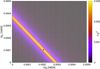 |
Fig. 3. Contour map of the inverse of the quality function, 1/χ2, showing the goodness of the fits in the plane ΩS − ΩC, considering all the observed rotational splittings associated with ℓ = 1, 2. We assume GD 278 rotates following a linear profile. The dashed green line indicates the corresponding solutions according to rigid rotation. The best-fitting solution is indicated with a black dot. |
It is interesting to study the sensitivity of our results to each of the observed frequency splittings, for which we carried out a simple procedure: we alternately removed each individual multiplet and evaluated the corresponding solution. Doing so, we find that, in general, the results remain comparable to one another, that is, (ΩS, ΩC)∼(2.0 × 10⁻⁴, 1.0 × 10⁻⁴) rad s−1 on average. However, for three cases, the results change considerably. For instance, when we excluded the multiplet associated with k = 100 from the data set, we find that ΩS becomes significantly smaller (∼6 × 10⁻⁷ rad s−1). This implies an extremely long rotation period, which would suggest that it is crucial to include this multiplet in the calculations. Its inclusion may also be justified by the fact that the frequency of the central component of this multiplet has the largest amplitude in the TESS periodogram (see Table 1 from Lopez et al. 2021). A similar situation occurs when we exclude the multiplets associated with k = 94 and 52 from the analysis.
It is worth mentioning that we also tried other types of rotation profiles, for instance two-zone profiles as presented by Charpinet et al. (2009) for PG 1159−035 and piecewise functions with three parts. The former does not allow us to make any meaningful conclusions regarding the rotation properties for GD 278, indicating that this type of profile may not be adequate for modeling the rotation in GD 278, while the latter leads to almost the same results as with the linear simple profiles of Eq. (7).
4.2. Rotation profile resulting from the evolution
Here we follow a different approach by employing a profile for the angular velocity, Ω(r), that results from detailed evolution calculations2 instead of assuming an artificial, simple profile, as in the previous sections. By using the calculated Ω(r) profile, we estimated the corresponding values of the theoretical frequency splittings.
For this procedure, we adopted a low-mass He-core model generated with MESA (see Sect. 2), characterized by M⋆ = 0.186 M⊙, Teff = 9335 K, and log(g) = 6.618 [CGS], that closely matches our asteroseismological model (that is, they have similar values of M⋆, Teff, and log(g), along with other parameters, such as the stellar radius, the H-envelope content, etc.). The rotation profile of this model is shown in Fig. 4 (solid magenta line) and is characterized by (ΩS, ΩC)∼(2.1 × 10⁻⁴, 1.5 × 10⁻⁴) rad s−1. For illustrative purposes, we also include the rigid rotation profile obtained in Sect. 4.1.1 (dashed green line) and the linear rotation profile of the best-fit model obtained in Sect. 4.1.2 (dotted black line). The MESA rotation profile and its features – which show that the rotation is barely differential and close to uniform, with the surface rotating slightly faster than the center – are the result of the CNO flashes that the progenitor of this WD experienced before entering its final cooling track, as Istrate et al. (2016b) show (see their Sect. 4.1.1.).
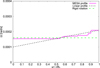 |
Fig. 4. Rotation profile of the MESA model with M⋆ = 0.186 M⊙, Teff = 9335 K, and log(g) = 6.618 [CGS] (solid magenta line), resulting from our evolutionary calculations. Also included are the rigid (dashed green line) and linear (dotted black line) rotation profiles (see text for details). |
Employing the Ω(r) profile of this model to calculate the theoretical frequency splittings corresponding to the modes of interest, using Eq. (4), we obtain the results shown in Table 3. These results indicate that, in general, there are discrepancies between the observed and the theoretical frequency splittings, but the relative differences remain below ∼15%.
Observed and theoretical frequency splittings as predicted by the rotation profile determined from evolutionary calculations.
4.3. Comparison of the results
In order to compare the main results from the previous sections, we show in Fig. 5 the observed frequency splittings (orange triangles) and the theoretical frequency splittings that result from the use of the best-fitting linear differential profile (black dots) in the case where all the observed splittings were fitted, for which we employed an asteroseismological model representative of GD 278 (generated with the LPCODE and LP-PUL codes). In addition, we show the theoretical frequency splittings as predicted from the use of the rotation profile computed with the MESA evolutionary code (magenta crosses; Table 3). All these quantities are shown in terms of the corresponding theoretical periods. The figure shows that the theoretical frequency splittings obtained via the simple linear profile and the observed frequency splittings lie close together (their differences are between ∼0.02 and 2.4 μHz), while the theoretical frequency splittings obtained from the MESA rotation profile lie slightly farther than those observed (differences between ∼0.6 and 3.6 μHz). Considering the uncertainties involved in the observed splittings and in the theoretical calculations employed in this work, we believe that these differences are not significant. Thus, we consider that there is a good agreement between the different sets of frequency splittings.
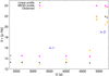 |
Fig. 5. Observed frequency splittings (orange triangles), theoretical frequency splittings obtained from the best-fitting linear differential rotation profile (black dots), and theoretical frequency splittings resulting from the rotation profile of the MESA model (magenta crosses), in terms of the corresponding theoretical periods. |
Additionally, in Fig. 6 we show the derived values of ΩS and ΩC for the solution corresponding to the best fit in the case of the linear differential rotation profiles and for the rotation profile obtained via detailed evolutionary computations with MESA. The agreement between the two approaches is clear, particularly in the value of ΩS.
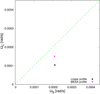 |
Fig. 6. Comparison between the values of ΩS and ΩC obtained from the best-fit solution to the linear differential rotation profiles (black dot) when considering all the splittings with ℓ = 1, 2 and the corresponding values when the rotation profile is that of the MESA evolutionary model (magenta cross). The dashed green line indicates the solutions according to rigid rotation. |
Overall, the results from the different approaches are in line with one another and with the observed properties of GD 278. The close agreement obtained when using a simple artificial rotation profile and the rotation profile that comes from fully evolutionary calculations strengthens our results, even more so given that two independent evolution codes and very different approaches were employed. Our results suggest that the rotation profile is slightly differential, but, given the uncertainties involved in these procedures (for instance, uncertainties in the frequency splittings, mode identification, and within the evolutionary approach, mainly in the rotational mixing processes), it is certainly compatible with rigid rotation, as is generally the case for WDs and pre-WDs (Córsico et al. 2019).
5. Summary and conclusions
In this work we have presented the first exploration of the internal rotation of GD 278, the (for now) only known pulsating ELM WD star that exhibits rotational frequency splittings in its periodogram, based on the mode identification presented in Lopez et al. (2021). For this purpose, we employed the observed rotational frequency splittings previously identified by Lopez et al. (2021) and compared them to theoretical splittings via rotational splitting fits. The theoretical frequency splittings were obtained by considering different ad hoc choices of the rotation profiles and employing a stellar model representative of the observed pulsation modes, which is also characterized by stellar properties within the constraints given by the spectroscopic determinations of GD 278 (Brown et al. 2020). This asteroseismological model was obtained by using the LPCODE and LP-PUL stellar evolution and pulsation codes, respectively. We also followed another approach in which we employed a rotation profile resulting from detailed evolutionary calculations obtained with the MESA evolution code and used it to infer the expected frequency splittings.
In order to carry out the rotational splitting fits, we first assumed a rigid-body rotation profile and varied the value of the (constant) angular velocity within a large range of possible values. We find that the best fit to all the observed frequency splittings corresponds to an angular velocity of ∼1.6 × 10⁻⁴ rad s−1. Next, we lifted the rigid-body rotation condition and considered a large set of linear differential rotation profiles, for different values of Ω at the surface and the center. Again, we took all the observed splittings for the fits into account, and we find that there are multiple possible solutions, the rigid-body rotation being one of them. The best-fit solution in this case corresponds to (ΩS, ΩC)∼(2.1 × 10⁻⁴, 1.0 × 10⁻⁴) rad s−1. When we analyzed the rotation profile resulting from the detailed evolutionary calculations with MESA, we found that it is characterized by (ΩS, ΩC)∼(2.1 × 10⁻⁴, 1.5 × 10⁻⁴) rad s−1. Comparing these values with the corresponding ones for the best-fitting linear rotation profile, the close agreement is evident, particularly at the surface. These values are only marginally differential and are actually compatible with rigid-body rotation. Moreover, a comparison between the observed and the theoretical frequency splittings predicted by the two profiles also shows close agreement, the theoretical splittings for the ad hoc linear case being more similar to the observed splittings.
Rotation in ELMVs and pre-ELMVs is relevant since it constitutes a very feasible mechanism candidate to explain the excitation of the pulsations observed in pre-ELM WD stars (Córsico & Althaus 2016; Istrate et al. 2016b), as well as the presence of heavy metals on the surface of ELM WDs (Gianninas et al. 2014; Hermes et al. 2014). The finding of the first pulsating ELM WD with measurable rotational frequency splittings by Lopez et al. (2021) provides, for the first time, the possibility of sounding the internal rotation in this type of star. In this sense, the present work represents only a first step in the exploration of the internal rotation in ELMVs, since there are still many uncertainties. Indeed, even with state-of-the-art evolution codes and the many advances in the observational field that help such codes improve, there is still much work to be done, for instance in the study of the angular momentum and chemical element transport mechanisms (Salaris & Cassisi 2017). The eventual detection of more ELMV stars with measurable rotational splittings can help place constraints on the physical processes involved in the development of the rotation profiles of these stars, thus making it possible to improve the current stellar models, as in other pulsating stars (Aerts 2021; Kurtz 2022). For example, few empirical constraints exist on the role of tides in the redistribution of angular momentum at these orbital periods for ELM WDs (Fuller & Lai 2012, 2014; Preece et al. 2018); studies of pulsating hot subdwarfs in close binaries show we have an incomplete understanding of all relevant physics (Preece et al. 2019). The future is promising in this regard, given the significant advances that asteroseismology has already benefited from, particularly due to the improvement in the photometry efforts coming from space missions such as Kepler/K2 (Borucki et al. 2010; Howell et al. 2014) and, more recently, the TESS and CHaracterising ExOPlanets Satellite (CHEOPS; Moya et al. 2018) programs. We expect that future missions such as the PLAnetary Transits and Oscillations (PLATO; Piotto 2018), along with the ongoing TESS and CHEOPS missions, will identify additional pulsating ELM WDs with detectable rotational splittings and more pulsation measurements.
We note that this is a different asteroseismological model than that adopted in Lopez et al. (2021). In that work, we allowed for different H envelopes in our asteroseismological fits. However, given the exploratory nature of this work, we decided to use a model that harbors a canonical (thick) envelope, for the sake of simplicity.
We are aware of the uncertainties involved in the rotational mixing processes (such as the effects of the Eddington-Sweet circulation) and in the transport of angular momentum, which translate into uncertainties in the rotation profile. However, given the exploratory nature of this work, we believe that a physical rotation profile calculated with MESA, such as the one used here, is worth considering. A detailed discussion of the uncertainties involved in the treatment of rotation in MESA is beyond the scope of the present paper.
Acknowledgments
We wish to thank our anonymous referee for the comments and suggestions that improved the original version of the paper. Support for this work was in part provided by NASA TESS Cycle 2 Grant 80NSSC20K0592 and Cycle 4 grant 80NSSC22K0737. Part of this work was supported by AGENCIA through the Programa de Modernización Tecnológica BID 1728/OC-AR, and by the PIP 112-200801-00940 grant from CONICET. This research has made use of NASA’s Astrophysics Data System.
References
- Aerts, C. 2021, Rev. Mod. Phys., 93, 015001 [Google Scholar]
- Althaus, L. G., Serenelli, A. M., & Benvenuto, O. G. 2001, MNRAS, 323, 471 [Google Scholar]
- Althaus, L. G., Serenelli, A. M., Panei, J. A., et al. 2005, A&A, 435, 631 [NASA ADS] [CrossRef] [EDP Sciences] [Google Scholar]
- Althaus, L. G., Panei, J. A., Romero, A. D., et al. 2009, A&A, 502, 207 [EDP Sciences] [Google Scholar]
- Althaus, L. G., Córsico, A. H., Isern, J., & García-Berro, E. 2010, A&ARv, 18, 471 [NASA ADS] [CrossRef] [Google Scholar]
- Althaus, L. G., Miller Bertolami, M. M., & Córsico, A. H. 2013, A&A, 557, A19 [NASA ADS] [CrossRef] [EDP Sciences] [Google Scholar]
- Althaus, L. G., Camisassa, M. E., Miller Bertolami, M. M., Córsico, A. H., & García-Berro, E. 2015, A&A, 576, A9 [NASA ADS] [CrossRef] [EDP Sciences] [Google Scholar]
- Bailer-Jones, C. A. L., Rybizki, J., Fouesneau, M., Demleitner, M., & Andrae, R. 2021, AJ, 161, 147 [Google Scholar]
- Bell, K. J., Pelisoli, I., Kepler, S. O., et al. 2018, A&A, 617, A6 [NASA ADS] [CrossRef] [EDP Sciences] [Google Scholar]
- Bell, K. J., Córsico, A. H., Bischoff-Kim, A., et al. 2019, A&A, 632, A42 [NASA ADS] [CrossRef] [EDP Sciences] [Google Scholar]
- Bognár, Z., Paparó, M., Córsico, A. H., Kepler, S. O., & Győrffy, Á. 2014, A&A, 570, A116 [NASA ADS] [CrossRef] [EDP Sciences] [Google Scholar]
- Borucki, W. J., Koch, D., Basri, G., et al. 2010, Science, 327, 977 [Google Scholar]
- Bradley, P. A. 2001, ApJ, 552, 326 [NASA ADS] [CrossRef] [Google Scholar]
- Brickhill, A. J. 1975, MNRAS, 170, 405 [NASA ADS] [CrossRef] [Google Scholar]
- Brown, W. R., Kilic, M., Allende Prieto, C., & Kenyon, S. J. 2010, ApJ, 723, 1072 [Google Scholar]
- Brown, W. R., Gianninas, A., Kilic, M., Kenyon, S. J., & Allende Prieto, C. 2016, ApJ, 818, 155 [Google Scholar]
- Brown, W. R., Kilic, M., Kosakowski, A., et al. 2020, ApJ, 889, 49 [Google Scholar]
- Brown, W. R., Kilic, M., Kosakowski, A., & Gianninas, A. 2022, ApJ, 933, 94 [NASA ADS] [CrossRef] [Google Scholar]
- Burgers, J. M. 1969, Flow Equations for Composite Gases (New York: Academic Press) [Google Scholar]
- Calcaferro, L. M., Córsico, A. H., & Althaus, L. G. 2016, A&A, 589, A40 [NASA ADS] [CrossRef] [EDP Sciences] [Google Scholar]
- Calcaferro, L. M., Córsico, A. H., & Althaus, L. G. 2017, A&A, 607, A33 [NASA ADS] [CrossRef] [EDP Sciences] [Google Scholar]
- Calcaferro, L. M., Althaus, L. G., & Córsico, A. H. 2018a, A&A, 614, A49 [NASA ADS] [CrossRef] [EDP Sciences] [Google Scholar]
- Calcaferro, L. M., Córsico, A. H., Althaus, L. G., Romero, A. D., & Kepler, S. O. 2018b, A&A, 620, A196 [EDP Sciences] [Google Scholar]
- Cantiello, M., Mankovich, C., Bildsten, L., Christensen-Dalsgaard, J., & Paxton, B. 2014, ApJ, 788, 93 [Google Scholar]
- Charpinet, S., Fontaine, G., & Brassard, P. 2009, Nature, 461, 501 [NASA ADS] [CrossRef] [Google Scholar]
- Córsico, A. H., & Althaus, L. G. 2006, A&A, 454, 863 [NASA ADS] [CrossRef] [EDP Sciences] [Google Scholar]
- Córsico, A. H., & Althaus, L. G. 2016, A&A, 585, A1 [NASA ADS] [CrossRef] [EDP Sciences] [Google Scholar]
- Córsico, A. H., Althaus, L. G., Miller Bertolami, M. M., & Werner, K. 2007a, A&A, 461, 1095 [NASA ADS] [CrossRef] [EDP Sciences] [Google Scholar]
- Córsico, A. H., Miller Bertolami, M. M., Althaus, L. G., Vauclair, G., & Werner, K. 2007b, A&A, 475, 619 [NASA ADS] [CrossRef] [EDP Sciences] [Google Scholar]
- Córsico, A. H., Althaus, L. G., Kepler, S. O., Costa, J. E. S., & Miller Bertolami, M. M. 2008, A&A, 478, 869 [NASA ADS] [CrossRef] [EDP Sciences] [Google Scholar]
- Córsico, A. H., Althaus, L. G., Miller Bertolami, M. M., & García-Berro, E. 2009a, A&A, 499, 257 [NASA ADS] [CrossRef] [EDP Sciences] [Google Scholar]
- Córsico, A. H., Althaus, L. G., Miller Bertolami, M. M., González Pérez, J. M., & Kepler, S. O. 2009b, ApJ, 701, 1008 [Google Scholar]
- Córsico, A. H., Althaus, L. G., Kawaler, S. D., et al. 2011, MNRAS, 418, 2519 [CrossRef] [Google Scholar]
- Córsico, A. H., Althaus, L. G., Miller Bertolami, M. M., & Bischoff-Kim, A. 2012, A&A, 541, A42 [CrossRef] [EDP Sciences] [Google Scholar]
- Córsico, A. H., Althaus, L. G., Serenelli, A. M., et al. 2016, A&A, 588, A74 [NASA ADS] [CrossRef] [EDP Sciences] [Google Scholar]
- Córsico, A. H., Althaus, L. G., Miller Bertolami, M. M., & Kepler, S. O. 2019, A&ARv, 27, 7 [Google Scholar]
- Córsico, A. H., Uzundag, M., Kepler, S. O., et al. 2021, A&A, 645, A117 [EDP Sciences] [Google Scholar]
- Córsico, A. H., Uzundag, M., Kepler, S. O., et al. 2022, A&A, 659, A30 [NASA ADS] [CrossRef] [EDP Sciences] [Google Scholar]
- Cowling, T. G., & Newing, R. A. 1949, ApJ, 109, 149 [NASA ADS] [CrossRef] [Google Scholar]
- Deheuvels, S., García, R. A., Chaplin, W. J., et al. 2012, ApJ, 756, 19 [Google Scholar]
- Fontaine, G., & Brassard, P. 2008, PASP, 120, 1043 [NASA ADS] [CrossRef] [Google Scholar]
- Fuller, J., & Lai, D. 2012, MNRAS, 421, 426 [NASA ADS] [Google Scholar]
- Fuller, J., & Lai, D. 2014, MNRAS, 444, 3488 [NASA ADS] [CrossRef] [Google Scholar]
- Gaia Collaboration 2020, VizieR Online Data Catalog: I/350 [Google Scholar]
- Gentile Fusillo, N. P., Tremblay, P.-E., Gänsicke, B. T., et al. 2019, MNRAS, 482, 4570 [Google Scholar]
- Giammichele, N., Fontaine, G., Brassard, P., & Charpinet, S. 2016, ApJS, 223, 10 [NASA ADS] [CrossRef] [Google Scholar]
- Giammichele, N., Charpinet, S., Brassard, P., & Fontaine, G. 2017, A&A, 598, A109 [NASA ADS] [CrossRef] [EDP Sciences] [Google Scholar]
- Gianninas, A., Hermes, J. J., Brown, W. R., et al. 2014, ApJ, 781, 104 [NASA ADS] [CrossRef] [Google Scholar]
- Gianninas, A., Kilic, M., Brown, W. R., Canton, P., & Kenyon, S. J. 2015, ApJ, 812, 167 [Google Scholar]
- Gianninas, A., Curd, B., Fontaine, G., Brown, W. R., & Kilic, M. 2016, ApJ, 822, L27 [Google Scholar]
- Heger, A., Langer, N., & Woosley, S. E. 2000, ApJ, 528, 368 [NASA ADS] [CrossRef] [Google Scholar]
- Heger, A., Woosley, S. E., & Spruit, H. C. 2005, ApJ, 626, 350 [Google Scholar]
- Hermes, J. J., Montgomery, M. H., Winget, D. E., et al. 2012, ApJ, 750, L28 [Google Scholar]
- Hermes, J. J., Montgomery, M. H., Gianninas, A., et al. 2013a, MNRAS, 436, 3573 [Google Scholar]
- Hermes, J. J., Montgomery, M. H., Winget, D. E., et al. 2013b, ApJ, 765, 102 [Google Scholar]
- Hermes, J. J., Gänsicke, B. T., Koester, D., et al. 2014, MNRAS, 444, 1674 [NASA ADS] [CrossRef] [Google Scholar]
- Hermes, J. J., Kawaler, S. D., Bischoff-Kim, A., et al. 2017, ApJ, 835, 277 [Google Scholar]
- Howell, S. B., Sobeck, C., Haas, M., et al. 2014, PASP, 126, 398 [Google Scholar]
- Istrate, A. G., Fontaine, G., Gianninas, A., et al. 2016a, A&A, 595, L12 [NASA ADS] [CrossRef] [EDP Sciences] [Google Scholar]
- Istrate, A. G., Marchant, P., Tauris, T. M., et al. 2016b, A&A, 595, A35 [NASA ADS] [CrossRef] [EDP Sciences] [Google Scholar]
- Itoh, N., Kohyama, Y., & Takeuchi, H. 1987, ApJ, 317, 733 [NASA ADS] [CrossRef] [Google Scholar]
- Jeffery, C. S., & Saio, H. 2013, MNRAS, 435, 885 [Google Scholar]
- Kawaler, S. D. 2015, ASP Conf. Ser., 493, 65 [NASA ADS] [Google Scholar]
- Kawaler, S. D., Sekii, T., & Gough, D. 1999, ApJ, 516, 349 [NASA ADS] [CrossRef] [Google Scholar]
- Kilic, M., Brown, W. R., Allende Prieto, C., et al. 2011, ApJ, 727, 3 [Google Scholar]
- Kilic, M., Hermes, J. J., Córsico, A. H., et al. 2018, MNRAS, 479, 1267 [Google Scholar]
- Koester, D., Voss, B., Napiwotzki, R., et al. 2009, A&A, 505, 441 [NASA ADS] [CrossRef] [EDP Sciences] [Google Scholar]
- Kosakowski, A., Kilic, M., Brown, W. R., & Gianninas, A. 2020, ApJ, 894, 53 [Google Scholar]
- Kurtz, D. W. 2022, ARA&A, 60, 31 [NASA ADS] [CrossRef] [Google Scholar]
- Kurtz, D. W., Saio, H., Takata, M., et al. 2014, MNRAS, 444, 102 [Google Scholar]
- Ledoux, P. 1951, ApJ, 114, 373 [Google Scholar]
- Li, Z., Chen, X., Chen, H.-L., & Han, Z. 2019, ApJ, 871, 148 [NASA ADS] [CrossRef] [Google Scholar]
- Lopez, I. D., Hermes, J. J., Calcaferro, L. M., et al. 2021, ApJ, 922, 220 [NASA ADS] [CrossRef] [Google Scholar]
- Maxted, P. F. L., Serenelli, A. M., Miglio, A., et al. 2013, Nature, 498, 463 [Google Scholar]
- Maxted, P. F. L., Serenelli, A. M., Marsh, T. R., et al. 2014, MNRAS, 444, 208 [Google Scholar]
- Moya, A., Barceló Forteza, S., Bonfanti, A., et al. 2018, A&A, 620, A203 [NASA ADS] [CrossRef] [EDP Sciences] [Google Scholar]
- Paxton, B., Bildsten, L., Dotter, A., et al. 2011, ApJS, 192, 3 [Google Scholar]
- Paxton, B., Cantiello, M., Arras, P., et al. 2013, ApJS, 208, 4 [Google Scholar]
- Paxton, B., Marchant, P., Schwab, J., et al. 2015, ApJS, 220, 15 [Google Scholar]
- Paxton, B., Schwab, J., Bauer, E. B., et al. 2018, ApJS, 234, 34 [NASA ADS] [CrossRef] [Google Scholar]
- Paxton, B., Smolec, R., Schwab, J., et al. 2019, ApJS, 243, 10 [Google Scholar]
- Pelisoli, I., Kepler, S. O., Koester, D., et al. 2018, MNRAS, 478, 867 [Google Scholar]
- Piotto, G. 2018, European Planetary Science Congress, EPSC2018-969 [Google Scholar]
- Preece, H. P., Tout, C. A., & Jeffery, C. S. 2018, MNRAS, 481, 715 [NASA ADS] [CrossRef] [Google Scholar]
- Preece, H. P., Tout, C. A., & Jeffery, C. S. 2019, MNRAS, 485, 2889 [NASA ADS] [CrossRef] [Google Scholar]
- Ricker, G. R., Winn, J. N., Vanderspek, R., et al. 2015, J. Astron. Telesc. Instrum. Syst., 1, 014003P [Google Scholar]
- Ritter, H. 1988, A&A, 202, 93 [NASA ADS] [Google Scholar]
- Romero, A. D., Córsico, A. H., Althaus, L. G., et al. 2012, MNRAS, 420, 1462 [Google Scholar]
- Salaris, M., & Cassisi, S. 2017, R. Soc. Open Sci., 4, 170192P [NASA ADS] [CrossRef] [Google Scholar]
- Spruit, H. C. 2002, A&A, 381, 923 [CrossRef] [EDP Sciences] [Google Scholar]
- Sun, M., & Arras, P. 2018, ApJ, 858, 14 [NASA ADS] [CrossRef] [Google Scholar]
- Unno, W., Osaki, Y., Ando, H., Saio, H., & Shibahashi, H. 1989, Nonradial Oscillations of Stars (Tokyo: University of Tokyo Press) [Google Scholar]
- Uzundag, M., Córsico, A. H., Kepler, S. O., et al. 2022, MNRAS, 513, 2285 [NASA ADS] [CrossRef] [Google Scholar]
- Van Grootel, V., Fontaine, G., Brassard, P., & Dupret, M.-A. 2013, ApJ, 762, 57 [Google Scholar]
- Wang, K., Zhang, X., & Dai, M. 2020, ApJ, 888, 49 [Google Scholar]
- Winget, D. E., & Kepler, S. O. 2008, ARA&A, 46, 157 [Google Scholar]
All Tables
Mode identifications and observed frequency splittings for GD 278 (adapted from Lopez et al. 2021).
Comparison between the observed periods of GD 278 and the theoretical periods of the adopted asteroseismological model characterized by M⋆ = 0.186 M⊙, Teff = 9335 K, and log(g) = 6.618 [CGS].
Observed and theoretical frequency splittings as predicted by the rotation profile determined from evolutionary calculations.
All Figures
|
Fig. 1. Normalized rotational kernels, Kkℓ(r), for ℓ = 1, k = 25 (left panel) and ℓ = 2, k = 100 (right panel). Also indicated are the chemical profiles of H (dashed green lines) and He (dashed light blue lines). |
| In the text | |
|
Fig. 2. Logarithm of the quality function, χ2, in terms of Ω, assuming rigid-body rotation. For this calculation, we have considered all the multiplets associated with ℓ = 1, 2 from Table 1. |
| In the text | |
|
Fig. 3. Contour map of the inverse of the quality function, 1/χ2, showing the goodness of the fits in the plane ΩS − ΩC, considering all the observed rotational splittings associated with ℓ = 1, 2. We assume GD 278 rotates following a linear profile. The dashed green line indicates the corresponding solutions according to rigid rotation. The best-fitting solution is indicated with a black dot. |
| In the text | |
|
Fig. 4. Rotation profile of the MESA model with M⋆ = 0.186 M⊙, Teff = 9335 K, and log(g) = 6.618 [CGS] (solid magenta line), resulting from our evolutionary calculations. Also included are the rigid (dashed green line) and linear (dotted black line) rotation profiles (see text for details). |
| In the text | |
|
Fig. 5. Observed frequency splittings (orange triangles), theoretical frequency splittings obtained from the best-fitting linear differential rotation profile (black dots), and theoretical frequency splittings resulting from the rotation profile of the MESA model (magenta crosses), in terms of the corresponding theoretical periods. |
| In the text | |
|
Fig. 6. Comparison between the values of ΩS and ΩC obtained from the best-fit solution to the linear differential rotation profiles (black dot) when considering all the splittings with ℓ = 1, 2 and the corresponding values when the rotation profile is that of the MESA evolutionary model (magenta cross). The dashed green line indicates the solutions according to rigid rotation. |
| In the text | |
Current usage metrics show cumulative count of Article Views (full-text article views including HTML views, PDF and ePub downloads, according to the available data) and Abstracts Views on Vision4Press platform.
Data correspond to usage on the plateform after 2015. The current usage metrics is available 48-96 hours after online publication and is updated daily on week days.
Initial download of the metrics may take a while.