| Issue |
A&A
Volume 636, April 2020
|
|
|---|---|---|
| Article Number | A120 | |
| Number of page(s) | 11 | |
| Section | Stellar atmospheres | |
| DOI | https://doi.org/10.1051/0004-6361/202037890 | |
| Published online | 29 April 2020 | |
The 3D non-LTE solar nitrogen abundance from atomic lines
1
Theoretical Astrophysics, Department of Physics and Astronomy, Uppsala University,
Box 516,
751 20
Uppsala,
Sweden
e-mail: This email address is being protected from spambots. You need JavaScript enabled to view it.
2
Centre Spatial de Liège, Université de Liége,
avenue Pré Aily,
4031
Angleur-Liège,
Belgium
3
Space sciences, Technologies and Astrophysics Research (STAR) Institute, Université de Liège,
Allée du 6 août, 17 B5C,
4000
Liège, Belgium
4
Research School of Astronomy and Astrophysics, Australian National University,
Canberra,
ACT 2600, Australia
5
Stellar Astrophysics Centre, Department of Physics and Astronomy, Aarhus University,
Ny Munkegade 120,
8000
Aarhus C,
Denmark
Received:
5
March
2020
Accepted:
27
March
2020
Abstract
Nitrogen is an important element in various fields of stellar and Galactic astronomy, and the solar nitrogen abundance is crucial as a yardstick for comparing different objects in the cosmos. In order to obtain a precise and accurate value for this abundance, we carried out N I line formation calculations in a 3D radiative-hydrodynamic STAGGER model solar atmosphere in full 3D non-local thermodynamic equilibrium (non-LTE). We used a model atom that includes physically motivated descriptions for the inelastic collisions of N I with free electrons and with neutral hydrogen. We selected five N I lines of high excitation energy to study in detail, based on their strengths and on their being relatively free of blends. We found that these lines are slightly strengthened from non-LTE photon losses and from 3D granulation effects, resulting in negative abundance corrections of around − 0.01 dex and − 0.04 dex, respectively. Our advocated solar nitrogen abundance is log ɛN = 7.77, with the systematic 1σ uncertainty estimated to be 0.05 dex. This result is consistent with earlier studies after correcting for differences in line selections and equivalent widths.
Key words: atomic processes / radiative transfer / line: formation / Sun: abundances / Sun: photosphere / stars: abundances
© ESO 2020
1 Introduction
Nitrogen is an important element in many different areas of astrophysics. Its dominant isotope, 14N, is synthesised via the CNO-cycle: its main origins in the universe are thought to be asymptotic giant branch stars and, at least at low metallicities, fast-rotating massive stars (e.g. Karakas & Lattanzio 2014; Vincenzo et al. 2016). Nitrogen abundances shed light on the structure and evolution of stars, and of galaxies, via measurement in a variety of different cosmic objects including measured in hot and cool stars in our Galaxy and its satellites (e.g. Schiavon et al. 2017; Magrini et al. 2018; Lyubimkov et al. 2019; Salgado et al. 2019), in interstellar media (e.g. Belfiore et al. 2017; Esteban & García-Rojas 2018), and in damped Lyman-α systems (e.g. Zafar et al. 2014; Berg et al. 2019).
The solar abundance of nitrogen is then crucial for having a solid yardstick with which to compare the different cosmic objects discussed above. Nitrogen forms highly volatile compounds that do not efficiently condense into grains; thus its abundance as measured from meteorites does not reflect the initial abundance of the solar system at the time of its birth (Lodders 2019). As such, the most reliable way to infer the initial solar system abundance of nitrogen is through spectroscopy of the solar photosphere.
The challenge is to derive the solar abundance with both high precision and high accuracy. In the current standard set of solar abundances (Asplund et al. 2009), nitrogen has log ɛN = 7.83 ± 0.051. This value is primarily based on optical and near-infrared N I lines (log ɛN = 7.78 ± 0.04), and near-infrared rotational-vibrational (Δν = 1) NH lines (log ɛN = 7.88 ± 0.03); secondary diagnostics include the near-infrared pure-rotational (Δν = 0) NH lines as well as various CN electronic bands. For their analysis, the authors employed a three dimensional (3D) radiative-hydrodynamic model of the solar atmosphere, calculated using the STAGGER code (Nordlund & Galsgaard 1995; Collet et al. 2018); this particular model was discussed in, for example, Sect. 3 of Scott et al. (2015).
There have been surprisingly few other recent studies of the solar nitrogen abundance presented in the literature, at least after considering the broad importance of this element in astronomy. Caffau et al. (2009) presented an analysis of the N I lines using an independent 3D model, calculated using CO5BOLD (Freytag et al. 2012). Their advocated value is log ɛN = 7.86 ± 0.12, which is 0.08 dex higher than the N I value from Asplund et al. (2009), but nevertheless consistent within the stipulated 1σ uncertainties.
A potential shortcoming of these two previous studies lies in their treatment of departures from local thermodynamic equilibrium (LTE). There is a general consensus that N I is susceptible to departures from LTE, that may amount to around 0.05 dex in solar type stars (Takeda & Honda 2005). Asplund et al. (2009) applied non-LTE abundance corrections from Rentzsch-Holm (1996) based on a one-dimensional (1D) model solar, while Caffau et al. (2009) calculated non-LTE abundance corrections on their temporally- and horizontally-averaged 3D model.
There are two important developments that make revisiting the nitrogen abundance inferred from N I lines of importance. First, it is now possible to carry out full 3D non-LTE radiative transfer for spectrum synthesis and abundance analyses without making significant compromises on the resolution of the adopted model solar atmosphere,nor on the complexity of the non-LTE model atom. In this approach, the departures from LTE are calculated consistently with the 3D model solar atmosphere itself, taking into full consideration non-vertical radiative transfer.
Secondly, non-LTE model atoms can now be constructed that are much more reliable than ever before. This is in large part thanks to the rapid progress made recently in modelling low-energy inelastic collisions, with both free electrons, and neutral hydrogen. Apoor description of such processes can often be the main limitation in non-LTE models (Barklem 2016a). In the past, classical or semi-empirical approaches were commonly used to model them, such as that of van Regemorter (1962) for electron collisions, and the Drawin recipe (Drawin 1969, 1968) as presented in Steenbock & Holweger (1984) and Lambert (1993) for hydrogen collisions. These are of limited validity however; the latter being so uncertain, a fudge factor SH is usually applied and calibrated so as to match the observations. For nitrogen, the situation today is more positive: ab initio cross-sections for the electron collisions are available via the B-spline R-matrix (BSR) method (Wang et al. 2014); cross-sections for the hydrogen collisions involving low-lying levels have been calculated via the Landau-Zener model coupled with a linear combination of atomic orbitals (LCAO) method (Amarsi & Barklem 2019), and for more highly-excited levels they can be estimated using the free electron method (Kaulakys 1985, 1986, 1991), which is valid in the Rydberg regime.
Our aim here is to revisit the solar nitrogen abundance using the latest spectrum synthesis methods. Similar to our recent studies of oxygen (Amarsi et al. 2018a) and carbon (Amarsi et al. 2019), we use the 3D non-LTE radiative transfer code BALDER (our modified version of MULTI3D), a 3D STAGGER model solar atmosphere, and a new non-LTE model atom that is based on the BSR and LCAO/free electron methods for the inelastic collisions. We demonstrated that this approach successfully reproduce the centre-to-limb variations of the O I 777 nm lines, as well as various lines of C I, without having to resort to any calibrated fudge factors that would always be necessary with the Drawin recipe and with 1D models.
The rest of this paper is structured as follows. We review the method in Sect. 2. We discuss the nature of the 3D non-LTE effects on N I in Sect. 3. We present and discuss our advocated solar nitrogen abundance in Sect. 4, and compare the result with those from previous studies. We present a summary and some concluding remarks in Sect. 5.
2 Method
2.1 Abundance indicators and observational data
There are more than 20 different N Ilines in the solar spectrum that have been used as abundance indicators in the past (Grevesse et al. 1990; Biémont et al. 1990; Caffau et al. 2009). The lines are all of rather high excitation energy (χlow ≳ 10.3 eV), forming deep in the solar atmosphere as we show in Fig. 1 (− 0.2 ≲ log τR ≲ 0.7, at solar disk centre). All tend to be very weak and suffering from blends or from perturbations from nearby lines. After carefully considering their shapes in the solar atlas, we selected just five N I lines that are strong enough and sufficiently clean to serve as reliable abundance indicators.
We list the parameters of the five abundance indicators in Table 1. Their oscillator strengths were drawn from Tachiev & Froese Fischer (2002), which were calculated using the multiconfigurational Hartree-Fock (MCHF) method, including relativistic effects via the Breit-Pauli Hamiltonian to represent LS-term mixing (Froese Fischer 1997; Froese Fischer et al. 2016). Their calculations were performed with an early version of the MCHF Atomic Structure Package, ATSP2K (Froese Fischer 2000; Froese Fischer et al. 2007). As a sanity check, we carried out our own fully-relativistic multiconfigurational Dirac-Hartree-Fock (MCDHF) calculations, using the latest version of the GRASP code (Froese Fischer et al. 2019), that is available as open-source2. The agreement between these two approaches was found to be better than 0.01 dex.
We present the measured equivalent widths of the N I features, the CN blends and, thus, the N I lines, in Table 2. Even with our stringent selection, four of the five selected N I lines are significantly blended by CN lines of high excitation energy. Although these CN lines were detected via a 3D LTE synthesis, the CN contribution to the equivalent widths of the N I features were estimated empirically by measuring the strengths of neighbouring CN lines in the same band. This approach is preferred over using the 3D LTE synthesis to estimate the blending contribution, because it is less sensitive to modelling errors: namely, neglected non-LTE effects and deficiencies in the 3D model atmosphere in the cool upper regions where the molecules form, log τR ≈−1.5; as well as systematic errors in the absolute log gf values of the CN lines. Since the CN blends form much higher in the atmosphere compared to the N I lines, their contribution to the total equivalent width can therefore simply be subtracted, to give the N I equivalent widths.
Although the equivalent width of the N I 822 nm line is not significantly affected by CN blends, the wings of this line are visibly perturbed in the solar spectrum. Consequently, the five N I lines are given equal weight in the abundance analysis presented below.
To minimise the impact of blends, the analysis is based on disk-centre intensities rather than on disk-integrated fluxes. The equivalent widths were measured in both the Jungfraujoch (Delbouille et al. 1973) and Kitt Peak (Neckel & Labs 1984) atlases, both data sets having extremely high signal-to-noise ratios and spectral resolutions (Delbouille & Roland 1995; Neckel 1999). The two measurements of WN i agree to better than 5%, and the final values in Table 2 are the average of the two atlases.
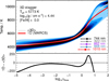 |
Fig. 1 Temperatures as functions of Rosseland mean optical depth for the different model solar atmospheres considered in this study (top), and residual difference between the 1D and ⟨3D⟩ models (bottom). The optical depths corresponding to peak line formation as well as the interquartile ranges of the 5 N I lines are indicated; these values are based on the line-integrated contribution function to the line depression in the disk-centre intensity (Eq. (15) of Amarsi 2015), calculated using the ⟨3D⟩ model solar atmosphere. |
Parameters of the five N I lines used in the abundance analysis.
Equivalent widths of the N I features, measured at solar disk centre.
2.2 Line formation calculations
The 3D non-LTE radiative transfer code BALDER, our modified version of MULTI3D (Leenaarts & Carlsson 2009), was used to calculate synthetic solar spectra to compare to the observational data. More details about the code can be found in our previous papers (e.g. Amarsi et al. 2018b). In short, BALDER solves the radiative transfer equation simultaneously with the equations of statistical equilibrium, following the single-transition preconditioning scheme described in Sect. 2.4 of Rybicki & Hummer (1992). During the non-LTE iterations, an integral solver is used to solve the radiative transfer equation on short characteristics (Ibgui et al. 2013). Once the populations have converged, a final calculation is carried out on long characteristics. The true continuum intensity is also calculated at this point, by carrying out another calculation with all line opacities set to zero. The equation-of-state (EOS) and background line and continuous opacities are calculated using the code BLUE (Sect. 2.1.2 of Amarsi et al. 2016).
The two main inputs for BALDER are the model atmosphere, and the non-LTE model atom. We discuss these in turn in Sects. 2.3 and 2.4, below. For a given model atmosphere and a given non-LTE model atom, radiative transfer calculations were performed independently for different nitrogen abundances, in steps of 0.2 dex around a central value of log ɛN = 7.83.
2.3 Model solar atmospheres
We illustrate the different model solar atmospheres used in this work in Fig. 1. The main results of this study are based on a 3D radiative-hydrodynamic simulation that was calculated using the STAGGER code (Nordlund & Galsgaard 1995; Collet et al. 2018). This model has a mean effective temperature of 5773 K and was constructed using the solar abundance set of Asplund et al. (2009); this abundance set was also adopted when calculating the EOS and background opacities for the line formation calculations. More details about this 3D model can be found in our earlier studies of 3D non-LTE line formation in the Sun (Amarsi et al. 2018a, 2019). The detailed 3D non-LTE radiative transfer was calculated on eight snapshots of this model, equally spaced over 21 hours of solar time.
In addition, calculations were performed on two different 1D hydrostatic model solar atmospheres, to allow for a differential study of the 3D effects and also to aid future comparisons of this work. First, calculations were performed on the temporally- and horizontally-average of the 3D model solar atmosphere. Details of its construction can be found in Amarsi et al. (2018a). The solar abundance set of Asplund et al. (2009) was adopted when calculating the EOS and background opacities for the line formation calculations. We refer to this as the ⟨3D⟩ model hereafter.
Secondly, calculations were performed on the standard 1D MARCS model solar atmosphere (Gustafsson et al. 2008). This model was constructed using the solar abundance set of Grevesse et al. (2007); as such, we took care to adopt this same abundance set when calculating the EOS and background opacities for the line formation calculations. We verified that the MARCS model gives consistent results (to better than 0.01 dex in terms of inferred abundances) with our ATMO model (Magic et al. 2013, Appendix A), the latter being constructed with an identical equation of state and radiative transfer solver as used for the 3D STAGGER model. This is not too surprising, given that both the MARCS and the ATMO models were constructed with the same underlying physical assumptions (1D, hydrostatic, LTE) with identical mixing-length descriptions (Böhm-Vitense 1958; Henyey et al. 1965) and very similar background opacity data sources as well as EOS. We refer to the MARCS model as the 1D model hereafter.
In general it is necessary to include two tuneable line broadening parameters in spectral line synthesis calculations based on 1D model atmospheres (e.g. Gray 2008, Chap. 17): microturbulence ξmic, and macroturbulence ξmac. These roughly account for line broadening due to velocity gradients and temperature inhomogeneities associated with stellar granulation, on scales much shorter than and much larger than one optical path length, respectively. For the 1D calculations with BALDER, a depth-independent microturbulence of ξmic = 1 km s−1 was adopted; the weak nitrogen lines are not particularly sensitive to this parameter, and increasing ξmic even to 2 km s−1 only changed the results by 0.01 dex for the strongest lines in the line selection (the N I 822 and 868 nm). Macroturbulent broadening as defined above conserves equivalent widths, as such the choice of ξmac is inconsequential to the analysis presented here. Radiative transfer calculations on 3D model atmospheres naturally take into account these broadening effects without having to include extra tuneable parameters (Asplund et al. 2000).
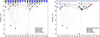 |
Fig. 2 Grotrian diagrams for N I in the comprehensive starting non-LTE model atom (left), and in the resulting non-LTE model atom after reducing its complexity (right). Energy levels are indicated as short black horizontal lines; those levels for which fine structure is not resolved are indicated as short blue horizontal lines, and super levels are shown as long blue horizontal lines. All bound–bound radiative transitions considered in the non-LTE iterations are shown in grey. The five abundance indicators are labelled and marked specially in the right panel. |
2.4 Non-LTE model atom
A new non-LTE model atom for N I was constructed for this study. The method of construction follows that presented in our previous studies of O I (Amarsi et al. 2018a) and C I (Amarsi et al. 2019); we present an overview of the different ingredients in the model here, and refer the reader to those papers for further details.
We illustrate the “full” and “standard” non-LTE model atoms in Fig. 2. As in our previous studies, the standard non-LTE model atom that was used for the production runs was generated by first constructing a full model, in which we tried to include a complete description of N I, without attempting to minimise the overall complexity of the model. The complexity of the full model was then reduced by averaging together certain levels and transitions, so as to reduce the computational cost of the 3D non-LTE calculations, while retaining the most relevant physics in the model and thus not compromising the accuracy of the final results. It is important to note that prior to carrying out the final solution of the radiative transfer equation, the departure coefficients from the standard model were applied to the LTE populations of the full model. This was done to ensure that the energy levels, oscillator strengths, partition functions, and so on were as accurate as possible for the calculation of the synthetic solar spectra.
The full model consists of 230 levels of N I along with the low-lying 2p 2 3P0,1,2 and 2p 2 1D2 levels of N I. The primary data source was the NIST Atomic Spectra Database (Kramida et al. 2015): LSJ energies and oscillator strengths were taken from here, the original data coming from Moore (1993), and from Zhu et al. (1989), Bell & Berrington (1991), Hibbert et al. (1991), Musielok et al. (1995), Tachiev & Froese Fischer (2002), and the unpublished 1994 Opacity Project data set of Burke and Lennon. Missing atomic data were then included, taking theoretical LS energies, oscillator strengths, photoionisation cross-sections, and natural broadening coefficients from The Opacity Project Database (TOPbase; Cunto et al. 1993). Broadening coefficients via elastic neutral hydrogen collisions were obtained by interpolating the tables of Anstee, Barklem, and O’Mara (ABO; Anstee & O’Mara 1995; Barklem & O’Mara 1997; Barklem et al. 1998).
The cross-sections for excitation and ionisation of N I via electron collisions:
 (1)
(1)
 (2)
(2)
were taken from Wang et al. (2014), which are based on the BSR method (Zatsarinny 2006). These data are complete up to 2p 2 3d 2D. For higher levels, for electron excitation the semi-empirical recipe of van Regemorter (1962) was used (this recipe is based on the permitted radiative transition probability; for missing permitted lines, and for forbidden lines, flat dimensionless collision strengths of ϒ = 1.0, and of ϒ = 0.1, were respectively assumed instead); while for electron ionisation, the empirical recipe of Allen (1973) was used.
The cross-sections for excitation and charge transfer of N I via hydrogen collisions:
 (3)
(3)
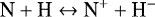 (4)
(4)
were taken from (Amarsi & Barklem 2019), which were calculated using the Landau-Zener model for non-adiabatic transition probabilities combined with a two-electron LCAO method for the electronic structure (Barklem 2016b; see also the asymptotic method of Belyaev 2013). As motivated in Amarsi et al. (2018a, 2019), we added to the LCAO cross-sections, the cross-sections calculated using the Barklem (2017) code that implements the free electron method (Kaulakys 1985, 1986, 1991), and redistributing the data to account for different spin states (see Eqs. (8) and (9) of Barklem 2016a). Finally, the cross-sections for ionisation of N I via hydrogen collisions:
 (5)
(5)
were calculated using Eq. (8) of Kaulakys (1985).
The TOPbase oscillator strengths and the collisional cross-sections adopted here were all calculated under LS-coupling; that is, without resolving fine structure. However, the non-LTE model atom does resolve fine structure. For consistency, the LS oscillator strengths and collisional cross-sections were redistributed onto the LSJ levels. The TOBbase lines connecting two LSJ levels from NIST were redistributed using the tables in Sect. 27 of Allen (1973); this is valid under the assumption of pure LS coupling.
The collisions were redistributed to account for fine structure in the same way that was described inSect. 2.4.1 of Amarsi et al. (2018a). In summary, the rate coefficient from one LS level x, to another LS level y, was redistributed among LSJ sublevels by dividing the LS rate coefficient in a given direction x → y by the total number of LSJ target sublevels (y1, y2, …). This preserves the total LS rate per perturber per unit time into the LS level y, in the limit where the energy splitting due to fine structure goes to zero. The rate coefficient in the reverse direction y →x was then calculated strictly using the principle of detailed balance. Finally, collisions within fine structure sublevels (y1 ↔ y2, …) were introduced and given arbitrarily large rates. This ensures that the total LS rate per perturber per unit time in the reverse direction (y → x) is also exactly preserved, again in the limit where the energy splitting due to fine structure goes to zero.
The standard model was constructed by reducing the full model, in the following way. First, the fine structure in all LSJ NIST levels within 1.52 eV of the ionisation limit of N I (2p2 4p 4Do and above), as well as in the ground level of N I, were collapsed to LS terms, and the transitions connecting them were also collapsed, in the manner described in Sect. 2.3.3 of Amarsi & Asplund (2017), based on the formulae given in Martin & Wiese (1999). Second, all levels within 0.88 eV of the ionisation limit of N I were grouped into two super levels, corresponding to the 2S + 1 = 2 (82 levels) and 4 (80 levels) spin systems. The super levels, and corresponding super transitions, were constructed in an analogous way to how all fine structure were collapsed.
We verified that the standard and full non-LTE model atoms give consistent results, at least on the ⟨3D⟩ model solar atmosphere. The difference between the abundances inferred from the full and standard non-LTE model atoms was less than 0.0001 dex for the five of the lines in Table 1.
3 3D non-LTE effects
3.1 Nature of the non-LTE effect
To understand the nature of the non-LTE effects, we illustrate the departure coefficients for the different N I levels inFig. 3. The overall picture is qualitatively similar to that of previous studies (compare with Fig. 1 of Caffau et al. 2009). The models indicate that N I suffers from photon losses in its lines of highexcitation energy: photons are scattered to large distances in the solar atmosphere and lost, causing a population cascade to lower energies, and hence an underpopulation of the most highly excited levels (3p 2 So, χlow = 11.6 eV, and above). This starts to happen at around log τR ≈ 0.7, where the N I lines, of high excitation energy, begin to form (Fig. 1). This underpopulation is typically more severe for levels of higher excitation energy, as expected from a population cascade. However, the departure coefficients of the most highly excited levels resemble each other, largely owing to the efficient hydrogen collisions betwee them.
Due to number conservation, the underpopulation of the levels of high excitation energy must be balanced by a slight overpopulation of the levels of intermediate excitation energy: 3s 4 P (χlow = 10.3 eV), 3s 2 P (χlow = 10.7 eV), and 2p4 4P (χlow = 10.9 eV). This overpopulation and underpopulation behaviour of the N I levels is comparable to the behaviour of the levels of high and intermediate excitation energy respectively in C I (Fig. 4 of Amarsi et al. 2019), and of the 3p 5 P upper state and 3s 5 S o lower state of the O I 777 nm line (Fig. 4 of Amarsi et al. 2018a), these species also suffering from photon losses.
The 3s 2D (12.4 eV) level is an anomaly in this picture. Unlike the other high-excitation levels, the departure coefficients of this level stay relatively close to unity. This level has a different core (2p 2 1D) than the other high-excitation levels in the figure (2p2 3P). As a result, it is only weakly coupled to the rest of the N I system: the electron collisions involving this level are typically an order of magnitude less efficient than collisions involving other levels of comparable energy; while the hydrogen collisions are neglected from the non-LTE model, due to Eqs. (8) and (9) of Barklem (2016a).
The N I levels of low excitation energy 2p3 4So (0 eV), 2p 3 2Do (2.4 eV), and 2p3 2Po (3.6 eV) retain LTE populations even very high up in the atmosphere: because of the large energy gap between these levels and the rest of the N I system, they are much more highly populated, and as such their populations are only minutely perturbed by the departures from LTE in upper levels.
We present the abundances inferred from the different spectrum synthesis models in Table 3. Taking non-LTE effects into account, the N I lines generally become stronger, meaning that lower abundances are inferred in 3D non-LTE, compared to in 3D LTE. This can be seen in Table 3, where the 3D non-LTE − 3D LTE abundance difference is around − 0.01 dex, averaged over the five N I lines.
The N I 744 nm, 822 nm, 863 nm, and 868 nm lines, have the 3s 4P or 3s 2P levels of intermediate excitation energy as the lower level, which slightly overpopulate, and different levels of high excitation energy as the upper level, which underpopulate. They thus suffer from both an enhanced opacity effect (the line opacity going as the departure coefficient of the lower level) and a reduced source function effect (the line source function going as the ratio of the departure coefficients of the upper to the lower levels; Rutten 2003), both acting to slightly strengthen the line (see the integrand of Eq. (15) of Amarsi 2015).
The N I 1011 nm line is more highly excited. Both the lower and upper levels underpopulate, but as explained above the upper level does so to a greater extent. Consequently, the opacity and source function effects act in opposition; this line, and indeed the infrared N I lines in general (see Table 4 of Caffau et al. 2009), are thus less sensitive to departures from LTE. Even so, the source function effect dominates, and the N I 1011 nm line is stronger in non-LTE, Table 3 showing that the 3D non-LTE − 3D LTE abundance difference is − 0.01 dex.
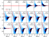 |
Fig. 3 Departure coefficients for the lowest 17 LS terms of N I in order of increasing energy (from left to right, top to bottom), as well as the ground level of N I (final panel). The contours show the distributions in the 3D model solar atmosphere. The departure coefficients calculated in the ⟨3D⟩ and 1D models are overplotted. |
N I abundances inferred from different spectrum synthesis models.
3.2 Nature of the 3D effect
To aid our understanding, it is useful to disentangle the 3D effect on spectral line formation into two separate effects: the direct effect, due to the granulation (Nordlund et al. 2009) that is present in the 3D model solar atmosphere but absent in the ⟨3D⟩ models, andthe indirect effect, due to differences in the atmospheric mean stratification between the ⟨3D⟩ model, and 1D models. In the Sun, the N I lines are susceptible to both types of 3D effects. They work in competition, however, as we explain below.
We investigate the direct 3D effect by illustrating in Fig. 4 the contribution function of a typical N I line in a vertical slice of a snapshot of the 3D model solar atmosphere. The N I lines considered in this study are all of rather high excitation energy. They thus preferentially form in high temperature regions: in the deep atmosphere log τR ≈ 0, and in the hot upflowing granules, rather than in the cool intergranular lanes. This can be seen in Fig. 4: as expected, the contribution function is largest (brightest, in the figure) in the deep atmosphere around the bumps in the contours of equal optical depth, which trace the solar granulation. As also seen for the outer wings of the Balmer lines of high excitation energy (see Fig. 2 of Amarsi et al. 2018b), this direct 3D effect acts to strengthen the N I lines, due to the granulestypically having steeper vertical temperature gradients than compared to the mean temperature structure.
Although the N I line formation is biased towards the granules in the deep atmosphere − 0.2 ≲ log τR ≲ 0.7, some additional line formation does occur in the upper atmosphere. Figure 4 reveals that even at log τR ≈−1 to − 2, minor line formation can occur in the hot temperature regions above the intergranular lanes (in the reversed granulation; Rutten et al. 2004), for example at x ≈ 1.5 Mm, 0.1 ≲height ≲ 0.5 Mm. Moreover, in this particular plot a blob of hot gas at x ≈ 2.5 Mm, height ≈ 0.8 Mm (log τR < −4) is apparent. Some line formation occurs here as well, although it is three orders of magnitude less efficient than the line formation in the solar granulation in the deep atmosphere.
These two direct 3D effects, namely N I line formation in the solar granules, and extended line formation in the upper atmosphere, both act to strengthen the N I lines and thus reduce the abundances inferred from the 3D model. This can be seen in Table 3, where the 3D non-LTE − ⟨3D⟩ non-LTE abundance difference is − 0.05 dex, averaged over the five N I lines. The direct effect occurs in regions of higher gas temperature, and consequently the abundance difference is largest for the lines of higher excitation energy, namely the N I 863 nm and 1011 nm lines (around − 0.06 dex), compared to the weaker lines (− 0.04 dex).
The nature of the indirect 3D effect can be seen in Fig. 1. There are differences between the mean temperature stratification of the 3D model (traced by the ⟨3D⟩ model) and that of the 1D model. At log τR = 0.5 the 1D model is about 150 K hotter, and at log τR = −0.5 the 1D model is about 75 K cooler. Thus in the N I line forming regions the ⟨3D⟩ model has a much shallower temperature gradient than the 1D model. The indirect 3D effect acts to weaken the N I lines, leading to higher abundances inferred in the 3D model compared to in the 1D model.
The indirect 3D effect is weaker than the direct 3D effect. This can be seen in Table 3, where the ⟨3D⟩ non-LTE − 1D non-LTE abundance difference is only + 0.01 dex, averaged over the five N I lines. Consequently the overall 3D effect is dominated by the direct effect, and the 3D non-LTE − 1D non-LTE abundance difference is negative: − 0.04 dex, again averaged over the five N I lines.
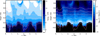 |
Fig. 4 Gas temperature (left) and line forming regions for the N I 868 nm line (right) in a vertical slice of a snapshot of the 3D model solar atmosphere. The latter quantity is based on the line-integrated contribution function to the line depression in the disk-centre intensity (Eq. (15) of Amarsi 2015). Contours of constant log τR are overplotted. |
3.3 3D/non-LTE coupling
It is interesting to briefly consider how the non-LTE effects discussed in Sect. 3.1, couple to the 3D effects discussed in Sect. 3.2. To quantify this 3D/non-LTE coupling, we compare the line-by-line non-LTE versus LTE abundance differences in Table 3 to each other. The [3D non-LTE − 3D LTE] − [1D non-LTE − 1D LTE] abundance difference, is insignificant: − 0.004 dex, averaged over the five N I lines. This coupling is even smaller if the indirect 3D effect is omitted, by considering the [3D non-LTE − 3D LTE] − [⟨3D⟩ non-LTE − ⟨3D⟩ LTE] abundance difference: − 0.002 dex, again averaged over the five N I lines.
The reason for the small 3D/non-LTE coupling can be seen in Fig. 3. The panels show that, in the N I line forming regions − 0.2 ≲ log τR ≲ 0.7, the departure coefficients calculated for different levels in the ⟨3D⟩ and 1D model solar atmospheres closely follow each other, and also follow the median of the corresponding distributions in the 3D model. They only begin to deviate from each other higher up in the atmosphere, at log τR ≲−3; here, the ⟨3D⟩ results follow the 3D distribution more closely than the 1D results.
Thus, the 3D/non-LTE coupling is not very severe for N I in the Sun. We caution, however, that this result does not necessarily extend to all late-type stars. The Sun has a very stratified atmosphere compared to other late-type stars, and the coupling is likely to be larger for stars with stronger granulation contrast; namely, for hotter, and more metal-poor stars.
4 The solar nitrogen abundance
4.1 Advocated abundance and uncertainty
Our recommended solar nitrogen abundance from N I lines is log ɛN = 7.77 ± 0.05. This value is determined from the unweighted mean from the five N I lines given by the 3D non-LTE model (Table 3), and is based on fitting the deblended equivalent widths that were measured at solar disk centre (Table 2).
The 3D non-LTE abundance inferred here is lower than that inferred from the 3D LTE model, and from the ⟨3D⟩ and 1D models in both non-LTE and LTE. Both the non-LTE effect (Sect. 3.1) and the 3D effect (Sect. 3.2) strengthen the N I lines. Therefore the 3D non-LTE abundance corrections are negative, relative to the various ⟨3D⟩, 1D, and LTE models in Table 3.
The line-by-line dispersion is low, corresponding to a standard error of 0.002 dex for the 3D non-LTE model (Table 3). We thus assume that the overall uncertainty is dominated by systematics.
To estimate systematic errors arising from the measurement of the deblended equivalent widths of the N I lines, the abundance analysis was repeated using the older estimates for the equivalent widths given in Grevesse et al. (1990). This same set of equivalent widths was used in the abundance analysis of Caffau et al. (2009). These equivalent widths are systematically somewhat larger: the differences in the inferred abundances range from 0.02 dex larger (N I 868 nm) to 0.11 dex larger (N I 1011 nm); the mean difference is 0.057 dex.
Following Scott et al. (2015) we combine, in quadrature, half of this difference due to the equivalent widths (0.028 dex), with: (a) half the difference between the 3D and ⟨3D⟩ results, to quantify the uncertainty in the direct 3D effect (0.025 dex); (b) half the difference between the ⟨3D⟩ and 1D results, to quantify the uncertainty in the indirect 3D effect (0.006 dex); and (c) half the difference between the non-LTE and LTE results, to quantify the uncertainty in the non-LTE effect (0.007 dex). We also fold in the uncertainty in the oscillator strengths, taken to be 0.03 dex based on their B+/B rankings given on NIST (Kramida et al. 2012). This gives the final result of 0.05 dex.
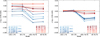 |
Fig. 5 Difference between Caffau et al. (2009) and this work, after adopting the line selection and identical equivalent widths (Grevesse et al. 1990), for different spectrum synthesis models. The three lines in common between that study and the present one are marked in parentheses. The right panel shows the differences after correcting the abundances for the differences in log gf between the two studies. |
4.2 Comparison with Caffau et al. (2009)
Our advocated result, log ɛN = 7.77 ± 0.05, is somewhat lower than that presented in Caffau et al. (2009), namely log ɛN = 7.86 ± 0.12. That study and the present one are both based purely on N I lines. Both are based on 3D radiative-hydrodynamic model atmospheres and non-LTE radiative transfer: however, the present study adopts a full 3D non-LTE approach, whereas their study adds non-LTE abundance corrections from their ⟨3D⟩ model solar atmosphere, to their 3D LTE abundances. Nevertheless, the 3D/non-LTE coupling effect is quite weak for N I in the Sun (Sect. 3.3). Consequently their “3D LTE + ⟨3D⟩ non-LTE” approximation should be in good agreement with the full 3D non-LTE approach.
The main differences between the present study and that of Caffau et al. (2009) are in the N I line selection and the adopted equivalent widths. Caffau et al. (2009) include twelve N I lines, compared to five in the present study. The two studies have just three lines in common: the N I 744, 822, and 868 nm lines. As we discussed in Sect. 2.1, a restrictive line selection was adopted here based on analysing very carefully line shapes, in order to minimise the impact of unidentified blends that tend to skew the inferred abundances upwards. Moreover, Caffau et al. (2009) adopt the de-blended equivalent widths from Grevesse et al. (1990); these values tend to be systematically larger than those advocated in this study (Sect. 4.1). This amounts to an abundance difference of 0.06 dex for the five N I lines in Table 1.
We illustrate line-by-line abundance differences between the present study and that of Caffau et al. (2009), in the left panel of Fig. 5. The plot includes the twelve N I lines from their study and is based on their adopted equivalent widths. The line parameters adopted in the present study (Sect. 2.4), are slightly different to those adopted in Caffau et al. (2009). In the right panel of the figure we show the same abundance differences after correcting for the differences in the adopted oscillator strengths: Δ log gf = −Δlog ɛN.
The right panel of Fig. 5 shows that the 3D LTE and ⟨3D⟩ LTE results from this study and from Caffau et al. (2009) are in remarkable agreement, after correcting for differences in the adopted equivalent widths and line parameters. It is clear, however, that there are differences between the two studies, originating from differences in the non-LTE modelling. For the three lines in common between the two studies, these differences reach almost − 0.03 dex. The main uncertainty in the non-LTE model atom is perhaps the hydrogen collisions (Sect. 4.3). Caffau et al. (2009) adopt the Drawin recipe for these processes, employing a fudge factor of SH = 1∕3. While this was perhaps the best available approach at the time, it is now known that the Drawin recipe does not describe the correct underlying physical mechanism of these processes (Barklem et al. 2011). The non-LTE model atom presented here uses instead the LCAO/free electron method. We have previously argued that this more accurately represents reality, on the basis of both physical principles, and empirical results (Amarsi et al. 2018a, 2019).
Adopting the same twelve N I lines and using identical oscillator strengths and equivalent widths as Caffau et al. (2009), we obtain log ɛN = 7.87. This is in almost perfect agreement with their result, including a similarly large standard deviation in the results of 0.11 dex that suggests neglected blends and deficiencies in the adopted equivalent widths. We conclude that this is the main reason for the 0.09 dex larger abundance inferred by Caffau et al. (2009). While differences in the non-LTE modelling also play a small role (of the order 0.03 dex), differences between the two 3D model solar atmospheres appear not to contribute significantly to this discrepancy.
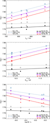 |
Fig. 6 Abundances inferred from the five N I lines in Table 1, using the equivalent widths measured at solar disk centre given in Table 2. Symbols indicate results from the different spectrum synthesis models. The least squares regressions for each model are overplotted. |
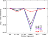 |
Fig. 7 Difference in the inferred abundances when switching off the specified ingredients in the non-LTE model atom: from left to right, fine structure; excitation of N I via electron collisions (Eq. (1)); ionisation of N I via electron collisions (Eq. (2)); excitation of N I via hydrogen collisions (Eq. (3)); charge transfer of N I via hydrogen collisions (Eq. (4); and ionisation of N I via hydrogen collisions (Eq. (5)). These results are based on the standard non-LTE model atom, and using the 1D model solar atmosphere. |
4.3 Model dependence
We illustrate the line-by-line abundances as functions of different line parameters in Fig. 6, for the different spectrum synthesis models. The ⟨3D⟩ and 1D models give rise to clear trends in the inferred abundances with respect to the wavelength, excitation energy, and reduced equivalent width. These trends are largely driven by the strong direct 3D effect on the N I lines, that is due to the solar granulation (Sect. 3.2). These trends are also reflected in the relatively large standard errors in Table 3 from these models.
The flat trends given by the 3D non-LTE and 3D LTE models in Fig. 6, and the smaller standard errors given in Table 3, is strong support of the reliability of the 3D model solar atmosphere used in the present work, at least in the deep layers where the N I lines form, − 0.2 ≲ log τR ≲ 0.7. This result, combined with previous scrutiny of the present 3D model (Sect. 2.1.4 of Amarsi et al. 2018a), and the excellent agreement between the 3D LTE results of the present study with the 3D LTE results of Caffau et al. (2009) based on an independent CO5BOLD simulation (when using identical oscillator strengths and equivalent widths; Sect. 4.2), all suggest that uncertainties in the 3D radiative-hydrodynamic simulations do not have a significant impact on the error budget in the present study (Sect. 4.1).
We test the sensitivity of the inferred abundances to different ingredients in the non-LTE model atom in Fig. 7. As found for C I (see Fig. 5 of Amarsi et al. 2019), the non-LTE results appear to be most sensitive to the inelastic collisions with neutral hydrogen that lead to excitation of N I. In the most extreme case, for the N I 868 nm line, the inferred abundance changes by almost 0.03 dex when hydrogen collisions are switched off; the mean difference for the five N I lines is 0.02 dex. It is interesting that the N I 1011 nm line clearly has a lower sensitivity to the hydrogen collisions than the other four lines: this likely reflects that the line is the least sensitive to departures from LTE in general, owing to the competing non-LTE effects on it (Sect. 3.1).
Figure 7 shows that the hydrogen collisions play an important role in the non-LTE modelling. We have previously motivated our combined LCAO/free electron method employed here, by studying the centre-to-limb variation of lines of O I (Amarsi et al. 2018a) and C I (Amarsi et al. 2019). If the hydrogen collisions are the largest uncertainty in the non-LTE model atom, this places an upper bound of 0.02 dex on the uncertainty that propagates to the inferred solar nitrogen abundance.
5 Conclusion
We present an analysis of the solar photospheric nitrogen abundance, employing a full 3D non-LTE approach, and a model atom that uses physically-motivated descriptions for the inelastic collisions between N I and free electrons, and between N I and neutral hydrogen. We dissected the line formation properties of the N I lines, explaining how both non-LTE photon losses, and 3D granulation effects, both act to reduce the abundances inferred from the N I lines of high excitation energy, by around 0.01 dex and 0.04 dex respectively. Our advocated value is log ɛN = 7.77 ± 0.05.
There iscurrently an exceptional interest in revisiting the solar elemental composition, because of the long-standing solar modelling problem. Standard solar interior models fail to reproduce several observational constraints precisely determined from helioseismology (e.g. Basu & Antia 2008). It has been noted in the literature that replacing the standard set of solar abundances of Asplund et al. (2009), with the older canonical compilations of Anders & Grevesse (1989), Grevesse & Noels (1993), or Grevesse & Sauval (1998), would help resolve the problem. However, new analyses suggest that the origin of thediscrepancy is more complex than simply the adopted solar abundances (Bailey et al. 2015; Buldgen et al. 2019).
It is thus important to verify that the standard set of solar abundances are indeed robust. For nitrogen, our advocated value of log ɛN = 7.77 ± 0.05 is in excellent agreement with that presented by Asplund et al. (2009) from N I lines, namely log ɛN = 7.78 ± 0.05. However, it is slightly lower than the standard value that they advocate, namely log ɛN = 7.83 ± 0.05. This latter value is larger because it folds in results from the NH rotational-vibrational lines (Δν = 1), from which Asplund et al. (2009) obtain log ɛN = 7.88 ± 0.03. This discrepancy between the atomic and molecular diagnostics of more than 0.1 dex is a cause of some concern. New molecular data that are available for NH (Brooke et al. 2014a, 2015) and CN (Brooke et al. 2014b), as well as updates to the 3D model atmosphere, may well be enough to resolve the discrepancy. This should be addressed in a future study.
Acknowledgements
We thank the anonymous referee for their helpful suggestions. A.M.A., P.S.B., and J.G. acknowledge support from the Swedish Research Council (VR 2016-03765), and the project grants “The New Milky Way” (KAW 2013.0052) and “Probing charge- and mass- transfer reactions on the atomic level” (KAW 2018.0028) from the Knut and Alice Wallenberg Foundation. M.A. gratefully acknowledges funding from the Australian Research Council (grants DP150100250 and FL110100012). Funding for the Stellar Astrophysics Centre is provided by The Danish National Research Foundation (grant DNRF106). Some of the computations were performed on resources provided by the Swedish National Infrastructure for Computing (SNIC) at the Multidisciplinary Center for Advanced Computational Science (UPPMAX) and at the High Performance Computing Center North (HPC2N) under project SNIC 2019/3-532. This work was supported by computational resources provided by the Australian Government through the National Computational Infrastructure (NCI) under the National Computational Merit Allocation Scheme.
References
- Allen, C. W. 1973, Astrophysical Quantities, 3rd edn. (London: University of London, Athlone Press) [Google Scholar]
- Amarsi, A. M. 2015, MNRAS, 452, 1612 [NASA ADS] [CrossRef] [Google Scholar]
- Amarsi, A. M., & Asplund, M. 2017, MNRAS, 464, 264 [NASA ADS] [CrossRef] [Google Scholar]
- Amarsi, A. M., & Barklem, P. S. 2019, A&A, 625, A78 [NASA ADS] [CrossRef] [EDP Sciences] [Google Scholar]
- Amarsi, A. M., Lind, K., Asplund, M., Barklem, P. S., & Collet, R. 2016, MNRAS, 463, 1518 [NASA ADS] [CrossRef] [Google Scholar]
- Amarsi, A. M., Barklem, P. S., Asplund, M., Collet, R., & Zatsarinny, O. 2018a, A&A, 616, A89 [NASA ADS] [CrossRef] [EDP Sciences] [Google Scholar]
- Amarsi, A. M., Nordlander, T., Barklem, P. S., et al. 2018b, A&A, 615, A139 [NASA ADS] [CrossRef] [EDP Sciences] [Google Scholar]
- Amarsi, A. M., Barklem, P. S., Collet, R., Grevesse, N., & Asplund, M. 2019, A&A, 624, A111 [NASA ADS] [CrossRef] [EDP Sciences] [Google Scholar]
- Anders, E., & Grevesse, N. 1989, Geochim. Cosmochim. Acta, 53, 197 [Google Scholar]
- Anstee, S. D., & O’Mara, B. J. 1995, MNRAS, 276, 859 [NASA ADS] [CrossRef] [Google Scholar]
- Asplund, M., Nordlund, Å., Trampedach, R., Allende Prieto, C., & Stein, R. F. 2000, A&A, 359, 729 [NASA ADS] [Google Scholar]
- Asplund, M., Grevesse, N., Sauval, A. J., & Scott, P. 2009, ARA&A, 47, 481 [NASA ADS] [CrossRef] [Google Scholar]
- Bailey, J. E., Nagayama, T., Loisel, G. P., et al. 2015, Nature, 517, 56 [NASA ADS] [CrossRef] [Google Scholar]
- Barklem, P. S. 2016a, A&ARv, 24, 9 [NASA ADS] [CrossRef] [Google Scholar]
- Barklem, P. S. 2016b, Phys. Rev. A, 93, 042705 [NASA ADS] [CrossRef] [Google Scholar]
- Barklem, P. S. 2017, Astrophysics Source Code Library [record ascl:1701.005] [Google Scholar]
- Barklem, P. S., & O’Mara, B. J. 1997, MNRAS, 290, 102 [Google Scholar]
- Barklem, P. S., O’Mara, B. J., & Ross, J. E. 1998, MNRAS, 296, 1057 [Google Scholar]
- Barklem, P. S., Belyaev, A. K., Guitou, M., et al. 2011, A&A, 530, A94 [NASA ADS] [CrossRef] [EDP Sciences] [Google Scholar]
- Basu, S., & Antia, H. M. 2008, Phys. Rep., 457, 217 [NASA ADS] [CrossRef] [Google Scholar]
- Belfiore, F., Maiolino, R., Tremonti, C., et al. 2017, MNRAS, 469, 151 [NASA ADS] [CrossRef] [Google Scholar]
- Bell, K. L., & Berrington, K. A. 1991, J. Phys., 24, 933 [NASA ADS] [Google Scholar]
- Belyaev, A. K. 2013, Phys. Rev. A, 88, 052704 [NASA ADS] [CrossRef] [Google Scholar]
- Berg, D. A., Erb, D. K., Henry, R. B. C., Skillman, E. D., & McQuinn, K. B. W. 2019, ApJ, 874, 93 [NASA ADS] [CrossRef] [Google Scholar]
- Biémont, E., Froese Fischer, C., Godefroid, M., Vaeck, N., & Hibbert, A. 1990, in 3rd International Collogium of the Royal Netherlands Academy of Arts and Sciences, 59 [Google Scholar]
- Böhm-Vitense, E. 1958, Z. Astrophys., 46, 108 [Google Scholar]
- Brooke, J. S. A., Bernath, P. F., Western, C. M., van Hemert, M. C., & Groenenboom, G. C. 2014a, J. Chem. Phys., 141, 054310 [NASA ADS] [CrossRef] [Google Scholar]
- Brooke, J. S. A., Ram, R. S., Western, C. M., et al. 2014b, ApJS, 210, 23 [NASA ADS] [CrossRef] [Google Scholar]
- Brooke, J. S. A., Bernath, P. F., & Western, C. M. 2015, J. Chem. Phys., 143, 026101 [NASA ADS] [CrossRef] [Google Scholar]
- Buldgen, G., Salmon, S. J. A. J., Noels, A., et al. 2019, A&A, 621, A33 [NASA ADS] [CrossRef] [EDP Sciences] [Google Scholar]
- Caffau, E., Maiorca, E., Bonifacio, P., et al. 2009, A&A, 498, 877 [NASA ADS] [CrossRef] [EDP Sciences] [Google Scholar]
- Collet, R., Nordlund, Ã., Asplund, M., Hayek, W., & Trampedach, R. 2018, MNRAS, 475, 3369 [NASA ADS] [CrossRef] [Google Scholar]
- Cunto, W., Mendoza, C., Ochsenbein, F., & Zeippen, C. J. 1993, A&A, 275, L5 [NASA ADS] [Google Scholar]
- Delbouille, L., & Roland, C. 1995, ASP Conf. Ser., 81, 32 [NASA ADS] [Google Scholar]
- Delbouille, L., Roland, G., & Neven, L. 1973, Atlas Photometrique Du Spectre Solaire De [lambda] 3000 a [lambda] 10000 (Liège: Université de Liège, Institut d’Astrophysique) [Google Scholar]
- Drawin, H.-W. 1968, Z. Phys., 211, 404 [NASA ADS] [CrossRef] [EDP Sciences] [Google Scholar]
- Drawin, H. W. 1969, Z. Phys., 225, 483 [NASA ADS] [CrossRef] [EDP Sciences] [Google Scholar]
- Esteban, C., & García-Rojas, J. 2018, MNRAS, 478, 2315 [NASA ADS] [CrossRef] [Google Scholar]
- Freytag, B., Steffen, M., Ludwig, H.-G., et al. 2012, J. Comput. Phys., 231, 919 [Google Scholar]
- Froese Fischer, C. 1997, Computational Atomic Structure : An MCHF Approach (Abingdon-on-Thames, UK: Routledge) [Google Scholar]
- Froese Fischer, C. 2000, Comput. Phys. Commun., 128, 635 [NASA ADS] [CrossRef] [Google Scholar]
- Froese Fischer, C., Tachiev, G., Gaigalas, G., & Godefroid, M. R. 2007, Comput. Phys. Commun., 176, 559 [NASA ADS] [CrossRef] [Google Scholar]
- Froese Fischer, C., Godefroid, M., Brage, T., Jönsson, P., & Gaigalas, G. 2016, J. Phys., 49, 182004 [Google Scholar]
- Froese Fischer, C., Gaigalas, G., Jönsson, P., & Bieroń, J. 2019, Comput. Phys. Commun., 237, 184 [NASA ADS] [CrossRef] [Google Scholar]
- Gray, D. F. 2008, The Observation and Analysis of Stellar Photospheres (Cambridge: Cambridge University Press) [Google Scholar]
- Grevesse, N., & Noels, A. 1993, in Origin and Evolution of the Elements, eds. N. Prantzos, E. Vangioni-Flam, & M. Casse (Singapore: World Scientific), 15 [Google Scholar]
- Grevesse, N., & Sauval, A. J. 1998, Space Sci. Rev., 85, 161 [NASA ADS] [CrossRef] [Google Scholar]
- Grevesse, N., Lambert, D. L., Sauval, A. J., et al. 1990, A&A, 232, 225 [NASA ADS] [Google Scholar]
- Grevesse, N., Asplund, M., & Sauval, A. J. 2007, The Solar Chemical Composition, eds. R. von Steiger, G. Gloeckler, & G. M. Mason (Berlin: Springer Science+Business Media), 105 [Google Scholar]
- Gustafsson, B., Edvardsson, B., Eriksson, K., et al. 2008, A&A, 486, 951 [NASA ADS] [CrossRef] [EDP Sciences] [Google Scholar]
- Henyey, L., Vardya, M. S., & Bodenheimer, P. 1965, ApJ, 142, 841 [NASA ADS] [CrossRef] [Google Scholar]
- Hibbert, A., Biemont, E., Godefroid, M., & Vaeck, N. 1991, A&AS, 88, 505 [NASA ADS] [Google Scholar]
- Ibgui, L., Hubeny, I., Lanz, T., & Stehlé, C. 2013, A&A, 549, A126 [NASA ADS] [CrossRef] [EDP Sciences] [Google Scholar]
- Karakas, A. I., & Lattanzio, J. C. 2014, PASA, 31, e030 [NASA ADS] [CrossRef] [Google Scholar]
- Kaulakys, B. P. 1985, J. Phys., 18, L167 [NASA ADS] [Google Scholar]
- Kaulakys, B. P. 1986, JETP, 91, 391 [Google Scholar]
- Kaulakys, B. P. 1991, J. Phys., 24, L127 [Google Scholar]
- Kramida, A., Ralchenko, Y., Reader, J., et al. 2012, NIST atomic spectra database (version 5) [Google Scholar]
- Kramida, A., Yu. Ralchenko, Reader, J., & NIST ASD Team. 2015, NIST, NIST Atomic Spectra Database (ver. 5.3) [online], available: http://physics.nist.gov/asd [2015, November 2], National Institute of Standards and Technology, Gaithersburg, MD [Google Scholar]
- Lambert, D. L. 1993, Phys. Scr., 47, 186 [NASA ADS] [CrossRef] [Google Scholar]
- Leenaarts, J., & Carlsson, M. 2009, ASP Conf. Ser., 415, 87 [Google Scholar]
- Lodders, K. 2019, ArXiv e-prints [arXiv:1912.00844] [Google Scholar]
- Lyubimkov, L. S., Korotin, S. A., & Lambert, D. L. 2019, MNRAS, 489, 1533 [NASA ADS] [CrossRef] [Google Scholar]
- Magic, Z., Collet, R., Asplund, M., et al. 2013, A&A, 557, A26 [NASA ADS] [CrossRef] [EDP Sciences] [Google Scholar]
- Magrini, L., Vincenzo, F., Randich, S., et al. 2018, A&A, 618, A102 [NASA ADS] [CrossRef] [EDP Sciences] [Google Scholar]
- Martin, W. C., & Wiese, W. 1999, Atomic Spectroscopy: A Compendium of Basic Ideas, Notation, Data, and Formulas (Gaithersburg, USA: National Institute of Standards and Technology) [Google Scholar]
- Moore, C. E. 1993, Tables of Spectra of Hydrogen, Carbon, Nitrogen, and Oxygen Atoms and Ions, ed. J. Gallagher (Boca Raton, Florida: CRC press) [Google Scholar]
- Musielok, J., Wiese, W. L., & Veres, G. 1995, Phys. Rev. A, 51, 3588 [NASA ADS] [CrossRef] [PubMed] [Google Scholar]
- Neckel, H. 1999, Sol. Phys., 184, 421 [NASA ADS] [CrossRef] [Google Scholar]
- Neckel, H., & Labs, D. 1984, Sol. Phys., 90, 205 [NASA ADS] [CrossRef] [Google Scholar]
- Nordlund, Å., & Galsgaard, K. 1995, A 3D MHD code for Parallel Computers, Technical report rep., Niels Bohr Institute, University of Copenhagen [Google Scholar]
- Nordlund, Å., Stein, R. F., & Asplund, M. 2009, Liv. Rev. Sol. Phys., 6, 2 [Google Scholar]
- Rentzsch-Holm, I. 1996, A&A, 305, 275 [NASA ADS] [Google Scholar]
- Rutten, R. J. 2003, Radiative Transfer in Stellar Atmospheres, 8th edn. (Utrecht: Utrecht University) [Google Scholar]
- Rutten, R. J., de Wijn, A. G., & Sütterlin, P. 2004, A&A, 416, 333 [NASA ADS] [CrossRef] [EDP Sciences] [Google Scholar]
- Rybicki, G. B., & Hummer, D. G. 1992, A&A, 262, 209 [NASA ADS] [Google Scholar]
- Salgado, C., Da Costa, G. S., Norris, J. E., & Yong, D. 2019, MNRAS, 484, 3093 [NASA ADS] [CrossRef] [Google Scholar]
- Schiavon, R. P., Zamora, O., Carrera, R., et al. 2017, MNRAS, 465, 501 [NASA ADS] [CrossRef] [Google Scholar]
- Scott, P., Grevesse, N., Asplund, M., et al. 2015, A&A, 573, A25 [NASA ADS] [CrossRef] [EDP Sciences] [Google Scholar]
- Steenbock, W., & Holweger, H. 1984, A&A, 130, 319 [NASA ADS] [Google Scholar]
- Tachiev, G. I., & Froese Fischer, C. 2002, A&A, 385, 716 [NASA ADS] [CrossRef] [EDP Sciences] [Google Scholar]
- Takeda, Y., & Honda, S. 2005, PASJ, 57, 65 [NASA ADS] [Google Scholar]
- van Regemorter, H. 1962, ApJ, 136, 906 [NASA ADS] [CrossRef] [Google Scholar]
- Vincenzo, F., Belfiore, F., Maiolino, R., Matteucci, F., & Ventura, P. 2016, MNRAS, 458, 3466 [NASA ADS] [CrossRef] [Google Scholar]
- Wang, Y., Zatsarinny, O., & Bartschat, K. 2014, Phys. Rev. A, 89, 062714 [NASA ADS] [CrossRef] [Google Scholar]
- Zafar, T., Centurión, M., Péroux, C., et al. 2014, MNRAS, 444, 744 [NASA ADS] [CrossRef] [Google Scholar]
- Zatsarinny, O. 2006, Comput. Phys. Commun., 174, 273 [NASA ADS] [CrossRef] [Google Scholar]
- Zhu, Q., Bridges, J. M., Hahn, T., & Wiese, W. L. 1989, Phys. Rev. A, 40, 3721 [NASA ADS] [CrossRef] [PubMed] [Google Scholar]
 , where NA and
NH are the number densities of nuclei of element A and of hydrogen.
, where NA and
NH are the number densities of nuclei of element A and of hydrogen.
The CompAS GRASP repository: github.com/compas/grasp
All Tables
All Figures
|
Fig. 1 Temperatures as functions of Rosseland mean optical depth for the different model solar atmospheres considered in this study (top), and residual difference between the 1D and ⟨3D⟩ models (bottom). The optical depths corresponding to peak line formation as well as the interquartile ranges of the 5 N I lines are indicated; these values are based on the line-integrated contribution function to the line depression in the disk-centre intensity (Eq. (15) of Amarsi 2015), calculated using the ⟨3D⟩ model solar atmosphere. |
| In the text | |
|
Fig. 2 Grotrian diagrams for N I in the comprehensive starting non-LTE model atom (left), and in the resulting non-LTE model atom after reducing its complexity (right). Energy levels are indicated as short black horizontal lines; those levels for which fine structure is not resolved are indicated as short blue horizontal lines, and super levels are shown as long blue horizontal lines. All bound–bound radiative transitions considered in the non-LTE iterations are shown in grey. The five abundance indicators are labelled and marked specially in the right panel. |
| In the text | |
|
Fig. 3 Departure coefficients for the lowest 17 LS terms of N I in order of increasing energy (from left to right, top to bottom), as well as the ground level of N I (final panel). The contours show the distributions in the 3D model solar atmosphere. The departure coefficients calculated in the ⟨3D⟩ and 1D models are overplotted. |
| In the text | |
|
Fig. 4 Gas temperature (left) and line forming regions for the N I 868 nm line (right) in a vertical slice of a snapshot of the 3D model solar atmosphere. The latter quantity is based on the line-integrated contribution function to the line depression in the disk-centre intensity (Eq. (15) of Amarsi 2015). Contours of constant log τR are overplotted. |
| In the text | |
|
Fig. 5 Difference between Caffau et al. (2009) and this work, after adopting the line selection and identical equivalent widths (Grevesse et al. 1990), for different spectrum synthesis models. The three lines in common between that study and the present one are marked in parentheses. The right panel shows the differences after correcting the abundances for the differences in log gf between the two studies. |
| In the text | |
|
Fig. 6 Abundances inferred from the five N I lines in Table 1, using the equivalent widths measured at solar disk centre given in Table 2. Symbols indicate results from the different spectrum synthesis models. The least squares regressions for each model are overplotted. |
| In the text | |
|
Fig. 7 Difference in the inferred abundances when switching off the specified ingredients in the non-LTE model atom: from left to right, fine structure; excitation of N I via electron collisions (Eq. (1)); ionisation of N I via electron collisions (Eq. (2)); excitation of N I via hydrogen collisions (Eq. (3)); charge transfer of N I via hydrogen collisions (Eq. (4); and ionisation of N I via hydrogen collisions (Eq. (5)). These results are based on the standard non-LTE model atom, and using the 1D model solar atmosphere. |
| In the text | |
Current usage metrics show cumulative count of Article Views (full-text article views including HTML views, PDF and ePub downloads, according to the available data) and Abstracts Views on Vision4Press platform.
Data correspond to usage on the plateform after 2015. The current usage metrics is available 48-96 hours after online publication and is updated daily on week days.
Initial download of the metrics may take a while.