| Issue |
A&A
Volume 636, April 2020
|
|
|---|---|---|
| Article Number | A54 | |
| Number of page(s) | 26 | |
| Section | Stellar structure and evolution | |
| DOI | https://doi.org/10.1051/0004-6361/201936361 | |
| Published online | 17 April 2020 | |
VLT/X-shooter spectroscopy of massive young stellar objects in the 30 Doradus region of the Large Magellanic Cloud⋆,⋆⋆
1
Anton Pannekoek Institute, University of Amsterdam, Science Park 904, 1098 XH Amsterdam, The Netherlands
e-mail: This email address is being protected from spambots. You need JavaScript enabled to view it.
2
Leiden Observatory, Leiden University, PO Box 9513, 2300 RA Leiden, The Netherlands
3
Max-Plank-Institute for Astronomy, Königstuhl 17, 69117 Heidelberg, Germany
4
Departamento de Física y Astronomía, Universidad de La Serena, Av. cisternas 1200 Norte, La Serena, Chile
5
Department of Physics and Astronomy, University of Sheffield, Sheffield S3 7RH, UK
6
Department of Astronomy, Stockholm University, AlbaNova University Centre, 106 91 Stockholm, Sweden
7
Argelander-Institut für Astronomie der Universitét Bonn, Auf dem Hügel 71, 53121 Bonn, Germany
8
Institute of Astrophysics, KU Leuven, Celestijnenlaan 200D, 3001 Leuven, Belgium
9
Center for Astrophysics, Harvard-Smithsonian, 60 Garden Street, Cambridge, MA 02138, USA
10
Space Telescope Science Institute, 2700 San Martin Drive, Baltimore, MD 21218, USA
11
Department of Astronomy, University of Maryland, College Park, MD 20742, USA
12
CRESST II and Exoplanets and Stellar Astrophysics Laboratory, NASA Goddard Space Flight Center, Greenbelt, MD 20771, USA
13
Armagh Observatory, College Hill, Armagh BT61 9DG, UK
Received:
23
July
2019
Accepted:
6
February
2020
Abstract
The process of massive star (M ≥ 8 M⊙) formation is still poorly understood. Observations of massive young stellar objects (MYSOs) are challenging due to their rarity, short formation timescale, large distances, and high circumstellar extinction. Here, we present the results of a spectroscopic analysis of a population of MYSOs in the Large Magellanic Cloud. We took advantage of the spectral resolution and wavelength coverage of X-shooter (300−2500 nm), which is mounted on the European Southern Observatory Very Large Telescope, to detect characteristic spectral features in a dozen MYSO candidates near 30 Doradus, the largest starburst region in the Local Group hosting the most massive stars known. The X-shooter spectra are strongly contaminated by nebular emission. We used a scaling method to subtract the nebular contamination from our objects. We detect Hα, β, [O I] 630.0 nm, Ca II, infrared triplet [Fe II] 1643.5 nm, fluorescent Fe II 1687.8 nm, H2 2121.8 nm, Brγ, and CO bandhead emission in the spectra of multiple candidates. This leads to the spectroscopic confirmation of ten candidates as bona fide MYSOs. We compared our observations with photometric observations from the literature and find all MYSOs to have a strong near-infrared excess. We computed lower limits to the brightness and luminosity of the MYSO candidates, confirming the near-infrared excess and the massive nature of the objects. No clear correlation is seen between the Brγ luminosity and metallicity. Combining our sample with other LMC samples results in a combined detection rate of disk features, such as fluorescent Fe II and CO bandheads, which is consistent with the Galactic rate (40%). Most of our MYSOs show outflow features.
Key words: stars: formation / stars: pre-main sequence / stars: massive / HII regions / galaxies: clusters: individual: 30 Doradus / Magellanic Clouds
The full X-shooter spectra are only available at the CDS via anonymous ftp to cdsarc.u-strasbg.fr (130.79.128.5) or via http://cdsarc.u-strasbg.fr/viz-bin/cat/J/A+A/636/A54
Based on observations at the European Southern Observatory under ESO program 090.C-0346(A).
We regret to say that Dr. Nolan Walborn passed away early 2018. He was one of the initiators of this program.
© ESO 2020
1. Introduction
The formation process of massive stars (M ≥ 8 M⊙) is still poorly understood (e.g., Zinnecker & Yorke 2007; Beuther et al. 2007; Tan et al. 2014). Due to their short formation timescale (∼104−5 yr) and the severe extinction (AV ∼ 10−100 mag) by the surrounding gas and dust, observations of massive young stellar objects (MYSOs) are challenging. Additionally, massive stars are rare and therefore they are typically located at larger distances.
Already before reaching the zero-age main sequence (ZAMS), a MYSO is expected to produce significant amounts of ultraviolet (UV) radiation, creating an expanding hyper- or ultra-compact H II region (Churchwell 2002). Despite the strong UV radiation counteracting the accretion process through, for example, radiation pressure or photo-ionization (e.g., Wolfire & Cassinelli 1987; Krumholz et al. 2009; Kuiper et al. 2011; Kuiper & Hosokawa 2018), the current belief is that mass accretes onto the central (proto-)star via an accretion disk that is similar to low-mass stars.
If most of the mass is accreted through an accretion disk, MYSOs are expected to be surrounded by massive, extended disks (Beltrán & de Wit 2016). These disks have been observed spectroscopically around low, M ≲ 2 M⊙, and intermediate, 2 ≲ M ≲ 8 M⊙, mass stars (e.g., Ellerbroek et al. 2011; Alcalá et al. 2014). At near-infrared (NIR) wavelengths, disks around MYSOs are commonly observed (e.g., Bik et al. 2006; Wheelwright et al. 2010; Ilee et al. 2013), and disks around MYSOs have recently been detected at submillimeter and centimeter wavelengths (e.g., Ilee et al. 2016, 2018a). However, observations in the optical are scarce due to the high extinction. In the Galactic open cluster M17, Ramírez-Tannus et al. (2017) identified a population of MYSOs with disks by observing strong infrared excess and detecting double-peaked spectral lines in the optical. Additionally, they saw CO bandhead emission, which can be produced in a Keplerian disk (e.g., Blum et al. 2004; Bik & Thi 2004; Bik et al. 2006; Wheelwright et al. 2010; Ilee et al. 2013) and seems to be highly dependent on the accretion rate (Ilee et al. 2018b). The Galactic Red MSX Source (RMS) survey has shown that the luminosity of accretion tracers, such as Brγ, is correlated to the mass of the YSO and that disk tracing features, such as CO bandheads and fluorescent Fe II emission, are present in ∼40% of the MYSOs (Cooper et al. 2013; Pomohaci et al. 2017).
Outflows are common in MYSOs (e.g., Zhang et al. 2001, 2005). In the earliest stage of star formation, they are mostly molecular in origin (Bachiller 1996). At later stages, the outflow contains low-density atomic material and hence shows forbidden lines of O, N, S, or Fe, for instance, which are either ionized or not (Ellerbroek et al. 2013a). Additionally, the [O I] 630.0 nm line has been observed to originate from disk winds or the regions where the stellar UV radiation impinges on the disk surface (e.g., Finkenzeller 1985; van der Plas et al. 2008).
The Magellanic Clouds are interesting systems for studying massive star formation. The lower metallicity in the Large Magellanic cloud (LMC) and Small Magellanic Cloud (SMC, about 1/2 and 1/5 of solar, respectively; Peimbert et al. 2000; Rolleston et al. 2002) may influence the process of massive star formation. Most spectroscopic observations of MYSOs in the LMC and SMC have been in the mid-infrared (MIR) with the Spitzer/Infrared Spectrograph (IRS; e.g., van Loon et al. 2005; Oliveira et al. 2009, 2013; Seale et al. 2009, 2011; Woods et al. 2011; Ruffle et al. 2015; Jones et al. 2017). In the NIR, MYSOs in the LMC have also been observed by the AKARI Infrared Camera (Shimonishi et al. 2008, 2010). The Very Large Telescope (VLT) allow us now to spectroscopically observe apparent single MYSOs in the Magellanic Clouds (e.g., Ward et al. 2016, 2017; Ward 2017; Rubio et al. 2018; Reiter et al. 2019).
30 Doradus (30 Dor; also known as the Tarantula Nebula) is the most prominent massive star forming region in the Local Group. It is situated in the LMC at a distance of about 50 kpc (Pietrzyński et al. 2013). Its dense massive core, Radcliffe 136 (R136), has a total mass of up to 105 M⊙ and a cluster age of ∼1.5 Myr (Selman & Melnick 2013; Crowther et al. 2016). R136 hosts the most massive stars known with masses up to 300 M⊙ (de Koter et al. 1997; Crowther et al. 2010). The strong UV radiation originating from the hot stars in R136 ionizes the surrounding cluster medium, creating the largest H II region of the LMC and the Local Group in general. Recent initial mass function (IMF) measurements show 30 Dor to host an excess of about 30% in massive stars compared to the Salpeter IMF (Salpeter 1955; Schneider et al. 2018a). 30 Dor has been observed extensively in the VLT/FLAMES Tarantula Survey by obtaining high resolution spectra of about 800 O and B stars (Evans et al. 2011), and in the Hubble Tarantula Treasury Project (HTTP), a panchromatic imaging survey with Hubble Space Telescope (HST) of 30 Dor’s stellar population down to masses of 0.5 M⊙ (Sabbi et al. 2013, 2016).
The massive star formation rate in 30 Dor apparently rapidly increased about 7−8 Myr ago (Cignoni et al. 2015; Schneider et al. 2018b), but it seems to have diminished about 1 Myr ago (though this may be an extinction effect; heavily extincted stars are not in the VFTS and HTTP samples). Nevertheless, in the nebular region surrounding R136, ongoing massive star formation has been suggested. Hyland et al. (1992) observed four candidate protostars with masses of 15−20 M⊙ and Rubio et al. (1992) discovered 17 NIR sources to the north and west of R136. Later investigations showed 30 Dor to be a two-stage starburst region (Walborn & Parker 1992), with substantial star formation going on in the surrounding region (Walborn et al. 1999; Brandner et al. 2001). More recently, Walborn et al. (2013) reported the top ten MYSO candidates using the Spitzer/InfraRed Array Camera (IRAC) 3−8 μm wavelength range from the Surveying the Agents of a Galaxy’s Evolution (SAGE; Meixner et al. 2006) program combined with the Visible and Infrared Survey Telescope for Astronomy Magellanic Survey (VMC; Cioni et al. 2011) photometric observations. They derived masses and luminosities of about 10−30 M⊙ and 104−5 L⊙, respectively, by fitting the spectral energy distribution (SED) to the YSO models of Robitaille et al. (2006). Additionally, they conclude that all apparently single MYSO candidates are Class I sources (using the classification scheme based on the MIR spectral index of Andre et al. 2000). Throughout this paper, we refer to the empirically defined Classes and Types (based on the appearance of the SED; Chen et al. 2009) and the theoretically defined Stages of Robitaille et al. (2006). Since Class 0 objects may only be distinguished from Class I objects at submillimeter wavelengths, we combine these as Class 0/I.
In this paper, we report the results of optical (300 nm) to NIR (2500 nm) follow-up observations with VLT/X-shooter (Vernet et al. 2011) of the top ten Spitzer MYSO candidates of Walborn et al. (2013). The aim is to confirm their MYSO nature using optical and NIR emission features. In Sect. 2 we introduce the target sample and photometry from the literature. Our VLT/X-shooter observations, data reduction, and methods of subtracting nebular contamination are described in Sect. 3. Our analysis of the spectra and classification of the targets, leading to the confirmation of ten candidates as MYSOs, are presented in Sect. 4. We discuss the results in Sect. 5. Section 6 provides a summary.
2. Target sample
2.1. Target selection
Our targets were selected based on the top ten MYSO candidates of Walborn et al. (2013). They selected the ten brightest targets in the Spitzer/IRAC bands (labeling them as S1–S10) and combined these with VMC photometry. In this work, we adopt the same names. In Fig. 1 we show the positions of our targets in a VMC Y (1.02 μm), J (1.25 μm), and Ks (2.15 μm) three-color image. In the VLT/X-shooter observation of S5, a total of six objects could be identified within the slit range, which we labeled S5-A, B, C, D, E, and F (see Fig. 8). S8 is an unresolved double-system, which we discuss as one single target. S10-B and S10-C are also unresolved and are labeled as S10-BC in this work. Supplementary to S1–S10 and additional targets on the slit, our target sample includes R135; a WR star of spectral type (SpT) WN7h+OB (Evans et al. 2011) located in the vicinity of S3 and S3-K. A log of our VLT/X-shooter observations of a total of 23 sources is presented in Table 1.
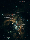 |
Fig. 1. 30 Dor nebula seen in the Y (blue), J (green), and Ks (red) bands with the VMC (Cioni et al. 2011). North is up and east is to the left. The observed X-shooter targets are labeled in white (see also Table 1). The central massive cluster R136 is the bright cluster of stars in the middle. |
VLT/X-shooter observations used in this paper.
2.2. Photometry
With the Visible and Infrared Survey Telescope for Astronomy (VISTA) IR camera (Dalton et al. 2006) J-band and Ks-band and Infrared Survey Facility (IRSF; Kato et al. 2007) H-band (1.63 μm) photometric observations presented by Walborn et al. (2013), we constructed a NIR color-magnitude and color-color diagram of our targets; see Fig. 2. For S5-A and R135, all magnitudes are from the Two Micron All Sky Survey (2MASS; Cutri et al. 2003). We assumed a J > 19 lower limit for S3, S9, and S10-BC. We lack part of the relevant photometric observations of S1-SE, S5-B, S5-C, S5-D, and S5-F, hence these objects do not appear in Fig. 2. The ZAMS is computed using MESA Isochrones and Stellar Tracks (MIST) models (Paxton et al. 2011, 2013, 2015; Dotter 2016; Choi et al. 2016) with half the solar metallicity (Rolleston et al. 2002) and a distance to the LMC of 50 kpc (Pietrzyński et al. 2013). We also plotted the positions of O V stars of Martins & Plez (2006). Using the Maíz Apellániz et al. (2014) extinction law for 30 Dor, we drew the reddening lines of an O3 V star for a total-to-selective extinction RV of 3.1 (average Galactic value) and 5.0 (values observed in 30 Dor, e.g., Bestenlehner et al. 2011, 2014).
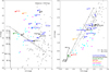 |
Fig. 2. Left: NIR color-magnitude diagram of our targets. With dots, we show the objects with accurate photometry (Cutri et al. 2003; Walborn et al. 2013) and, with arrows, we show the positions of objects based on a J > 19 lower limit. Errors on the data points were omitted for clarity but are typically ∼0.05 mag. In blue, we show the MYSOs confirmed in this work and, in black, the unconfirmed MYSO candidates. The green, red, and yellow dots indicate a MS, M-type giant, and WR star, respectively. The magenta dots are other LMC MYSOs (Ward et al. 2016; Reiter et al. 2019) and the cyan dots are SMC MYSOs (Ward et al. 2017; Rubio et al. 2018). The gray stars, squares, and diamonds are the MYSOs of Ramírez-Tannus et al. (2017), Bik et al. (2006), and Cooper et al. (2013) projected at a distance of 50 kpc, respectively. The ZAMS is shown as a black line, and the gray line indicates the position of O V stars of Martins & Plez (2006). The dashed black and gray lines are the reddening lines of an O3 V star for a RV of 3.1 and 5.0, respectively, where the crosses from left to right represent a visual extinction AV of 5, 10, 15, 20, 25, and 30 mag. We note that almost all our MYSO candidates are located above the reddening lines, implying a strong NIR excess. Right: NIR color-color diagram of our targets. The colors and symbols are the same as in the left plot. Most of our targets show evidence of a NIR excess due to their position at the right of the reddening lines. |
Almost all our MYSO candidates are located far above the reddening line for an O3 V star, indicating the presence of a strong NIR excess. For our brightest Ks-band target, S4, this excess may be ≳5 mag, suggesting the object to be ≳100 times brighter in the Ks-band than the central (proto)star would be. The NIR excess is considerably stronger compared to Galactic MYSO observations of Bik et al. (2006) and Ramírez-Tannus et al. (2017). Our sources have, on average, a bluer J − K color and brighter Ks-band magnitude than most objects in the sample of Cooper et al. (2013). This is an observational bias; our targets were selected as the brightest NIR and MIR targets in 30 Dor.
In star forming regions, the extinction is highly dependent on the line of sight (Ellerbroek et al. 2013b; Ramírez-Tannus et al. 2018). De Marchi et al. (2016) determined an average RV of 4.5 toward the 30 Dor region, which is about midway in between the two reddening lines in Fig. 2. Walborn et al. (2013) measured an extinction of AV ≲ 10 mag for all apparently single MYSO candidates (i.e., S2, S3, S3-K, S4, S6, S7-A, and S10-K). They find S3 to be the most extincted object with AV = 10 and S4 as one of the least extincted objects with AV = 1.8. Since we are confronted with a NIR excess, we cannot get an accurate estimate of the extinction from the color-color diagram in Fig. 2. However, the positions of our targets in the color-color diagram suggest a > 5 mag higher extinction than the values computed by Walborn et al. (2013).
With the available Spitzer photometric points of Walborn et al. (2013), we created a MIR color-color diagram in Fig. 3. Following the classification scheme of Gutermuth et al. (2009), we indicate the regions of Class I and Class II sources and where the Spitzer/IRAC bands might be dominated by unresolved knots of shocked emission or emission by resolved structures of polycyclic aromatic hydrocarbons (PAHs). Figure 3 suggests that none of our targets should be Class II objects and that some targets may in fact be PAH dominated structures rather than MYSOs. However, all objects in the PAH contaminated region, except for S3-K and S9, are resolved into multiple components in higher angular resolution data, which could explain their position. According to the classification scheme of Megeath et al. (2004), S6 should be a Class II MYSO, whereas all other MYSO candidates are Class I objects.
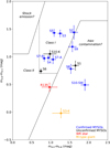 |
Fig. 3. MIR color-color diagram showing the Spitzer/IRAC colors of our confirmed MYSOs (blue dots) and the unconfirmed MYSO candidates (black dots). The Spitzer/IRAC photometric points of the MYSO candidates and S3-K are from Walborn et al. (2013). The photometric points of R135 are from the Spitzer/SAGE catalog (Meixner et al. 2006). Following the classification scheme of Gutermuth et al. (2009), we indicate the Class I and Class II regions and the regions where the Spitzer/IRAC colors might include unresolved knots of shock emission or resolved structured PAH emission. |
3. Reduction of VLT/X-shooter observations
We took spectra of our targets using the X-shooter spectrograph, which is mounted on the VLT (Vernet et al. 2011). X-shooter is an intermediate resolution (R ∼ 4000−17 000) slit spectrograph covering a wavelength range from 300 nm to 2500 nm divided over three arms: UV-Blue (UVB), visible (VIS), and near-infrared (NIR).
In Table 1 we present the log of our VLT/X-shooter observations. For the targets that have been previously resolved into multiple systems (i.e., S7, S8, S10, and S10-SW; Hyland et al. 1992; Rubio et al. 1992; Walborn et al. 2013), the X-shooter slit was positioned such that all targets would be observed within a single observation. Our spectra were taken in nodding mode, splitting the integration time of each observation into four nodding observations of each 670 s, 700 s, and 50 s for the UVB, VIS, and NIR arms, respectively. R135 was observed with only two nodding observations of 210 s, 240 s, and 50 s. Given their brightness, the observation in the VIS arm was split into two for S3-K and S5. The slit length was 11″ for each arm and the width was 1.0″, 0.9″, and 0.6″ for the UVB, VIS, and NIR arms, respectively. This results in a resolving power of 5100, 8800, and 8100, respectively. For the objects S1, S3-K, S4, S5, S6, S8, and R135, a slit width of 0.4″ was used in the NIR arm, which corresponds to a resolving power of 11 300. Unfortunately, the atmospheric dispersion corrector (ADC) was not working during our observations, which complicated the data reduction. The latter was especially an issue for the observations where we could not arrange the slit according to the parallactic angle, for instance, in the case multiple targets are included in one observation.
We reduced the data using the X-shooter Workflow for Physical Mode Date Reduction version 2.9.3. (Modigliani et al. 2010). The pipeline was implemented in the ESO-Reflex version 2.8 (Freudling et al. 2013). We performed a flux calibration using the spectrophotometric standard stars from the European Southern Observatory (ESO) database. The UVB and VIS fluxes were scaled to match the absolute fluxes in the NIR arm. We corrected our spectra for telluric features using the software tool MOLECFIT version 1.2.0 (Smette et al. 2015; Kausch et al. 2015).
3.1. Modeling the nebular emission
All our spectra were contaminated by strong nebular emission lines, see Fig. 4. Early type stars show mostly H and He lines in the X-shooter wavelength range that also have a nebular counterpart. Since these nebular counterparts are very strong, they first need to be removed before the spectral features that originate from the MYSO can be analyzed. Fortunately, the spectral resolution of X-shooter allows us to discriminate between the nebular emission and spectral features originating from the MYSOs (Kaper et al. 2011).
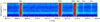 |
Fig. 4. Reduced 2D science frame of S4 as assessed from the pipeline. We show a single nodding position. The color indicates flux, where red and blue are high and low flux, respectively. The spatial position is with respect to the center of the slit. The figure is centered around the [S II] 671.6,673.1 nm lines (the two bright lines on the right) and the He I 667.8 nm line (the bright line on the left), all originating from the nebula. The three weak lines on the right are nebular Fe I lines. The continuum of S4 is visible in the lower part of the 2D frame. Additionally, some nebular continuum is visible. At the top, some weak continuum from an object not analyzed in this work. |
Our data were acquired in nodding mode; however, the nodding mode sky reduction results in an erroneous subtraction of the nebular emission as the nebular emission lines vary in strength and position (i.e., radial velocity (RV)) along the slit. We investigated these variations by reducing the nodding mode data in staring mode. The atmospheric contribution has not yet been subtracted at this stage.
To subtract the nebular lines, their variations along the X-shooter slit need to be modeled. We did this by extracting the spectrum from each spatial pixel along the slit and fitting the nebular lines. As line profile models, we used mainly a Gaussian distribution (GD), flat Gaussian distribution (FGD; Blázquez et al. 2008), and Moffat distribution (MD; Moffat 1969). The definitions of these functions can be found in Appendix A.1.
The 30 Dor region consists of multiple velocity components along each line of sight with a velocity dispersion of up to several tens of km s−1 (Torres-Flores et al. 2013; Mendes de Oliveira et al. 2017). If we identified multiple components in a nebular line, we used a combination of the models introduced above. For example, if the nebular line had two velocity components, we used two GDs to model these nebular lines. We assumed that the local continuum around a nebular line is roughly linear and therefore modeled it with a linear function. The lines were fit using a minimizing χ2 fitting routine.
As nebular lines are typically narrow, the range around the nebular line through which the continuum was fit was typically about ∼0.2 nm, ∼0.4 nm, and ∼0.7 nm for the UVB, VIS, and NIR arms, respectively. This corresponds to about ∼2, ∼5, and ∼4 velocity resolution elements, respectively, or to about ∼10, ∼20, and ∼12 data points per range. The number of wavelength bins per nebular line is thus relatively low, making it difficult to fit the lines. In addition to nebular lines, we fit the known [O I] 557.7 nm and O2 1280.3 nm sky emission lines to monitor possible sky variations along the slit. Sky variations were absent in all observations but for the usual variation at ≳2.25 μm. In Fig. 5 we show the modeled variation of the [S II] 671.6 nm nebular line along the spatial direction of the X-shooter slit (y-axis in Fig. 4). The line models for a few nebular lines can be found in Appendix A.2.
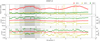 |
Fig. 5. Variations in the [S II] 671.6 nm nebular line along the slit, which is modeled with a triple Gaussian model. The variations are shown for one of the nodding mode positions of S4. Top: variations in the peak flux of each GD along the slit. Middle: variations in the central wavelength or RV shift of each GD along the slit. Bottom: variations in σ of each GD along the slit. In the dark, lighter, and lightest vertical gray zones, we show the 1σ, 2σ, and 3σ seeing ranges of the object, respectively. For more information, see the text. |
In modeling the nebular lines, we note that the measured variations in peak flux and position along the X-shooter slit differed between different ionization stages per element. We determined empirically that the different species may be subdivided into two main categories. We find that low ionization species (e.g., [O I], [O II], [N I], [N II], [S II], and [Ca II]) are in one category. The high ionization species (e.g., [O III], [S III], [Ar III], [Ne III], [Fe II], and [Ni II]) and nonforbidden transitions (e.g., He I, O I, Ba, Pa, and Br) are in the other category. This difference in variations along the X-shooter slit was taken into account when subtracting the nebular contamination.
3.2. Subtraction of nebular lines
The angular resolution of our observations is limited by the seeing. To accurately model the nebular emission in the spectra of our targets, the spatial extent of the target due to seeing has to be taken into account. We corrected for this by summing all spatial pixels within the angular resolution range of the target and fitting the nebular lines in the spectrum extracted from the range of spatial pixels. Typically, twice the angular resolution was used, but single angular resolution was used in crowded fields. Similarly, we fit the nebular lines for all ranges of spatial pixels outside of the object range, that is, all positions where we expect no flux of an MYSO to contribute to the nebular line flux.
We used a scaling method to subtract the nebular contamination from the MYSO candidate spectrum. In this method, we compute the nebular contribution in the object spectrum by scaling the nebular spectrum offset with respect to the object. The method goes as follows: we selected a region off-source to set as our “reference” nebular region, which was often a region relatively close to the object or a location where the nebular peak flux was approximately equally strong as the, at this point approximated, contribution on-source. At this off-source location, we set a reference line for each nebular line category, which was assumed to solely have a nebular, and thus no stellar, contribution. The forbidden lines are usually excellent candidates for this. However, if these could not be used, we used He I, Ba, or Pa lines for scaling. The latter was often necessary for the subtraction in the NIR arm as no strong forbidden lines are present in this wavelength range. The default scaling forbidden lines were [O II] 372.9 nm and [N II] 658.3 nm for the first scaling category in the UVB and VIS arm, respectively. For the second scaling category, we used the [Ne III] 386.9 nm and [S III] 631.0 nm in the UVB and VIS arm, respectively. In the NIR arm we generally only saw one category for which we used the Pa 1281.8 nm line. We note that forbidden lines may also originate from, for example, jets of the MYSO candidates. However, these jet lines are typically shifted (in RV) with respect to the nebular lines (Ellerbroek et al. 2011, 2013a; McLeod et al. 2018).
We determined the nebular contamination on-source by computing the scaling of the model parameters of the reference nebular line between the on-source spectrum and off-source spectrum, for example, Nsca = Non/Noff for the peak flux N. Next, we applied these scaling parameters to the off-source nebular line models, resulting in a model of the nebular lines in the on-source spectrum. We subtracted the nebular emission simply by subtracting the scaled nebular model from the on-source data, yielding the object spectrum with solely a sky contribution left.
The sky contribution was estimated by also subtracting the nebular contamination at an off-source location. This location was not necessarily the same position as the reference nebula. The local nebular contamination was subtracted without any scaling since we assume that no other emission sources are present at these distances from the object. This resulted in the sky continuum and emission lines at that spatial position. Some additional nebular continuum was present in the atmospheric spectra. However, if we assume that this is approximately constant along the spatial direction, this nebular continuum contribution was also present in the object spectrum. Assuming the atmospheric continuum and emission to be constant along the slit as well, the sky was subtracted of the object using this atmospheric spectrum. This yielded the object spectra free of nebular and atmospheric contamination but for some subtraction residuals.
The procedure described above was carried out at all nodding mode positions separately. The final nebular corrected spectra were then combined into a final object spectrum. We show the nebular corrected spectrum for S2 centered around the Ca II IRT in Fig. 6. The Ca II IRT does not show a nebular counterpart and is therefore assumed to originate from the object. In Fig. 6 we also performed the sky subtraction and telluric correction.
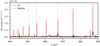 |
Fig. 6. Nebular and sky subtracted spectrum of S2 (black) and subtracted nebular contribution (red) centered around the Ca II IRT lines (indicated with vertical gray dashed lines). The nebular lines are Pa-11–19. Some residuals persist after the nebular subtraction. |
Residuals persist through the nebular subtraction process (see e.g., the right most Pa line in Fig. 6). Typically, these residuals were stronger for stronger nebular lines. Moreover, the nebular features were narrow and since nebular lines are significantly stronger than the continuum, a poor subtraction results in large residuals. Any residuals where therefore easily distinguishable from other spectral features.
4. Spectral analysis and target classification
A source is classified as a MYSO if it shows spectral emission features falling within two of the three following categories: (1) accretion features (Hα, β, Pa series, Ca II IRT, Brγ), (2) disk tracers (fluorescent Fe II 1697.8 nm, CO bandhead emission), and (3) outflowing material (H2 2121.8 nm, [Fe II] 1643.5 nm, [O I] 630.0 nm). Additionally, sources having three accretion features of which at least one has a red shoulder (indicative of inflowing material) are classified as MYSOs. Hα and Hβ were often saturated in the center due to the nebular contamination. Therefore, the centers of these lines had to be omitted in this analysis. The broad wings in these lines, however, are of stellar origin and used for the detection of potential inflow. Most of our targets do not show photospheric absorption lines hence these could not be used for classification purposes. When photospheric features were present, we determined the spectral type (SpT) using the classification scheme of Gray & Corbally (2009). In the following subsections we present the spectroscopic results for all objects. A summary of all detected spectral features for each object and the final classification is shown in Table 2. In Appendix B we show the investigated spectral regions for all targets.
Detected spectral features and target classification.
4.1. S1 and S1-SE
These objects are located relatively far away from 30 Dor’s central cluster R136, see Fig. 1. The region, also called the Skull Nebula, is associated with the larger CO cloud 30 Dor-06 of Johansson et al. (1998) and H II region No. 889 of Kastner et al. (2008). It is located between an X-ray cavity that is possibly associated with three nearby WR stars (R144, R146, and R147; Townsley et al. 2006) and the older Hodge 301 cluster known to have hosted multiple supernovae (Grebel & Chu 2000; Cignoni et al. 2016).
S1 is resolved into multiple objects with I-band (900 nm) magnitudes of ∼19−21 (Walborn et al. 2013). In our observation, we did not resolve multiple components. We, therefore, do not probe this multiplicity and consider S1 as a single source. We observe weak continuum in the UVB arm, which gets stronger toward the VIS and NIR arms. We detect very weak Ba and Pa absorption lines, the Pa jump, and [O I] 630.0 nm emission. We cannot confirm a MYSO nature.
Walborn et al. (2013) suggest S1-SE to have two components; we, however, cannot confirm this. S1-SE is fainter than S1 and shows no detectable continuum up to about 800 nm. The signal-to-noise ratio (S/N) is insufficient in detecting any spectral features, except for some weak H2 2121.8 nm emission.
4.2. S2
S2 is a relatively faint source located southwest to R136 in the head of a dust pillar and appears multiple in NICMOS data (Walborn et al. 1999). We do not resolve the object in our observation. Assuming a single (or compact multiple) origin, Walborn et al. (2013) estimated a luminosity L = 3.4 × 10⁴ L⊙, effective temperature Teff = 12 000 K, stellar mass M = 20.1 M⊙, and extinction AV = 6.5 mag.
It is a very red source with relatively modest NIR excess. We only detect continuum from about ∼1500 nm onward, increasing with wavelength. The Ba and Pa series are not detected except for broad Hα emission with a red shoulder. Though this is an indication of a possible inflow, it could also be produced by the companion. The [O I] 630.0 nm emission is contaminated by nebular subtraction residuals. S2 does show strong single-peaked Ca II IRT emission (see e.g., Fig. 6) together with weak Brγ emission. We classify S2 as a MYSO.
4.3. S3, S3-K, and R135
The complex of S3, S3-K, and the isolated WR star R135 lies to the northwest of R136 within a dust filament. Walborn et al. (2013) observe that at wavelengths shorter than the Ks-band S3-K dominates over S3; whereas at longer wavelengths of 4.5 μm and 8.0 μm, S3 dominates the entire region. Additionally, they determined L = 8.2 × 10⁴ L⊙, Teff = 38 000 K, M = 25.2 M⊙, and AV = 10.0 mag for S3 and suggest S3-K to be a star with T = 4750 K and AV = 5.85 mag rather than a YSO by finding a better fit with photospheric models than with YSO models.
Our spectrum of S3 has a relatively low S/N and is dominated by nebular subtraction residuals hampering the identification of intrinsic spectral features. The continuum becomes visible around ∼1600 nm and shows only a moderate increase in strength toward longer wavelengths. A broad emission feature is present around Hα and we detect Fe II 1687.8 nm and H2 2121.8 nm emission. The Pa series is completely dominated by nebular subtraction residuals; only Paβ shows some weak emission. Similarly, Brγ, and [O I] 630.0 nm show emission features that are contaminated by residuals of the nebular subtraction. According to Walborn et al. (2013), S3 is the second most massive MYSO candidate of our sample. Here, we confirm the MYSO nature of S3.
In our observation, S3-K becomes visible from about 400 nm onward and is very bright in the Ks-band. The Ba series are not visible but for some subtraction residuals. The Pa series is weakly in absorption and [O I] 630.0 nm is absent. The spectrum is dominated by CO, TiO, and other molecular absorption bands as well as various narrow absorption lines. Additionally, we see that the Ca II IRT exhibits absorption. The SpT should be early M or possibly late K due to the presence of many molecular bands and Ca II, Fe I, and Ti I absorption features. The effective temperature of Walborn et al. (2013) indicates SpT ∼ K3. S3-K is, however, too bright to be a typical M- or K-type MS star at the distance of 30 Dor. Fitting the Ca II IRT yields a RV of 261.4 ± 0.8 km s−1, which is consistent with the surrounding region (Torres-Flores et al. 2013). This excludes the suggestion of S3-K being a foreground star. S3-K may be explained as a ∼10 M⊙ M-type (super)giant, which is further supported by the fact that the flux does not strongly increase in the Spitzer/IRAC bands.
R135 is a WR star of SpT WN7h+OB (VFTS 402; Evans et al. 2011). In our X-shooter spectra, we are not able to detect spectral features of a possible OB-type companion due to dilution by the WR star. We identify broad emission in all hydrogen series (i.e., Ba, Pa, and Br) and strong N III emission features. Using the classification scheme of Smith (1968), we classify the WR star as a WN7h star. This is in agreement with the earlier classification of Evans et al. (2011).
4.4. S4
S4 is located in the head of a bright-rimmed pillar oriented toward R136 (Walborn et al. 1999, 2002). It is one of the most luminous sources in 30 Dor at almost all NIR wavelengths and has the strongest NIR excess of all the targets in our sample. Walborn et al. (2013) determined L = 10.7 × 10⁴ L⊙, Teff = 39 000 K, M = 27.4 M⊙, and AV = 1.8 mag. S4 has a companion (IRSW-26; Rubio et al. 1998) to the southwest, which is ≳3 mag fainter in the Ks-band. We, therefore, analyze S4 as a single object.
The continuum of S4 is visible across the entire X-shooter wavelength range, but it becomes substantially stronger from the J-band onward. The nebular contamination was very strong resulting in the saturation of multiple nebular lines, including Hα, β. Nevertheless we see clear signatures of in-falling material in the wings of these lines manifested by the red shoulders. In Fig. 7 we show the spectral features used for the classification. Furthermore, we detect several Fe II emission features and weak CO bandheads indicative of a disk and [Fe II] and H2 lines, which are indications of a bipolar outflow (Ellerbroek et al. 2013a). S4 is the most massive MYSO in Walborn et al. (2013), which is in agreement with the spectral features being the most prominent of all our targets. S4 is a MYSO.
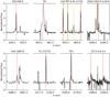 |
Fig. 7. [O I] 630.0 nm, Hα, Ca II IRT and Pa-13–16, [Fe II] 1643.5 nm, Fe II 1687.7 nm, H2 2121.8 nm, Brγ, and the 2–0 and 3–1 CO bandhead regions shown for S4. For clarity, the [Fe II] 1643.5 nm, Fe II 1687.7 nm, H2 2121.8 nm, Brγ, and CO bandhead regions have been enhanced by a factor of 5 and 15, respectively. We indicate the positions of the transitions by the red dashed lines. The Pa series and Br-8 line are marked by yellow dash-dotted lines for clarification. The center of Hα was saturated due to nebular emission and has been clipped. All narrow features are either telluric lines or residuals from the nebular or sky subtraction. |
4.5. S5
S5 is situated in a boomerang-shaped molecular cloud located north of R136 (Walborn et al. 1999; Kalari et al. 2018). The X-shooter slit includes six targets, which we labeled A–F, see Fig. 8.
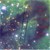 |
Fig. 8. HST/WFPC2/F814W (red) +F555W (green) +F336W (blue) composite image (20″ × 20″) of the cluster field surrounding S5 (Walborn et al. 2002). North is up and east is to the left. The two nodding positions of the X-shooter slit are shown with the two black rectangles. We identify a total of six continuum sources in our observation, which we labeled A–F (indicated in red). Even though S5-E is not visible in this image, we still indicate its presumed location. |
S5-A is the brightest of the six objects at optical wavelengths. Walborn et al. (2014) identified S5-A as a O((n)) star, whereas we classify S5-A as an O6 V((f)) star. The difference with Walborn et al. (2014) is due to the nebular contamination or larger residuals that are still present in their observations, whereas we subtracted that, allowing for a more precise spectral classification. We determined a RV of 246.2 ± 11.0 km s−1. This is in agreement with the RV observations of Sana et al. (2013).
S5-B and S5-C are less bright. They show strong Ba and He I absorption from which we determined a SpT of B0 V for both objects. The S/N was not optimal, hence this classification is rather uncertain. We find a RV of 254.6 ± 4.9 and 247.1 ± 10.9 km s−1 for S5-B and S5-C, respectively.
S5-D is an object which only shows significant brightness in the VIS arm of X-shooter. It shows Ca II IRT absorption lines. This suggests that S5-D is a late-type star. We determined a RV of 19.5 ± 3.0 km s−1, implying S5-D is a foreground star.
S5-F is located at the edge of the X-shooter slit and is only visible in the UVB and blue part of the VIS arms due to the ADCs malfunctioning. In the UVB arm, we detect rising intensity toward longer wavelengths accompanied with weak Ba and He I absorption features. Due to the low S/N, we cannot further constrain the SpT than early-B or late-O. We determined a RV of 221.0 ± 4.0 km s−1.
S5-E is the actual MYSO candidate selected to be observed. It has been identified as a MYSO candidate by Gruendl & Chu (2009) and later the young nature of S5-E was confirmed (Seale et al. 2009; Jones et al. 2017). According to Walborn et al. (2013), S5-E becomes apparent from the Ks-band onward. They estimate a lower limit of > 19 for the J-band magnitude. On the X-shooter slit, S5-E shows contamination from S5-A in the UVB and VIS arms. The continuum of S5-E appears around 1500 nm and is brighter than S5-A from about 2000 nm onward. Despite the contamination by S5-A, we can recognize weak Ca II IRT, H2 2121.8 nm, and CO first-overtone bandhead emission. This allows us to classify S5-E as a MYSO.
4.6. S6
S6 could represent a case of monolithic massive star formation due to its isolated position (Walborn et al. 2002). SED fitting of the NIR and MIR photometric points results in L = 3.7 × 10⁴ L⊙, Teff = 34 000 K, M = 18.4 M⊙, and AV = 3.0 mag (Walborn et al. 2013). S6 shows an NIR excess similar to S4. We detect continuum from about 800 nm onward, which gets substantially stronger beyond 1500 nm. Besides weak Pa emission features, no other spectral features are visible. Walborn et al. (2013) classify S6 as a Class I MYSO, where according to the classification scheme of Megeath et al. (2004), it should be a Class II object. Spectroscopically we cannot confirm S6 as a MYSO.
4.7. S7-A and S7-B
The complex of S7-A and S7-B is embedded in a large dust pillar oriented toward R136 (Walborn et al. 1999, 2002). In the Y-band, S7-A is brighter than S7-B; from the J-band onward, S7-B dominates over S7-A (Walborn et al. 2013). Both targets show strong NIR excess, with S7-B being the third brightest Ks-band target in our sample after S4 and S6, see Fig. 2. Both targets fit on one X-shooter slit. Unfortunately, the observations were taken under bad seeing conditions (average 2.2″).
By SED fitting of the NIR and MIR photometric points of S7-A, Walborn et al. (2013) determined L = 3.0 × 10⁴ L⊙, Teff = 30 000 K, M = 15.2 M⊙, and AV = 3.2 mag. Nayak et al. (2016) classify S7-A (J84.695932−69.083807 in their paper) as a Type II YSO with L = 5.62 × 10⁴ L⊙ and M = 21.8 M⊙. We detect continuum in the UVB arm, which gets weaker toward longer wavelengths. Eventually, it almost disappears around ∼1000 nm and reappears from about ∼1500 nm onward. Photospheric Ba and He I absorption features are detected and Hα shows broad emission. From the photospheric absorption features, we determined a RV of 264.7 ± 2.3 km s−1 and classify S7-A as a B1 V star. The Pa series shows weak emission features with nebular subtraction residuals superimposed. Additionally, we detect broad Brγ, Fe II 1687.8 nm, H2 2121.8 nm, and weak CO first-overtone bandhead emission. The detected spectral features confirm a MYSO nature.
S7-B is the brightest of the two objects in the NIR and MIR. Nayak et al. (2016) classify S7-B (J84.695173−69.084857 in their paper) as a Type II YSO with L = 5.62 × 10⁴ L⊙ and M = 19.0 M⊙. We detect continuum over the entire X-shooter wavelength range. Unfortunately, no photospheric absorption features, similar to those in S7-A, are detected. We do detect broad Hα, Pa series, Fe II 1687.8 nm, Brγ (with a red shoulder), and H2 2121.8 nm emission. More remarkable are the strong (inversed) Ba and Pa jumps and the Pa series showing a blueshifted emission component, see Fig. 9. The latter seems to be double-peaked at velocities of about −355 km s−1 and −265 km s−1. This implies a RV of about −615 km s−1 and −525 km s−1 in the local reference frame, assuming a RV of 260 km s−1 for S7-B. This emission may originate from a very high velocity outflow or may be an effect of binary interaction. Besides the Pa series, this high blueshifed emission seems only weakly visible in the [Fe II] 1643.5 nm line. We classify S7-B as a MYSO.
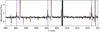 |
Fig. 9. Spectrum of S7-B centered around the three Pa lines. With the blue and red vertical dashed lines, we denote the locations of the blueshifted and redshifted peaks of emission at −355 km s−1 and −265 km s−1, respectively. The nebular counterpart of the Pa lines is indicated with the gray vertical lines at 250 km s−1. The region around ∼908 nm is a saturated [S III] nebular line. Other narrow features are either telluric features or residuals from the nebular subtraction. |
4.8. S8
S8 is a bright NIR source surrounded by a cluster of fainter objects (Walborn et al. 2002). In VMC observations, S8 is resolved into two objects of about equal magnitude, whereas in Spitzer observations, S8 is unresolved (Walborn et al. 2013). On the X-shooter slit, we were unable to resolve the two components despite the relatively good seeing conditions (average 0.8″) under which our observations were taken. Nayak et al. (2016) determined L = 5.62 × 10⁴ L⊙ and M = 19.0 M⊙ for S8 (J84.699755−69.069803 in their work) and classify it as a Type II YSO. We detect continuum from about 600 nm onward and observe broad Hα emission with a red shoulder. The Pa series shows emission contaminated by nebular subtraction residuals. Additionally, we see weak Ca II IRT and weak Brγ emission. We classify S8 as a MYSO.
4.9. S9
This red object is the brighter of two extended sources located in the vicinity of the optical multiple system within knot 2 of Walborn et al. (1999). This system includes VFTS 621; a young massive star of SpT O2 V((f*))z (Evans et al. 2011; Walborn et al. 2014). S9 is very bright in the Ks and Spitzer/IRAC 4.5 μm bands, but it is not dominant in the Spitzer/IRAC 8 μm band. S9 is a MYSO candidate according to Seale et al. (2009), and a water maser associated with S9 has been identified to the north (Ellingsen et al. 2010). Nayak et al. (2016) classify S9 (J84.703995−69.079110 in their work) as a Type I YSO and determined L = 6.81 × 10⁴ L⊙ and M = 23.9 M⊙ of S9. More recently, Reiter et al. (2019) computed L = 5.01 × 10⁵ L⊙, Teff = 21 120 K, and AV = 2.46 mag and see the CO bandheads in absorption, similar to S3-K in this work.
In our X-shooter observation, the continuum of S9 appears from about 1500 nm onward and increases only moderately in strength toward longer wavelengths. Some broad weak emission is present around Hα, H2 2121.8 nm, and Brγ; the Fe II 1687.8 nm feature is stronger. We do not detect any CO bandhead emission or absorption. S9 is a MYSO.
4.10. S10-A and S10-BC
In the Spitzer/IRAC wavelength bands, S10 appears as one of the brightest sources in 30 Dor. However, in the higher resolution VMC images, it actually splits up into three considerably fainter sources (Walborn et al. 2013). The system is located within a cavity created by VFTS 682; one of the most massive isolated WR stars (SpT WN5h, M ∼ 150 M⊙; Bestenlehner et al. 2011), which might be a runaway star from R136 (Renzo et al. 2019). The X-shooter slit was positioned such that all three objects would fit within a single exposure. However, we detect only two objects on the slit. While S10-A is resolved, S10-B and S10-C are not. The latter two are discussed under the name, S10-BC.
We detect the continuum of S10-A from about 1600 nm onward, which only increases moderately in strength toward longer wavelengths. We see emission features in the Pa series that are contaminated by some nebular subtraction residuals. No other spectral features are visible.
The continuum of S10-BC also becomes weakly visible from about 1600 nm onward and, similar to S10-A, increases moderately in strength toward longer wavelengths. We do not detect any features in the spectrum of S10-BC. Neither S10-A nor S10-BC can be confirmed to be a MYSO.
4.11. S10-K
S10-K is located to the southeast of the S10 region. Walborn et al. (2013) determined L = 0.7 × 10⁴ L⊙, Teff = 25 000 K, M = 9.1 M⊙, and AV = 4.4 mag. S10-K steeply raises in brightness from the J-band toward the Ks-band, but it does not notably increase further in flux in the Spitzer/IRAC bands. In our observation of S10-K, we start detecting continuum from about 1500 nm onward. Only weak Ca II IRT emission features and broad weak Hα emission are detected. We cannot confirm a MYSO nature.
4.12. S10-SW-A and S10-SW-B
This complex was labeled as S11 in Walborn et al. (2013) and is unresolved in their Spitzer images. The unresolved system was classified as a YSO candidate by Seale et al. (2009) and is located on the opposite side of the cavity created by VFTS 682 with respect to the S10 and S10-K region. A water maser has been identified at the location of S10-SW-A (Ellingsen et al. 2010). Nayak et al. (2016) determined L = 3.16 × 10⁴ L⊙ and M = 14.8 M⊙ for S10-SW-A (J84.720292−69.077084 in their paper) and they classify it as a Type I YSO.
The brightest component across all wavelengths is S10-SW-A for which we start detecting continuum from about 450 nm onward, which increases moderately in strength toward longer wavelengths. We see broad Hα and Hβ emission with a red shoulder. The Pa and Br series similarly show emission, but we are unable to detect a red shoulder. Due to the Pa emission, we are not able to detect possible Ca II IRT emission as these lines are superimposed on the Pa series. Additionally, we detect Fe II 1687.8 nm and H2 2121.8 nm emission. We classify S10-SW-A as a MYSO.
S10-SW-B becomes visible from about 1700 nm onward. Hα shows weak emission and displays a weak red shoulder. The [O I] 630.0 nm line, Ca II IRT, and H2 2121.8 nm show weak indications of emission. S10-SW-B is a MYSO.
4.13. Spectral energy distributions
In Figs. 10 and 11 we show the SEDs of all of our targets. We overplotted four Castelli & Kurucz models corresponding to the SpTs derived in the sections above (Kurucz 1993; Castelli & Kurucz 2004). For the targets with unknown SpT, we plotted the Castelli & Kurucz models of a B0 V star. All model fluxes are scaled to the 30 Dor distance by correcting with a factor (R⋆/d)2 for R⋆ = 15 R⊙ and d = 50 kpc. For S3-K, we use R⋆ = 100 R⊙, and for R135, we use the WN model SED of Bestenlehner et al. (2014). In most of our objects, a NIR excess is clearly visible in Figs. 10 and 11. Additionally, we can deduce from Figs. 10 and 11 that the extinction AV is between 5 and 10 mag for most targets.
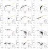 |
Fig. 10. SEDs of S1–S5-F. The spectrum of each object is shown in black and has been smoothed by a factor of 100. The confirmed MYSOs are indicated in bold. The objects S5-B, S5-C, S5-D, and S5-F were not corrected for slit loss since we lack photometry of these objects. The telluric absorption bands around 1.1 μm, 1.5 μm, and 2.0 μm are clipped. Additionally, we clipped the spectrum above 2.25 μm due to sky variations and at short wavelengths for S2, S3, and S5-E due to the low flux of these objects. Literature photometric points are shown as the yellow diamonds (Parker 1992; Cutri et al. 2003; Kato et al. 2007; Walborn et al. 2013; Gaia Collaboration 2016). Upper limits are indicated with an arrow. With the dashed lines, we plotted a Castelli & Kurucz model for various AV. |
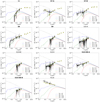 |
Fig. 11. Same as Fig. 10, but for the objects S6-R135, where we clipped S6, S9, S10-A, S10-BC, S10-K, and S10-SW-B at short wavelengths. |
5. Discussion
5.1. Near-infrared excess
All our MYSO candidates show a strong NIR excess, which suggests that our targets are surrounded by a disk or envelope. The excess is more than 5 mag for the brightest Ks-band targets. The NIR photometric points were adopted from Walborn et al. (2013), who used observations of the VMC and fit point spread functions to the objects. Not all the excess flux of our sources may, however, be associated with the MYSO candidates. Some surrounding nebular (dust) emission may have been included in their photometric computations, resulting in an overestimate of the brightness of the MYSO candidates. Our best angular resolution in terms of seeing is about 0.7″, which corresponds to ∼35 000 AU (∼0.2 pc) in the plane of the sky at the distance of 30 Dor. This means that many of our targets may be blended with surrounding stars. Moreover, since 70% of the Galactic massive stars reside in close binary or higher order multiples (Sana et al. 2012), many of our targets ought to be unresolved multiple systems.
We investigated the NIR excess with our X-shooter spectra. Our spectra were corrected for slit loss by multiplying our flux calibrated spectra, as acquired from the X-shooter pipeline, with a photometric correction factor in order to match them with the photometric observations of Walborn et al. (2013). However, with the flux calibrated spectra from the X-shooter pipeline, we can determine an upper limit to the photometric points (i.e., lower limit to the brightness) by not correcting for slit loss. To get an unbiased upper limit, we also did not correct for the malfunctioning ADCs in the UVB and VIS arms, that is, by not imposing that the edges of the X-shooter arms overlap.
We can determine the apparent magnitude mi in the photometric band i by numerically integrating the flux in the band,
 (1)
(1)
where ℱi, λ is the flux at wavelength λ, Si, λ is the filter curve, and ℱi, 0 is the flux zero point of the band. For the B, V, R, and I-bands, we used the Bessell photometric system (Bessell 1990). For the G-band, we used the Gaia photometric system (Gaia Collaboration 2016), and for the Y, J, H, and Ks-bands, we used the VISTA photometric system1. In the computation of the magnitudes, we clipped the regions surrounding the subtracted nebular lines so that any subtraction residuals would not contribute to the calculation. We also clipped the edges of the X-shooter arms because of the significant noise and low detector response in these regions and the part of the spectrum from 2250 nm onward due to a gradient along the slit of continuum produced in the Earth’s atmosphere having a significant impact on the measured fluxes.
We present the computed upper limits to the magnitudes for all our objects in Appendix C. In the left part of Fig. 12, we plotted a NIR color-magnitude diagram with our upper limits. The color-axis in Fig. 12 results from the subtraction of two upper limits and is therefore ambiguous. Nevertheless, we still observe a strong NIR excess for almost all our MYSO targets, though the strength of the excess is, on average, ∼2 mag less compared to Fig. 2. In the right part of Fig. 12, we plotted a VIS color-magnitude diagram of the upper limits. Using the VIS color-magnitude diagram, we can check the validity of Eq. (1). If the objects with optical flux would show an excess in the VIS color-magnitude diagram, Eq. (1) would fail to reproduce physical results for sure. All our objects, except for the WR star R135, are well below the O3 V reddening lines.
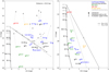 |
Fig. 12. Left: NIR color-magnitude diagram of the upper limits derived from our X-shooter spectra (see Appendix C). Error bars are omitted for clarity, but they may be found in Appendix C; the typical error is ∼0.6 mag. The gray lines link our upper limit with the literature values (gray dots and arrows). All of the other lines are the same as in Fig. 2. We note that the color is composed of a subtraction of two upper limits and, therefore, it is uncertain. Right: optical color-magnitude diagram of the upper limit photometric points. In the VIS range, the photometric upper limits are well below the reddening line. Again the color is composed of a subtraction of two upper limits and, therefore, it is uncertain. |
5.2. Confirmation of MYSOs
The confirmation of ten MYSOs with X-shooter data marks the first spectroscopic confirmation of most of these MYSOs. All our targets were selected based on the top ten Spitzer MYSO candidates as identified by Walborn et al. (2013). They determined the mass of their MYSO candidates by mostly using NIR and MIR photometric points and the YSO models of Robitaille et al. (2006). At these wavelengths, the radiation mostly emerges from the accretion disk and (inner) envelope; the stellar mass thus had to be estimated from disk and envelope properties. Since the relation between the disk, envelope, and star is not well established, the mass estimate is rather uncertain. They report S4 as the most massive MYSO (M = 27 M⊙). In our observations, S4 is the most prominent MYSO. Due to the lack of photospheric lines, we cannot provide a mass estimate of this source.
According to the classification scheme of Megeath et al. (2004), S6 should be a Class II object. Spectroscopically, we do not confirm S6, and the lack of any optical emission suggests that, if S6 is a MYSO, it is still deeply embedded. Nayak et al. (2016) classify S7-A as a Type II MYSO. We confirm S7-A as a MYSO and detect photospheric lines, which suggests that it might be a Class II object. S7-B is also a Type II MYSO in their work; however, the lack of photospheric lines in this work hints at a Class 0/I nature rather than a Class II nature. All other confirmed MYSOs, S2, S3, S4, S8, S9, S10-SW-A, and S10-SW-B, are Type I YSOs (Nayak et al. 2016). Furthermore, two MYSO candidates that were identified with Spitzer/IRS (i.e., S5-E and S10-SW-A) are confirmed here as MYSOs (Seale et al. 2009; Jones et al. 2017).
S9 was also a Spitzer/IRS MYSO candidate, and it was the most massive MYSO in the sample of Nayak et al. (2016), although they may have mixed S9 with the massive young star VFTS 621 since they refer to S9 as the object with SpT O2. More remarkably is the absence of the CO bandhead absorption observed by Reiter et al. (2019). Our observations were taken about three years earlier; however, variability on timescales of ∼1 yr have been observed for, for example, FU Orionis type stars (Contreras Peña et al. 2017).
We can determine whether our confirmed MYSOs are indeed massive by deriving their luminosity and using a mass-luminosity relation to estimate the mass. For this, we used the J-band since the disk does not completely dominate over the central star there yet and also because the extinction in this band is rather low. We computed the luminosity both for the magnitudes reported by Walborn et al. (2013) and for the magnitude upper limits presented in this work (see Appendix C). In the latter case, the resulting luminosity and mass is a lower limit. The results of the calculation are show in Table 3, where we used AV = 5 and the bolometric correction (BCJ) following Martins & Plez (2006) for the corresponding SpT (B0 V was used for the targets with an unknown SpT). Typically, our luminosity lower limits are about 0.5 dex lower than the luminosities derived from the photometric points of Walborn et al. (2013). The mass was estimated using a typical ZAMS L−M relation (L ∝ M3.5). We did not compute errors on the mass lower limits since our estimates are based on proportionality. Except for S2, all confirmed MYSOs show luminosities and masses that are consistent with a massive star nature. We note that S2 may still be a massive star because the mass estimate is a lower limit and based on the assumption of the source already being on the ZAMS.
Lower limit luminosities and masses computed from X-shooter upper limits to the magnitudes.
5.3. Comparison to other samples
Strong emission lines, such as the Ca II IRT and Brγ, are indicative of inflow of circumstellar material. We detect Ca II IRT emission toward 50% of the confirmed MYSOs, which is in agreement with the Galactic star forming region M17 (66%; Ramírez-Tannus et al. 2017). Our detection rate of Brγ is 80%, which is consistent with the high detection rate in other LMC samples (Ward et al. 2016; Ward 2017; Reiter et al. 2019), SMC samples (Ward et al. 2017; Reiter et al. 2019), and larger Galactic samples (Cooper et al. 2013; Pomohaci et al. 2017). In Fig. 13 we show the Brγ luminosity of our confirmed MYSOs against the absolute K-band magnitude. For our sources, the Ks-band magnitudes of Walborn et al. (2013) and AV = 5 were adopted; for the LMC MYSOs of Reiter et al. (2019), we find lower luminosities with their Brγ fluxes. The main difference between Galactic and Magellanic MYSOs is the difference in metallicity. Ward et al. (2017) suggest that the Brγ luminosity, which is a probe of the accretion luminosity, increases with decreasing metallicity. However, the spread of the data points of the Magellanic Clouds in Fig. 13 is too large to see any significant correlation.
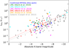 |
Fig. 13. Luminosity of Brγ plotted against the absolute K-band magnitude. Various MYSO samples in the LMC, SMC, and our Galaxy are overplotted. With the gray and red lines, we indicate the empirically derived relations of Cooper et al. (2013) and Ward et al. (2017) for our Galaxy and the SMC, respectively. |
Another metallicity dependent observable might be the detection rate of fluorescent Fe II and CO bandheads. Both of these are tracers of an accretion disk. In total, 70% of our confirmed MYSOs show either fluorescent Fe II or CO bandhead emission, which is higher than the Galactic rate of ∼40% (Cooper et al. 2013; Ellerbroek et al. 2013a; Ramírez-Tannus et al. 2017; Pomohaci et al. 2017). However, we have a small sample and are biased toward brighter targets. Adding the LMC samples of Ward et al. (2016, only CO bandheads), Ward (2017), and Reiter et al. (2019) gives a combined detection rate of 47% for either Fe II or CO bandheads, or both. This is consistent with the Galactic rate, yet the combined LMC sample is still significantly smaller.
5.4. Outflows
Outflows are thought to be common in MYSOs (e.g., Zhang et al. 2001, 2005). They can be characterized by [O I] 630.0 nm, H2, or [Fe II] showing emission, occasionally with an offset RV of up to a few hundred km s−1 (Ellerbroek et al. 2013a). Of our confirmed MYSOs, 80% show outflow signatures. [O I] 630.0 nm emission is detected for 40% of the MYSOs; however, the identification was often hampered by residuals of the nebular subtraction. S2 and S8 are the only confirmed MYSOs that do not show any H2 2121.8 nm emission. The RV of H2 2121.8 nm in all sources shows no significant offset from the assumed systemic velocity (250−260 km s−1). [Fe II] 1643.5 nm is only detected toward S4 and S7-B. While the RV of [Fe II] 1643.5 nm in S4 is around the systemic velocity, S7-B shows double-peaked [Fe II] 1643.5 nm and Pa series emission with a RV of −615 km s−1 and −525 km s−1 in the local frame of reference. The two velocities might indicate so-called bullets in the outflow, that is, enhancements in density and temperature at certain positions compared to the rest of the outflow.
Another measure of bipolar outflow is the presence of H2O maser emission. Water masers coinciding with the locations of S9 and S10-SW-A have been reported by Ellingsen et al. (2010). This is consistent with the detection of H2 2121.8 nm for these sources in this work.
6. Summary
We present the results on a spectroscopic analysis of the top ten Spitzer MYSO candidates in 30 Dor of Walborn et al. (2013). These targets are resolved in ∼20 sources. We took advantage of the unparalleled spectral resolution (R ∼ 4000−17 000) and wavelength coverage (300−2500 nm) of VLT/X-shooter to detect spectral features that are characteristic of MYSOs.
All VLT/X-shooter spectra of the MYSO candidates were contaminated by nebular emission. We used a scaling method developed in this work to subtract this nebular contamination from our spectra, revealing the spectral features intrinsic to the MYSOs.
Photometric observations from the literature suggest that our objects possess a strong NIR excess, indicating the presence of an accretion disk. We computed photometric upper limits using our X-shooter spectra. These limits still indicate the presence of a strong NIR excess. This indicates that our targets are surrounded by a large amount of circumstellar dust.
We spectroscopically confirm S2, S3, S4, S5-E, S7-A, S7-B, S8, S9, S10-SW-A, and S10-SW-B to be MYSOs by the detection of features, such as the Ca II, Brγ, fluorescent Fe II, H2, and CO first-overtone bandhead emission. We computed luminosity and mass lower limits for our targets, which support a massive star nature for all confirmed MYSOs, except S2. S7-A shows photospheric lines, which hint at a Class II MYSO origin. All other confirmed MYSOs seem to have a Class 0/I origin.
We computed the Brγ luminosity for all confirmed MYSOs and find that these are consistent with other samples in the LMC and SMC (Ward et al. 2016, 2017; Ward 2017; Rubio et al. 2018; Reiter et al. 2019). Due to the large scatter in data points, no clear correlation was seen between the Brγ luminosity (i.e., accretion luminosity) and metallicity. Combining our detection rate of disk tracers, such as fluorescent Fe II and CO bandhead, with those of other LMC samples of Ward et al. (2016) and Reiter et al. (2019) is consistent with the Galactic rate (∼40%; Cooper et al. 2013)
We detect signatures of an outflow in 80% of MYSOs through the detection of [O I] 630 nm, H2 2121.8 nm, and [Fe II] 1643.5 nm. S7-B might show so-called bullets (i.e., enhancements in density and temperature) in the outflow. Future analysis of this outflow is required to confirm its nature and composition.
With this still rather small sample of MYSOs, we studied massive star formation in the most extreme massive star forming region in the Local Group. Modeling the emission and NIR excess of disk models can provide insight into how these massive stars form and evolve. In particular, the effect of metallicity on the accretion luminosity can be studied by comparing these models to their Galactic counterparts. This sample contains several MYSOs that are still deeply embedded in their birth clouds. With current submillimeter telescopes, such as the Large Millimeter/submillimeter Array (ALMA), we can study the gaseous molecular content of these MYSOs (e.g., CO; Nayak et al. 2016). The angular resolution of ALMA is, however, still insufficient to spatially resolve these MYSOs. Future optical, NIR, and MIR facilities, such as the James Webb Space Telescope and Extremely Large Telescope, will be vital in further characterizing the still poorly understood process of formation of massive stars, both in our Galaxy and in the Magellanic Clouds.
Acknowledgments
We would like to thank the anonymous referee for his/her useful comments on the manuscript. Based on observations collected at the European Southern Observatory under ESO program 088.D-0850(A) and 090.C-0346(A). We thank the ESO support staff (including former DG Tim de Zeeuw) for carrying out the observations. LK and JJ acknowledge support from NOVA and an NWO-FAPESP grant for advanced instrumentation in astronomy. The work of M.S. is based upon work supported by NASA under award number 80GSFC17M0002. This work made use of observations made with the NASA/ESA Hubble Space Telescope, and were obtained from the Hubble Legacy Archive, which is a collaboration between the Space Telescope Science Institute (STScI/NASA), the Space Telescope European Coordinating Facility (ST-ECF/ESA) and the Canadian Astronomy Data Centre (CADC/NRC/CSA).
References
- Alcalá, J. M., Natta, A., Manara, C. F., et al. 2014, A&A, 561, A2 [NASA ADS] [CrossRef] [EDP Sciences] [Google Scholar]
- Andre, P., Ward-Thompson, D., & Barsony, M. 2000, in Protostars and Planets IV, eds. V. Mannings, A. P. Boss, & S. S. Russell, 59 [Google Scholar]
- Bachiller, R. 1996, ARA&A, 34, 111 [NASA ADS] [CrossRef] [Google Scholar]
- Beltrán, M. T., & de Wit, W. J. 2016, A&ARv, 24, 6 [NASA ADS] [CrossRef] [Google Scholar]
- Bessell, M. S. 1990, PASP, 102, 1181 [NASA ADS] [CrossRef] [Google Scholar]
- Bestenlehner, J. M., Vink, J. S., Gräfener, G., et al. 2011, A&A, 530, L14 [NASA ADS] [CrossRef] [EDP Sciences] [Google Scholar]
- Bestenlehner, J. M., Gräfener, G., Vink, J. S., et al. 2014, A&A, 570, A38 [NASA ADS] [CrossRef] [EDP Sciences] [Google Scholar]
- Beuther, H., Churchwell, E. B., McKee, C. F., & Tan, J. C. 2007, Protostars and Planets V (Tucson: University of Arizona Press), 165 [Google Scholar]
- Bik, A., & Thi, W. F. 2004, A&A, 427, L13 [NASA ADS] [CrossRef] [EDP Sciences] [Google Scholar]
- Bik, A., Kaper, L., & Waters, L. B. F. M. 2006, A&A, 455, 561 [NASA ADS] [CrossRef] [EDP Sciences] [Google Scholar]
- Blázquez, J., García-Berrocal, A., Montalvo, C., & Balbás, M. 2008, Metrologia, 45, 503 [NASA ADS] [CrossRef] [Google Scholar]
- Blum, R. D., Barbosa, C. L., Damineli, A., Conti, P. S., & Ridgway, S. 2004, ApJ, 617, 1167 [NASA ADS] [CrossRef] [Google Scholar]
- Brandner, W., Grebel, E. K., Barbá, R. H., Walborn, N. R., & Moneti, A. 2001, AJ, 122, 858 [NASA ADS] [CrossRef] [Google Scholar]
- Castelli, F., & Kurucz, R. L. 2004, in New Grids of ATLAS9 Model Atmospheres, eds. N. Piskunov, W. W. Weiss, & D. F. Gray, A20 [Google Scholar]
- Chen, C. H. R., Chu, Y.-H., Gruendl, R. A., Gordon, K. D., & Heitsch, F. 2009, ApJ, 695, 511 [NASA ADS] [CrossRef] [Google Scholar]
- Choi, J., Dotter, A., Conroy, C., et al. 2016, ApJ, 823, 102 [NASA ADS] [CrossRef] [Google Scholar]
- Churchwell, E. 2002, ARA&A, 40, 27 [Google Scholar]
- Cignoni, M., Sabbi, E., van der Marel, R. P., et al. 2015, ApJ, 811, 76 [NASA ADS] [CrossRef] [Google Scholar]
- Cignoni, M., Sabbi, E., van der Marel, R. P., et al. 2016, ApJ, 833, 154 [NASA ADS] [CrossRef] [Google Scholar]
- Cioni, M. R. L., Clementini, G., Girardi, L., et al. 2011, A&A, 527, A116 [NASA ADS] [CrossRef] [EDP Sciences] [Google Scholar]
- Contreras Peña, C., Lucas, P. W., Kurtev, R., et al. 2017, MNRAS, 465, 3039 [NASA ADS] [CrossRef] [Google Scholar]
- Cooper, H. D. B., Lumsden, S. L., Oudmaijer, R. D., et al. 2013, MNRAS, 430, 1125 [NASA ADS] [CrossRef] [Google Scholar]
- Crowther, P. A., Schnurr, O., Hirschi, R., et al. 2010, MNRAS, 408, 731 [NASA ADS] [CrossRef] [Google Scholar]
- Crowther, P. A., Caballero-Nieves, S. M., Bostroem, K. A., et al. 2016, MNRAS, 458, 624 [NASA ADS] [CrossRef] [Google Scholar]
- Cutri, R. M., Skrutskie, M. F., van Dyk, S., et al. 2003, VizieR Online Data Catalog: II/246 [Google Scholar]
- Dalton, G. B., Caldwell, M., Ward, A. K., et al. 2006, in The VISTA Infrared Camera, eds. I. S. McLean, & M. Iye, SPIE Conf. Ser., 6269, 62690X [Google Scholar]
- de Koter, A., Heap, S. R., & Hubeny, I. 1997, ApJ, 477, 792 [Google Scholar]
- De Marchi, G., Panagia, N., Sabbi, E., et al. 2016, MNRAS, 455, 4373 [NASA ADS] [CrossRef] [Google Scholar]
- Dotter, A. 2016, ApJS, 222, 8 [NASA ADS] [CrossRef] [Google Scholar]
- Ellerbroek, L. E., Kaper, L., Bik, A., et al. 2011, ApJ, 732, L9 [NASA ADS] [CrossRef] [Google Scholar]
- Ellerbroek, L. E., Podio, L., Kaper, L., et al. 2013a, A&A, 551, A5 [NASA ADS] [CrossRef] [EDP Sciences] [Google Scholar]
- Ellerbroek, L. E., Bik, A., Kaper, L., et al. 2013b, A&A, 558, A102 [NASA ADS] [CrossRef] [EDP Sciences] [Google Scholar]
- Ellingsen, S. P., Breen, S. L., Caswell, J. L., Quinn, L. J., & Fuller, G. A. 2010, MNRAS, 404, 779 [NASA ADS] [CrossRef] [Google Scholar]
- Evans, C. J., Taylor, W. D., Hénault-Brunet, V., et al. 2011, A&A, 530, A108 [NASA ADS] [CrossRef] [EDP Sciences] [Google Scholar]
- Finkenzeller, U. 1985, A&A, 151, 340 [NASA ADS] [Google Scholar]
- Freudling, W., Romaniello, M., Bramich, D. M., et al. 2013, A&A, 559, A96 [NASA ADS] [CrossRef] [EDP Sciences] [Google Scholar]
- Gaia Collaboration (Prusti, T., et al.) 2016, A&A, 595, A1 [NASA ADS] [CrossRef] [EDP Sciences] [Google Scholar]
- Gray, R. O., & Corbally, J. C. 2009, Stellar Spectral Classification (Princeton, NJ: Princeton University Press) [Google Scholar]
- Grebel, E. K., & Chu, Y.-H. 2000, AJ, 119, 787 [NASA ADS] [CrossRef] [Google Scholar]
- Gruendl, R. A., & Chu, Y.-H. 2009, ApJS, 184, 172 [Google Scholar]
- Gutermuth, R. A., Megeath, S. T., Myers, P. C., et al. 2009, ApJS, 184, 18 [NASA ADS] [CrossRef] [Google Scholar]
- Hyland, A. R., Straw, S., Jones, T. J., & Gatley, I. 1992, MNRAS, 257, 391 [NASA ADS] [Google Scholar]
- Ilee, J. D., Wheelwright, H. E., Oudmaijer, R. D., et al. 2013, MNRAS, 429, 2960 [NASA ADS] [CrossRef] [Google Scholar]
- Ilee, J. D., Cyganowski, C. J., Nazari, P., et al. 2016, MNRAS, 462, 4386 [NASA ADS] [CrossRef] [Google Scholar]
- Ilee, J. D., Cyganowski, C. J., Brogan, C. L., et al. 2018a, ApJ, 869, L24 [NASA ADS] [CrossRef] [Google Scholar]
- Ilee, J. D., Oudmaijer, R. D., Wheelwright, H. E., & Pomohaci, R. 2018b, MNRAS, 477, 3360 [NASA ADS] [CrossRef] [Google Scholar]
- Johansson, L. E. B., Greve, A., Booth, R. S., et al. 1998, A&A, 331, 857 [NASA ADS] [Google Scholar]
- Jones, O. C., Woods, P. M., Kemper, F., et al. 2017, MNRAS, 470, 3250 [NASA ADS] [CrossRef] [Google Scholar]
- Kalari, V. M., Rubio, M., Elmegreen, B. G., et al. 2018, ApJ, 852, 71 [NASA ADS] [CrossRef] [Google Scholar]
- Kaper, L., Ellerbroek, L. E., Ochsendorf, B. B., & Caballero Pouroutidou, R. N. 2011, Astron. Nachr., 332, 232 [NASA ADS] [CrossRef] [Google Scholar]
- Kastner, J. H., Thorndike, S. L., Romanczyk, P. A., et al. 2008, AJ, 136, 1221 [NASA ADS] [CrossRef] [Google Scholar]
- Kato, D., Nagashima, C., Nagayama, T., et al. 2007, PASJ, 59, 615 [NASA ADS] [Google Scholar]
- Kausch, W., Noll, S., Smette, A., et al. 2015, A&A, 576, A78 [NASA ADS] [CrossRef] [EDP Sciences] [Google Scholar]
- Krumholz, M. R., Klein, R. I., McKee, C. F., Offner, S. S. R., & Cunningham, A. J. 2009, Science, 323, 754 [NASA ADS] [CrossRef] [PubMed] [Google Scholar]
- Kuiper, R., & Hosokawa, T. 2018, A&A, 616, A101 [NASA ADS] [CrossRef] [EDP Sciences] [Google Scholar]
- Kuiper, R., Klahr, H., Beuther, H., & Henning, T. 2011, ApJ, 732, 20 [NASA ADS] [CrossRef] [Google Scholar]
- Kurucz, R. L. 1993, VizieR Online Data Catalog: VI/039 [Google Scholar]
- Maíz Apellániz, J., Evans, C. J., Barbá, R. H., et al. 2014, A&A, 564, A63 [NASA ADS] [CrossRef] [EDP Sciences] [Google Scholar]
- Martins, F., & Plez, B. 2006, A&A, 457, 637 [NASA ADS] [CrossRef] [EDP Sciences] [Google Scholar]
- McLeod, A. F., Reiter, M., Kuiper, R., Klaassen, P. D., & Evans, C. J. 2018, Nature, 554, 334 [NASA ADS] [CrossRef] [Google Scholar]
- Megeath, S. T., Allen, L. E., Gutermuth, R. A., et al. 2004, ApJS, 154, 367 [NASA ADS] [CrossRef] [Google Scholar]
- Meixner, M., Gordon, K. D., Indebetouw, R., et al. 2006, AJ, 132, 2268 [NASA ADS] [CrossRef] [Google Scholar]
- Mendes de Oliveira, C., Amram, P., Quint, B. C., et al. 2017, MNRAS, 469, 3424 [NASA ADS] [CrossRef] [Google Scholar]
- Modigliani, A., Goldoni, P., Royer, F., et al. 2010, in Observatory Operations: Strategies, Processes, and Systems III, Proc. SPIE, 7737, 773728 [Google Scholar]
- Moffat, A. F. J. 1969, A&A, 3, 455 [NASA ADS] [Google Scholar]
- Nayak, O., Meixner, M., Indebetouw, R., et al. 2016, ApJ, 831, 32 [NASA ADS] [CrossRef] [Google Scholar]
- Oliveira, J. M., van Loon, J. T., Chen, C. H. R., et al. 2009, ApJ, 707, 1269 [NASA ADS] [CrossRef] [Google Scholar]
- Oliveira, J. M., van Loon, J. T., Sloan, G. C., et al. 2013, MNRAS, 428, 3001 [NASA ADS] [CrossRef] [Google Scholar]
- Parker, J. W. 1992, PASP, 104, 1107 [NASA ADS] [CrossRef] [Google Scholar]
- Paxton, B., Bildsten, L., Dotter, A., et al. 2011, ApJS, 192, 3 [Google Scholar]
- Paxton, B., Cantiello, M., Arras, P., et al. 2013, ApJS, 208, 4 [NASA ADS] [CrossRef] [Google Scholar]
- Paxton, B., Marchant, P., Schwab, J., et al. 2015, ApJS, 220, 15 [Google Scholar]
- Peimbert, M., Peimbert, A., & Ruiz, M. T. 2000, ApJ, 541, 688 [NASA ADS] [CrossRef] [Google Scholar]
- Pietrzyński, G., Graczyk, D., Gieren, W., et al. 2013, Nature, 495, 76 [NASA ADS] [CrossRef] [PubMed] [Google Scholar]
- Pomohaci, R., Oudmaijer, R. D., Lumsden, S. L., Hoare, M. G., & Mendigutía, I. 2017, MNRAS, 472, 3624 [NASA ADS] [CrossRef] [Google Scholar]
- Ramírez-Tannus, M. C., Kaper, L., de Koter, A., et al. 2017, A&A, 604, A78 [NASA ADS] [CrossRef] [EDP Sciences] [Google Scholar]
- Ramírez-Tannus, M. C., Cox, N. L. J., Kaper, L., & de Koter, A. 2018, A&A, 620, A52 [NASA ADS] [CrossRef] [EDP Sciences] [Google Scholar]
- Reiter, M., Nayak, O., Meixner, M., & Jones, O. 2019, MNRAS, 483, 5211 [NASA ADS] [CrossRef] [Google Scholar]
- Renzo, M., de Mink, S. E., Lennon, D. J., et al. 2019, MNRAS, 482, L102 [NASA ADS] [CrossRef] [Google Scholar]
- Robitaille, T. P., Whitney, B. A., Indebetouw, R., Wood, K., & Denzmore, P. 2006, ApJS, 167, 256 [NASA ADS] [CrossRef] [Google Scholar]
- Rolleston, W. R. J., Trundle, C., & Dufton, P. L. 2002, A&A, 396, 53 [NASA ADS] [CrossRef] [EDP Sciences] [Google Scholar]
- Rubio, M., Roth, M., & Garcia, J. 1992, A&A, 261, L29 [NASA ADS] [Google Scholar]
- Rubio, M., Barbá, R. H., Walborn, N. R., et al. 1998, AJ, 116, 1708 [NASA ADS] [CrossRef] [Google Scholar]
- Rubio, M., Barbá, R. H., & Kalari, V. M. 2018, A&A, 615, A121 [NASA ADS] [CrossRef] [EDP Sciences] [Google Scholar]
- Ruffle, P. M. E., Kemper, F., Jones, O. C., et al. 2015, MNRAS, 451, 3504 [NASA ADS] [CrossRef] [Google Scholar]
- Sabbi, E., Anderson, J., Lennon, D. J., et al. 2013, AJ, 146, 53 [NASA ADS] [CrossRef] [Google Scholar]
- Sabbi, E., Lennon, D. J., Anderson, J., et al. 2016, ApJS, 222, 11 [NASA ADS] [CrossRef] [Google Scholar]
- Salpeter, E. E. 1955, ApJ, 121, 161 [Google Scholar]
- Sana, H., de Mink, S. E., de Koter, A., et al. 2012, Science, 337, 444 [Google Scholar]
- Sana, H., de Koter, A., de Mink, S. E., et al. 2013, A&A, 550, A107 [NASA ADS] [CrossRef] [EDP Sciences] [Google Scholar]
- Schneider, F. R. N., Sana, H., Evans, C. J., et al. 2018a, Science, 359, 69 [NASA ADS] [CrossRef] [Google Scholar]
- Schneider, F. R. N., Ramírez-Agudelo, O. H., Tramper, F., et al. 2018b, A&A, 618, A73 [NASA ADS] [CrossRef] [EDP Sciences] [Google Scholar]
- Seale, J. P., Looney, L. W., Chu, Y.-H., et al. 2009, ApJ, 699, 150 [NASA ADS] [CrossRef] [Google Scholar]
- Seale, J. P., Looney, L. W., Chen, C. H. R., Chu, Y.-H., & Gruendl, R. A. 2011, ApJ, 727, 36 [NASA ADS] [CrossRef] [Google Scholar]
- Selman, F. J., & Melnick, J. 2013, A&A, 552, A94 [NASA ADS] [CrossRef] [EDP Sciences] [Google Scholar]
- Shimonishi, T., Onaka, T., Kato, D., et al. 2008, ApJ, 686, L99 [NASA ADS] [CrossRef] [Google Scholar]
- Shimonishi, T., Onaka, T., Kato, D., et al. 2010, A&A, 514, A12 [NASA ADS] [CrossRef] [EDP Sciences] [Google Scholar]
- Smette, A., Sana, H., Noll, S., et al. 2015, A&A, 576, A77 [NASA ADS] [CrossRef] [EDP Sciences] [Google Scholar]
- Smith, L. F. 1968, MNRAS, 138, 109 [NASA ADS] [CrossRef] [Google Scholar]
- Tan, J. C., Beltrán, M. T., Caselli, P., et al. 2014, Protostars and Planets VI (Tucson: University of Arizona Press), 149 [Google Scholar]
- Torres-Flores, S., Barbá, R., Maíz Apellániz, J., et al. 2013, A&A, 555, A60 [NASA ADS] [CrossRef] [EDP Sciences] [Google Scholar]
- Townsley, L. K., Broos, P. S., Feigelson, E. D., et al. 2006, AJ, 131, 2140 [NASA ADS] [CrossRef] [Google Scholar]
- van der Plas, G., van den Ancker, M. E., Fedele, D., et al. 2008, A&A, 485, 487 [NASA ADS] [CrossRef] [EDP Sciences] [Google Scholar]
- van Loon, J. T., Oliveira, J. M., Wood, P. R., et al. 2005, MNRAS, 364, L71 [NASA ADS] [CrossRef] [Google Scholar]
- Vernet, J., Dekker, H., D’Odorico, S., et al. 2011, A&A, 536, A105 [NASA ADS] [CrossRef] [EDP Sciences] [Google Scholar]
- Walborn, N. R., & Parker, J. W. 1992, ApJ, 399, L87 [NASA ADS] [CrossRef] [Google Scholar]
- Walborn, N. R., Barbá, R. H., Brandner, W., et al. 1999, AJ, 117, 225 [NASA ADS] [CrossRef] [Google Scholar]
- Walborn, N. R., Maíz-Apellániz, J., & Barbá, R. H. 2002, AJ, 124, 1601 [NASA ADS] [CrossRef] [Google Scholar]
- Walborn, N. R., Barbá, R. H., & Sewiło, M. M. 2013, AJ, 145, 98 [NASA ADS] [CrossRef] [Google Scholar]
- Walborn, N. R., Sana, H., Simón-Díaz, S., et al. 2014, A&A, 564, A40 [NASA ADS] [CrossRef] [EDP Sciences] [Google Scholar]
- Ward, J. L. 2017, PhD Thesis, Keele University [Google Scholar]
- Ward, J. L., Oliveira, J. M., van Loon, J. T., & Sewiło, M. 2016, MNRAS, 455, 2345 [NASA ADS] [CrossRef] [Google Scholar]
- Ward, J. L., Oliveira, J. M., van Loon, J. T., & Sewiło, M. 2017, MNRAS, 464, 1512 [NASA ADS] [CrossRef] [Google Scholar]
- Wheelwright, H. E., Oudmaijer, R. D., de Wit, W. J., et al. 2010, MNRAS, 408, 1840 [NASA ADS] [CrossRef] [Google Scholar]
- Wolfire, M. G., & Cassinelli, J. P. 1987, ApJ, 319, 850 [NASA ADS] [CrossRef] [Google Scholar]
- Woods, P. M., Oliveira, J. M., Kemper, F., et al. 2011, MNRAS, 411, 1597 [NASA ADS] [CrossRef] [Google Scholar]
- Zhang, Q., Hunter, T. R., Brand, J., et al. 2001, ApJ, 552, L167 [NASA ADS] [CrossRef] [Google Scholar]
- Zhang, Q., Hunter, T. R., Brand, J., et al. 2005, ApJ, 625, 864 [NASA ADS] [CrossRef] [Google Scholar]
- Zinnecker, H., & Yorke, H. W. 2007, ARA&A, 45, 481 [NASA ADS] [CrossRef] [Google Scholar]
Appendix A: Nebular line subtraction
A.1. Nebular line models
The main model used is the Gaussian distribution (GD)
 (A.1)
(A.1)
where N is the peak flux, λ0 is the central wavelength, and σ is the width. Additionally, if needed (due to e.g., lower detector response or bad seeing conditions during the observation), we used a flat Gaussian distribution (FGD; Blázquez et al. 2008) or Moffat distribution (MD; Moffat 1969),
 (A.2)
(A.2)
 (A.3)
(A.3)
where N is the peak flux, λ0 is the central wavelength of the corresponding distribution, σ1, 2 represent the width of the FGD, and α and β are seeing dependent variables.
Since the 30 Dor nebula consist of multiple velocity components (Torres-Flores et al. 2013; Mendes de Oliveira et al. 2017), estimating the nebular contribution required up to three of the distributions above, depending on the line of sight.
A.2. Nebular line plots
In Fig. A.1 we present a few plots showing a nebular line fit to a triple Gaussian model. The top and middle panels show lines from the lower ionized species N II and S II, and the bottom panel shows a line of a higher ionized species: Ar III. As mentioned in Sect. 3.1, the lower ionized species (e.g., N II and S II) varied differently along the X-shooter slit than higher ionized species (e.g., Ar III). This also becomes evident from Fig. A.1, where the [N II] 654.8 nm and [S II] 671.6 nm lines show similar nebular line shapes (with three distinct Gaussians) where the [Ar III] 713.6 nm line has one main Gaussian and two much weaker side Gaussians.
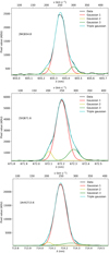 |
Fig. A.1. [N II] 654.8 (top), [S II] 671.6 (middle), and [Ar III] 713.6 (bottom) nebular lines fit with a triple Gaussian model. The model was extracted from the −5.1″ position in Fig. 5. |
Appendix B: Line plots
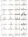 |
Fig. B.1. [O I] 630.0 nm, Hα, Ca II and Pa-13–16, and [Fe II] 1643.5 nm regions shown for S1–S5-A. For clarity, the [Fe II] 1643.5 nm region is enhanced. The confirmed MYSOs are boldfaced. We indicate the positions of the transitions with the red dashed lines (shifted with 260 km s−1 with respect to the heliocentric frame). The Paschen series and Br-8 lines are marked by yellow dash-dotted lines for clarification. The center of Hα is saturated due to nebular emission and was clipped. All narrow features are either telluric lines or residuals from the nebular or sky subtractions. |
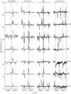 |
Fig. B.2. Fe II 1687.7 nm, H2 2121.8 nm, Brγ, and the 2–0 and 3–1 CO bandhead regions shown for S1–S5-A. All spectral regions are enhanced for clarity. All other lines and features are the same as in Fig. B.1. |
Appendix C: X-shooter magnitudes
Photometric upper limits in multiple bands computed from our X-shooter spectra.
All Tables
Lower limit luminosities and masses computed from X-shooter upper limits to the magnitudes.
Photometric upper limits in multiple bands computed from our X-shooter spectra.
All Figures
|
Fig. 1. 30 Dor nebula seen in the Y (blue), J (green), and Ks (red) bands with the VMC (Cioni et al. 2011). North is up and east is to the left. The observed X-shooter targets are labeled in white (see also Table 1). The central massive cluster R136 is the bright cluster of stars in the middle. |
| In the text | |
|
Fig. 2. Left: NIR color-magnitude diagram of our targets. With dots, we show the objects with accurate photometry (Cutri et al. 2003; Walborn et al. 2013) and, with arrows, we show the positions of objects based on a J > 19 lower limit. Errors on the data points were omitted for clarity but are typically ∼0.05 mag. In blue, we show the MYSOs confirmed in this work and, in black, the unconfirmed MYSO candidates. The green, red, and yellow dots indicate a MS, M-type giant, and WR star, respectively. The magenta dots are other LMC MYSOs (Ward et al. 2016; Reiter et al. 2019) and the cyan dots are SMC MYSOs (Ward et al. 2017; Rubio et al. 2018). The gray stars, squares, and diamonds are the MYSOs of Ramírez-Tannus et al. (2017), Bik et al. (2006), and Cooper et al. (2013) projected at a distance of 50 kpc, respectively. The ZAMS is shown as a black line, and the gray line indicates the position of O V stars of Martins & Plez (2006). The dashed black and gray lines are the reddening lines of an O3 V star for a RV of 3.1 and 5.0, respectively, where the crosses from left to right represent a visual extinction AV of 5, 10, 15, 20, 25, and 30 mag. We note that almost all our MYSO candidates are located above the reddening lines, implying a strong NIR excess. Right: NIR color-color diagram of our targets. The colors and symbols are the same as in the left plot. Most of our targets show evidence of a NIR excess due to their position at the right of the reddening lines. |
| In the text | |
|
Fig. 3. MIR color-color diagram showing the Spitzer/IRAC colors of our confirmed MYSOs (blue dots) and the unconfirmed MYSO candidates (black dots). The Spitzer/IRAC photometric points of the MYSO candidates and S3-K are from Walborn et al. (2013). The photometric points of R135 are from the Spitzer/SAGE catalog (Meixner et al. 2006). Following the classification scheme of Gutermuth et al. (2009), we indicate the Class I and Class II regions and the regions where the Spitzer/IRAC colors might include unresolved knots of shock emission or resolved structured PAH emission. |
| In the text | |
|
Fig. 4. Reduced 2D science frame of S4 as assessed from the pipeline. We show a single nodding position. The color indicates flux, where red and blue are high and low flux, respectively. The spatial position is with respect to the center of the slit. The figure is centered around the [S II] 671.6,673.1 nm lines (the two bright lines on the right) and the He I 667.8 nm line (the bright line on the left), all originating from the nebula. The three weak lines on the right are nebular Fe I lines. The continuum of S4 is visible in the lower part of the 2D frame. Additionally, some nebular continuum is visible. At the top, some weak continuum from an object not analyzed in this work. |
| In the text | |
|
Fig. 5. Variations in the [S II] 671.6 nm nebular line along the slit, which is modeled with a triple Gaussian model. The variations are shown for one of the nodding mode positions of S4. Top: variations in the peak flux of each GD along the slit. Middle: variations in the central wavelength or RV shift of each GD along the slit. Bottom: variations in σ of each GD along the slit. In the dark, lighter, and lightest vertical gray zones, we show the 1σ, 2σ, and 3σ seeing ranges of the object, respectively. For more information, see the text. |
| In the text | |
|
Fig. 6. Nebular and sky subtracted spectrum of S2 (black) and subtracted nebular contribution (red) centered around the Ca II IRT lines (indicated with vertical gray dashed lines). The nebular lines are Pa-11–19. Some residuals persist after the nebular subtraction. |
| In the text | |
|
Fig. 7. [O I] 630.0 nm, Hα, Ca II IRT and Pa-13–16, [Fe II] 1643.5 nm, Fe II 1687.7 nm, H2 2121.8 nm, Brγ, and the 2–0 and 3–1 CO bandhead regions shown for S4. For clarity, the [Fe II] 1643.5 nm, Fe II 1687.7 nm, H2 2121.8 nm, Brγ, and CO bandhead regions have been enhanced by a factor of 5 and 15, respectively. We indicate the positions of the transitions by the red dashed lines. The Pa series and Br-8 line are marked by yellow dash-dotted lines for clarification. The center of Hα was saturated due to nebular emission and has been clipped. All narrow features are either telluric lines or residuals from the nebular or sky subtraction. |
| In the text | |
|
Fig. 8. HST/WFPC2/F814W (red) +F555W (green) +F336W (blue) composite image (20″ × 20″) of the cluster field surrounding S5 (Walborn et al. 2002). North is up and east is to the left. The two nodding positions of the X-shooter slit are shown with the two black rectangles. We identify a total of six continuum sources in our observation, which we labeled A–F (indicated in red). Even though S5-E is not visible in this image, we still indicate its presumed location. |
| In the text | |
|
Fig. 9. Spectrum of S7-B centered around the three Pa lines. With the blue and red vertical dashed lines, we denote the locations of the blueshifted and redshifted peaks of emission at −355 km s−1 and −265 km s−1, respectively. The nebular counterpart of the Pa lines is indicated with the gray vertical lines at 250 km s−1. The region around ∼908 nm is a saturated [S III] nebular line. Other narrow features are either telluric features or residuals from the nebular subtraction. |
| In the text | |
|
Fig. 10. SEDs of S1–S5-F. The spectrum of each object is shown in black and has been smoothed by a factor of 100. The confirmed MYSOs are indicated in bold. The objects S5-B, S5-C, S5-D, and S5-F were not corrected for slit loss since we lack photometry of these objects. The telluric absorption bands around 1.1 μm, 1.5 μm, and 2.0 μm are clipped. Additionally, we clipped the spectrum above 2.25 μm due to sky variations and at short wavelengths for S2, S3, and S5-E due to the low flux of these objects. Literature photometric points are shown as the yellow diamonds (Parker 1992; Cutri et al. 2003; Kato et al. 2007; Walborn et al. 2013; Gaia Collaboration 2016). Upper limits are indicated with an arrow. With the dashed lines, we plotted a Castelli & Kurucz model for various AV. |
| In the text | |
|
Fig. 11. Same as Fig. 10, but for the objects S6-R135, where we clipped S6, S9, S10-A, S10-BC, S10-K, and S10-SW-B at short wavelengths. |
| In the text | |
|
Fig. 12. Left: NIR color-magnitude diagram of the upper limits derived from our X-shooter spectra (see Appendix C). Error bars are omitted for clarity, but they may be found in Appendix C; the typical error is ∼0.6 mag. The gray lines link our upper limit with the literature values (gray dots and arrows). All of the other lines are the same as in Fig. 2. We note that the color is composed of a subtraction of two upper limits and, therefore, it is uncertain. Right: optical color-magnitude diagram of the upper limit photometric points. In the VIS range, the photometric upper limits are well below the reddening line. Again the color is composed of a subtraction of two upper limits and, therefore, it is uncertain. |
| In the text | |
|
Fig. 13. Luminosity of Brγ plotted against the absolute K-band magnitude. Various MYSO samples in the LMC, SMC, and our Galaxy are overplotted. With the gray and red lines, we indicate the empirically derived relations of Cooper et al. (2013) and Ward et al. (2017) for our Galaxy and the SMC, respectively. |
| In the text | |
|
Fig. A.1. [N II] 654.8 (top), [S II] 671.6 (middle), and [Ar III] 713.6 (bottom) nebular lines fit with a triple Gaussian model. The model was extracted from the −5.1″ position in Fig. 5. |
| In the text | |
|
Fig. B.1. [O I] 630.0 nm, Hα, Ca II and Pa-13–16, and [Fe II] 1643.5 nm regions shown for S1–S5-A. For clarity, the [Fe II] 1643.5 nm region is enhanced. The confirmed MYSOs are boldfaced. We indicate the positions of the transitions with the red dashed lines (shifted with 260 km s−1 with respect to the heliocentric frame). The Paschen series and Br-8 lines are marked by yellow dash-dotted lines for clarification. The center of Hα is saturated due to nebular emission and was clipped. All narrow features are either telluric lines or residuals from the nebular or sky subtractions. |
| In the text | |
|
Fig. B.2. Fe II 1687.7 nm, H2 2121.8 nm, Brγ, and the 2–0 and 3–1 CO bandhead regions shown for S1–S5-A. All spectral regions are enhanced for clarity. All other lines and features are the same as in Fig. B.1. |
| In the text | |
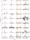 |
Fig. B.3. Same as in Fig. B.1, but for S5-B–S7-B. |
| In the text | |
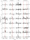 |
Fig. B.4. Same as in Fig. B.2, but for S5-B–S7-B. |
| In the text | |
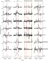 |
Fig. B.5. Same as in Fig. B.1, but for S8–S10-SW-B and R135. |
| In the text | |
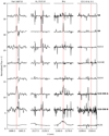 |
Fig. B.6. Same as in Fig. B.2, but for S8–S10-SW-B and R135. |
| In the text | |
Current usage metrics show cumulative count of Article Views (full-text article views including HTML views, PDF and ePub downloads, according to the available data) and Abstracts Views on Vision4Press platform.
Data correspond to usage on the plateform after 2015. The current usage metrics is available 48-96 hours after online publication and is updated daily on week days.
Initial download of the metrics may take a while.