| Issue |
A&A
Volume 635, March 2020
|
|
|---|---|---|
| Article Number | A115 | |
| Number of page(s) | 16 | |
| Section | Interstellar and circumstellar matter | |
| DOI | https://doi.org/10.1051/0004-6361/201937025 | |
| Published online | 24 March 2020 | |
The ambiguous transient ASASSN-17hx
A possible nova impostor
1
INAF-OATS,
Via G.B. Tiepolo 11,
34143
Trieste,
Italy
e-mail: This email address is being protected from spambots. You need JavaScript enabled to view it.
2
Dipartimento di Fisica, Universitá di Pisa, Largo Enrico Fermi,
Pisa, Italy
3
Mullard Space Science Laboratory, University College London,
Holmbury St Mary,
Dorking,
Surrey
RH5 6NT,
UK
4
ARAS group, Mirranook,
Armidale,
NSW,
Australia
Received:
30
October
2019
Accepted:
30
January
2020
Abstract
Aims. Some transients, although classified as novae based on their maximum and early decline optical spectra, cast doubts on their true nature, and raise the question of whether nova impostors might exist.
Methods. We monitored a candidate nova that displayed a distinctly unusual light curve at maximum and early decline through optical spectroscopy (3000–10 000 Å, 500 < R < 100 000) complemented with Swift UV and AAVSO optical photometry. We use the spectral line series to characterize the ejecta dynamics, structure, and mass.
Results. We find that the ejecta are in free ballistic expansion and have a typical classical nova structure. However, their derived mass is at least an order of magnitude higher than the typical ejecta masses obtained for classical novae. Specifically, we find Mej ≃9 × 10⁻³ M⊙ independent of the distance for a filling factor ε = 1. By constraining the distance we derived ε in the range 0.08–0.10, giving a mass 7 × 10⁻⁴ ≲ Mej ≲ 9 × 10⁻⁴ M⊙. The nebular spectrum, characterized by unusually strong coronal emission lines, confines the ionizing source energy to the range 20–250 eV, possibly peaking in the range 75–100 or 75–150 eV.
Conclusions. We link this source to other slow novae that show similar behavior, and we suggest that they might form a distinct physical subgroup. The sources may result from a classical nova explosion occurring on a very low-mass white dwarf or they may be impostors for an entirely different type of transient.
Key words: stars: mass-loss / novae, cataclysmic variables
© ESO 2020
1 Introduction
ASASSN-17hx (also called nova Sct 2017; hereafter 17hx) was discovered on Jun 19.41 UT as a candidate bright nova (Stanek et al. 2017). Spectroscopic confirmation came one day after the announcement (Kurtenkov et al. 2017a) together with its CTIO spectral classification (Williams et al. 1991, 1994). Reports of the 17hx light curve and spectral variations filled the ATels for about 3 months (Williams & Darnley 2017; Saito et al. 2017; Berardi et al. 2017; Munari et al. 2017a,b,c; Pavana et al. 2017; Kuin et al. 2017; Kurtenkov et al. 2017b; Guarro et al. 2017), while the observations continued to build a substantial data set. In an attempt to make sense of the peculiar light curve of ASASSN-17hx, we collected spectra, in particular high-resolution spectra, for 2 yr after discovery. In this paper we present those spectra and our results. In what follows we make no assumptions about the classical nova (CN) nature of 17hx. We show that a central object governs the radiative budget of the ejecta, and demonstrate that the spectra arise from a freely expanding gas in ballistic motion, as in CNe. Nevertheless, this transient is dissimilar to CNe in other significant aspects.
2 Observations and data reduction
The full characterization of a CN or an optical transient requires long-term monitoring, preferably for several years. Our spectroscopic campaign extended for 2 yr. The early decline phase was fortuitously monitored by Ultraviolet and Visual Echelle Spectrograph (UVES; Dekker et al. 2000) at the Very Large Telescope (VLT) within an independent program (299.D-5043 and 0100.D-0621, PI Molaro). The UVES sequence consists of four epochs spread over two months starting from two months after discovery. They sample (see light curve in Fig. 1) two distinct optical photometric minima and the second maximum. The instrument setups and total integration times are listed in Table A.1. The UVES data were retrieved from the archive and processed using the Esorex+Gasgano pipeline v5.9.1. Flux calibration was achieved using the instrument response curve produced by the observatory (no dedicated spectrophotometry was obtained during the observing nights). Due to the narrow slit employed (see Table A.1) for the science and the default 5″ slit adopted by the observatory for the calibration program, the UVES spectra are affected by unaccounted slit losses.
The early decline of 17hx was intensively monitored by the ARAS group1 for over five months with low- and mid- to high-resolution spectroscopy. We selected from the database the spectra having R ≥ 9000 for inspection of the Hα profile2, and the low-resolution (R < 1000) flux calibrated spectra for inspection of the spectral energy distribution (SED) and for comparison with the UVES spectra. Epochs, spectral resolution, and exposure times for each of the selected ARAS spectra are reported in Table A.2. We note that the ARAS data are available in reduced form and that the data reduction process used by the group followed the standard procedure.
Late spectra were taken ~9 and 11 months after outburst by one of us (TB) in low-resolution mode (LISA spectrograph on a 0.28 m Celestron telescope) together with broadband photometry (B, V) and were complemented with mid-resolution spectra taken at the Heidelberg robotic telescope TIGRE (Telescopio Internacional de Guanajuato Robotico Espectroscopico) with HEROS (Heidelberg Extended Range Optical Spectrograph) almost 15 months after outburst (see Table A.3). We note that LISA spectra were reduced following the same standard procedure outlined in the ARAS web pages and calibrated in flux through simultaneous photometry observations. The HEROS spectra, although pipeline processed following standard procedures, were not flux calibrated.
The last sequence of spectra consists of two NOT (Nordic Optical Telescope)/FIES (FIber fed Echelle Spectrograph; Telting et al. 2014, Frandsen & Lindberg 1999) spectra taken about two years after outburst with the aim of observing the optically thin nebular phase of the object (see Table A.4). The data were reduced with the instrument pipeline at the telescope. The observing strategy envisioned for the instrument did not include background subtraction (there is no dedicated sky-fiber in mid-resolution mode) since it is expected to be insignificant. We verified this with a 900 s sky exposure in which both the exposed and the masked part of the CCD showed the same count level, and with the science exposure whose inter-order background roughly matched that of the sky exposure. We therefore ascribe only a few percent uncertainty to the flux calibration process in the absence of sky subtraction with FIES. We note that the largest systematic effect is introduced by the reddening correction (see below).
Of the two FIES epochs, the May spectrum was contaminated by stray light (J. Telting, priv. comm.) that affected the background level redward of 6400 Å. Therefore, any physical parameter derived in the following sections relies on the data taken during the July run, which happened after the installation of a new light-leak baffle around the spectrograph shutter. During the July run, however, we experienced a color loss between the first exposure and the following two exposures. Specifically, we found up to 30% loss in the blue part of the spectrum (Hγ, 4363Å), only ~5% at Hα, and 7065 Å in the line flux of the second and third exposure compared to the first. This happened because the spectrograph atmospheric dispersion corrector (ADC) is set at the beginning of the sequence and is not updated during subsequent exposures. Since the target crossed the meridian after ~2/3 of the first exposure, the first exposure should have suffered differential color losses as well. Thus, our derived density (see Sect. 6) is only a lower limit even if we use only the first spectrum in the calculation.
 |
Fig. 1 Top panel: AAVSO V light curve together with the epoch of the UVES observations (blue lines), the ARAS high-resolution un-calibrated and low-resolution flux calibrated spectra (green dotted and solidlines, respectively), the LISA and HEROS observations (red lines), and the FIES spectra (cyan lines). Middle panel: AAVSO B, R, and I light curves together with Swift UVOT UVW1 (λc =2600 Å), UVM2 (λc=2246 Å), and UVW2 (λc1928 Å). Bottom panel: color light curve: (B–V), (V –R), and (V –I). Error bars ≥0.2 mag in the color light curves were arbitrarily set whenever either the V or the paired broadband photometry did not have an associated error bar. Colors were computed every time the V and broadband filter were taken within 3 h observations. |
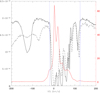 |
Fig. 2 Comparison of the temperature profile of the H I 21 cm (red line) with the Na I (black solid line) and Ca II K (black dashed line) interstellar absorption profiles. The two vertical blue dotted lines mark the limits for the column density calculation (see Sect. 2 for details). Units of flux (erg s−1 cm−2 Å−1) and temperature (K) are on the left and right axis, respectively. |
Reddening correction of the spectra
The high signal-to-noise ratio and high resolution of the UVES spectra allow us to use the interstellar absorptions to estimate the reddening. The spectra show multiple saturated Na I D and Ca II H&K interstellar components, indicating that 17hx is significantly reddened. The saturation of the Na I D absorption lines prevent using the Munari and Zwitter 1997 EW(Na I D)-E(B-V) relation. The much weaker and resolved K I absorptions are, however, blended with telluric absorptions so that using the analogous relation for the potassium resonance line provides only a lower limit: E(B − V) > 0.4 mag.
Figure 2 shows the antenna temperature profile of the neutral H from the LAB 21 cm maps (Kalberla et al. 2005) together with the interstellar absorption from Na I and Ca II in the local standard of rest (LSR) frame. The good match in the structures support using the H I column density to estimate the E(B − V) following Bohlin et al. (1978). Specifically, integrating the H I temperature in the velocity range [−20,+125] km s−1 (i.e., the velocity range spanned by the sodium and calcium absorptions), we derive E(B − V) =0°.71±0.02 mag, where the uncertainty is purely statistical. This is the reddening we apply to all spectra in the following analysis. We note that the adopted E(B − V) agrees with the values derived by Munari et al. (2017a, 0.68 mag) and by Kuin et al. (2017, 0.8±0.1 mag), within the errors.
All figures in this work were created using the observed spectra (i.e., not corrected for reddening). We applied the reddening correction ahead of any physical parameter derivation (Sect. 6.2).
3 Data analysis: the light curves
Figure 1 shows the 17hx light curves in the filters B, V, R, and I, obtained from the AAVSO database (Kafka 2019), together with the epochs of the spectroscopic observations listed in Tables A.1–A.4 (top and middle panels). The bottom panel of Fig. 1 displays the color curves. The middle panel of Fig. 1 also displays the sparse UV photometry obtained by Swift. The UV photometry is also listed in Table A.5, including the data points that are outside the plotted time intervals.
The optical photometry shows that the 17hx light variations are exceptional in both amplitude and timescale. Brightness variations of CNe during maximum rarely exceed 1–1.5 magnitudes, while their timescales never extend beyond a couple of weeks. Here the amplitudes are >2 mag on a timescale of 1–2 months. The amplitudes are greater in the V band.
The UV photometry, instead, is possibly suggestive of flux redistribution since the UVM2 flux displayed a drop during the first ~50 days, while the optical flux increased. Unfortunately, because of the limited number of UV observations, we cannot draw a firm conclusion. To date, flux redistribution has been convincingly shown only for nova Cyg 1992 (Shore et al. 1994).
The color light curves (Fig. 1, bottom panel), show B–V, V − R, and V − I colors that are in low-amplitude anti-phase with respect to the broadband light curves: 17hx seems redder during the minima than the maxima. However, spectroscopy shows that the continuum SED is redder at maximum than at minimum (see Sect. 4, Figs. 3 and 9). The color variation and in particular the V –I and B–V color maxima are driven by the strong emission lines during the photometric minima. Although less pronounced, similar behavior is not uncommon among classical novae (e.g., nova Cen 2013 and nova Sgr 2015b; see the AAVSO light curves for the photometry and Mason et al. 2018 for nova Cen spectroscopy; nova Cen and nova Sgr 2015b spectra are publicly available in the ESO archive), and highlight the potentially misleading inferences from photometry alone.
4 Data analysis: early spectroscopy, the optically thick stage
4.1 High-resolution UVES spectra
The four UVES spectra cover the first decline and minimum after the first optical maximum, the second maximum, and the decline afterthe fourth maximum (see Fig. 1). They therefore permit a comparison in great detail (R ≥60 000) of spectral characteristics at the different photometric states providing important information about the gas kinematics and physics.
At all epochs, the emitting gas is dominated by H I (from the Balmer and the Paschen series, see Fig. 3) and low ionization potential metal lines, mainly Fe II (e.g., Revised Multiplet Table, RMT, 73, 40, 46, 55, 56, 49, 48, 41, 42, 35, 47, 37, 38, 27, and 28), but also Ca I (RMT 2) and II (H&K and the near-IR, NIR, triplet). Non-metal transitions are also present, for example O I (RMT 1 and 4), Si II (RMT 2), and He I. There are no forbidden transitions since, as we show later, the densities at these stages are very high.
Apart from that, the three minimum/decline spectra are similar to each other, but are very different from that at maximum. In particular, the minimum and decline spectra display a flat continuum, strong emissions with rectangular shape profile partially resolved into numerous structures (i.e., “castellated” tops), and weak or absent absorption components. Conversely, the maximum spectrum displays a redder continuum, and weak emission components with a smooth profile and strong P Cyg-like absorptions (see Figs. 3–5). The difference in the emission line profiles suggests that during the minima only a small number of structures contribute to the emission component, while at the maximum many more structures contribute to the emission creating a blended profile.
More importantly, the ionization degree of the emitting gas changes with the photometric oscillations and is higher at the minima than at the maximum. This is best illustrated by the changes in the He I lines (see Fig. 6). The weakness of the emission component during the maximum indicates reduced He+ recombination, yielding insufficient emission measure for detection. The velocity displacement of the absorption, instead, indicates that during the maximum the absorption (of high-energy photons) is confined to the low-velocity regions of the gas. In other words, larger volumes and higher velocities are involved in the He+ recombination during the minima.
The Ca transitions confirm this trend (see Fig. 5). The strengthening of the narrow absorption at approximately −460 km s−1, together with the appearance of a broad and deep absorption component at approximately −660 km s−1 in both Ca I and Ca II transitions indicates more neutral Ca and Ca+ at maximum than at minimum. During the photometric minima the Ca is largely twice ionized, given that the Ca+ ionization potential (IP) is ≲12 eV (i.e., less than that of H0 and Fe+, and much less than that of He0).
Neutral silicon, an intermediate ionization potential element (IP ~ 8 eV), displays analogous behavior to the Fe II transitions (see Fig. 7). Like the optical iron multiplets, the Si II doublet is a transition between two excited levels, specifically 4s and 4p. The lower level 4s is connected to the ground state by resonance transitions (λ1533,1526). To produce λ6347,6371 emissions and absorptions, the resonance UV transition must be optically thick with low collisional de-excitation of the 4p level. This suggests an electron density ne ≃7 × 1014 cm−3. Again, the strong broad absorption visible at maximum suggests that at this time there is more Si+ than at minima when it is likely twice ionized. The Si II disappears in the last UVES spectrum, suggesting that the gas has diluted to the point that the UV doublet λ1553,1526 is no longer optically thick, and is thus incapable of overpopulating the 4s level. We exclude that the Si+ further ionized into Si2+ since the IP for Si+ is about the same as Fe+ (~16 eV) and Fe II transitions are still present in the last UVES spectrum.
Finally, O I is detected only in the RMT triplets (1) and (4). They are interesting for their remarkably different profiles. The RMT triplet (1) (λ7772,7774,7775) forms mainly via recombination cascade of O+. It can display absorption components because its lower level leads to the ground state through an intercombination transition. In contrast, the RMT triplet (4) (centered around λ8446), is mainly produced by optically thick H Lyβ transition that pumps the upper level of the OI λ1025 and, by cascade, populates the upper level of the λ8446 triplet (Keenan and Hynek 1950) in combination with an optically thick O I λ1302 (which is responsible for the overpopulation of the lower level 3S of the triplet and explains the occasionally strong absorption component). Neutral oxygen has nearly the same ionization potential energy as H (~13 eV) and the ~λ7774 triplet has asimilar profile to the Balmer lines (see Fig. 8, top panel, where the triplet is plotted together with the Hδ transitions).The hydrogen and oxygen recombine together with just small local differences. The λ8446 triplet, in contrast, shows only emission whose profile matches the Fe II and Si II transitions at minima, but displays almost pure absorption at maximum. Like Fe II and Si II, the λ8446 triplet results from UV pumping that is favored by the high UV opacity of the “iron curtain.”
In summary, at minimum the ionization state of the gas increases displaying stronger structured emission profiles and higher velocity absorptions in the high IP energy transitions, but null or weak absorption in the low IP energy transitions. In contrast, at maximum the gas recombines, the average emission measure within each transition diminishes, and the photoexcit- ation is confined to the low-velocity range (the lower deep absor- ptions of the maximum P Cyg profiles).
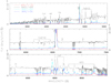 |
Fig. 3 Four high-resolution spectra taken at VLT/UVES. The spectra have been split in three panels where there is the wavelength gap induced by the dichroic or the detector mosaic (red arm only). Photometric state and age since discovery (in days) are color-coded in the upper panel. The Hα line is saturated in all UVES spectra. The spectra in the figure have not been corrected for reddening. |
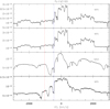 |
Fig. 4 Evolution of the Fe II λ5169 (RMT 42) transition. Y -axis units are in erg cm−2 s−1 Å−1. The blue and red dotted lines indicate the velocity of the persistent narrow absorption (see Sect 4.1) and of the He I absorption in the first UVES spectrum, respectively, for a comparison (see text for details). The photometric state (min, max) of each spectrum is indicated within each panel. |
Narrow absorption at around −460 km s−1
All the UVES spectra display a narrow absorption at approximately −460 km s−1 that is present in all transitions (H I, Fe II, Ca I and Ca II, Si II, K I, O I) except those of He I (see the blue dotted line in Figs. 4, 5, 7, and 8). It also persists when other absorption components disappear. Although this could be consistent with circumstellar gas, we exclude this explanation for the following reasons. Absorptions from excited and/or metastable levels (as in the case of Fe II and Ca II NIR) would imply unusually high column densities. Similarly, the detection of the narrow absorption in the O I λ7774 and H Balmer transitions would require that the central object is sufficiently powerful to ionize the circumstellar environment that is more than 114 AU = 2.4 × 10⁴ R⊙ away from the transient3, since it is dynamically undisturbed at day 132. Figures 4 and 5 and EW measurements show that the narrow absorption is stronger at maximum and weaker at minimum (i.e., it varies responding to the radiation field in phase with the rest of the ejecta). This requires similar physical conditions in the narrow absorption region and the ejecta. Hence, the narrow component originates in the ejecta and its persistence informs about the gas kinematics, specifically that it is in ballistic expansion (v ~ r) as typical for explosive processes. The emitting gas is not a wind and is not a pulsating pseudo-photosphere, but an ejecta similar to CNe.
4.2 Low-and medium-resolution ARAS spectroscopic sequences
The ARAS spectra listed in Table A.2 support and extend our finding from the UVES spectra. Figure 9 shows the evolution of the SED, uncorrected for reddening, and of the emission lines across the first photometriccycle. 17hx displays a flat continuum and strong emission lines with weak or no (i.e., not resolved) P Cyg-like absorptions during the minima and the declining states. Instead, it has a redder continuum and strong P Cyg during maxima and the rising state.
The similarity of the line profiles at minimum and decline or maximum and rising phases is more evident in Fig. 10, which shows the evolution of Hα, Hβ, He I λ5876 (blending at any time with Na I D both of ejecta and interstellar origin), and Fe II λ5169. The spectra are normalized to the continuum. What emerges from the figure is the following:
- 1
the emission line component in each transition at minimum is always at least an order of magnitude stronger than at maximum;
- 2
the Hα and Hβ profiles are remarkably different (especially from day +74 on), indicating that the lines are very optically thick;
- 3
within each cycle the line profiles change from a strong emission flanked by a weak P Cyg absorption to a weak emission with a strong P Cyg absorption. However, on subsequent cycles the emission component both strengthens and broadens;
- 4
the emission profiles differ systematically in structure depending on the photometric state and show rectangular and castellated forms, especially in the low ionization potential energy transitions, during the minima and smoother and featureless profiles at maxima.
- 5
high ionization potential energy species (e.g., He+ which recombining produces He I lines) display no emission during maxima and detectable emission during minima. In addition, their absorption component (which is always single and shallow) moves outward and inward at minima and maxima, respectively.
Both Figs. 9 and 10 show that the degree of ionization of the emitting gas increases at minima with respectto maxima, while the continuum becomes bluer.
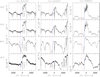 |
Fig. 5 Evolution of the Ca I and Ca II line profiles (see text for details). The emission centered at about +500 km s−1 in the first column (Ca I panels) is from Fe II RMT 27. The arrow in the third panel from the top indicates the second broad absorption from Ca I λ4226. The Y -axis units are in erg cm−2 s−1 Å−1. The blue and red dotted lines indicate the velocity of the persistent narrow absorption (see Sect. 4.1) and of the He I absorption in the first UVES spectrum, respectively. The photometric state (min, max) of the spectra is indicated on the left of each row. |
5 Data analysis: late low- and medium-resolution spectroscopy, the transition stage
The two LISA low-resolution spectra taken during March and May 2018, 284 and 344 days after outburst, are similar to each other and show a highly opaque emitting region (see Fig. 11, top panel). The Hα line is one order of magnitude stronger than Hβ in the observed spectrum (10−10 versus 9 × 10⁻¹² erg cm−2 s−1 Å−1, respectively), or a factor 5.3 stronger when dereddened. The strongest emission lines after the Balmer series are He I, especially the triplets (e.g., λ5875 and 7065 Å), while He II λ4685 and the Bowen blend at 4640 Å are weakly present. Weak forbidden transitions, such as [Ne III] λ3968, [N II] λ5755 and [O III] λ5007, 4959, and 4363, are also present and evince the thinning of the gas. The [O III] emissions are particularly weak and the λ5007 is blended with the strong He I λ5015 producing aline centered at 5011 Å. Even neglecting the He I contribution to such a blend, the electrondensity resulting from the [O III] line ratio (e.g., Osterbrock 1989, adopting Te ~10 000 K) is >107 cm−3, which is much greater than the critical value (~7 × 105 cm−3 for the [O III] RMT 2 and a few × 103 cm−3 for the RMT 1; Osterbrock 1989). Other weak emission lines are [O I]λ6300,6364 and possiblySi II λ6347. Weak unidentified emission lines are detected at 5159A, 5267, and 5315 Å, which cannot be coronal emission from [Fe VI], [Fe V], and [Fe VII], respectively, since they are absent in the following HEROS spectra. They cannot be Fe II since the stronger multiplets (e.g., multiplet 42, 48, 49) should also be present; they are not, nor are there any detectable [Fe II] transitions.
The higher resolution HEROS spectrum (day 462, August 20, 2018; see Fig. 11, bottom panels), although not flux calibrated, can be used to confirm the line identification of the LISA spectra and that the unidentified lines have disappeared. The higher resolution spectrum also reveals some differences in the line profiles. In particular, the forbidden transitions display stronger wings (up to ~±1200 km s−1), indicating that they arise in the high-velocity, lower-density peripheral regions of the ejecta.
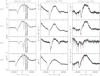 |
Fig. 6 Evolution of the He I (triplet and singlet) transitions (see text for details). The Y-axis units are in erg cm−2 s−1 Å−1. The reddotted line indicates the velocity of the absorption component at the first epoch: ~1050 km/s. The photometric state (min max) is indicated on the left of each row. |
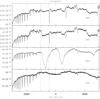 |
Fig. 7 Evolution of the Si II doublet (RMT 2) transition (see text for details). The Y-axis units are in erg cm−2 s−1 Å−1. The colored vertical lines are identical to those in the previous figures. The photometric state (min, max) of the spectra is indicated within each panel. |
6 Data analysis: late high-resolution spectroscopy, the optically thin stage
The two FIES spectra, taken about 2 yr after outburst, are separated by only ~2 months. The spectra are quite similar and display the same species and transitions, in line with the slow evolution of 17hx. We show only the July 2019 spectrum in Fig. 12 since it was not contaminated by scattered light (see Sect. 2). In both spectra the strongest emission lines are still those of the H Balmer series. The forbidden transitions, however, have increased in relative intensity with respect to the 2018 observations, especially the λ3869 of the [Ne III](1) doublet that is among the strongest lines in the spectrum. The He II λ4686 emission line is also one of the strongest lines (see Fig. 12). The [O III] lines are present but weak. We also identify numerous weaker emissions from He I (triplet and singlet) and highly ionized metals: [Fe VI] λ5177, 5147, 5236, and 5678; [Fe VII] λ6086, 5276, and 5720; [Ca V] λ5309 and 6086 (blending with [Fe VII]). [Fe X] λ6373 may be weakly present in a blend with other emissions of difficult identification. [N II] λ5755 is present but weaker than He I λ5876 and [Fe VII] λ5720, while the fractional contributionof [N II] λ6584,6548 to Hα is insignificant. Other forbidden transitions are from [Ar III] λ7136, 7751, [Ar IV]λ7169, and [Ar V] λ7006. There are a few lines which we are unable to identify, in particular λ6638 and 6487, although they are well isolated and not in a blend. We detect no C II or C III transitions and only very weak C IV λ5801,5812.
The two FIES spectra confirm that 17hx entered an optically thin stage since the line profiles remain unchanged in the two epochs (see Fig. 13). However, the ejecta are not yet in nebular conditions, as we show in Sect. 6.2.
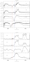 |
Fig. 8 Evolution of the O I triplets (RMT 1, top, and 4, bottom). Triplet (1) is resolved in the narrow absorption at approximately −460 km s−1. Together with triplet (1) we overplot the Hδ profile forcomparison (gray line) (see text for details; the H line has been arbitrarily offset in each subpanel; in the bottom subpanel it has also been scaled by a factor 0.5). The blue line of the Ca II triplet is included in the bottom panel; it shows similar behavior to the O I RMT 4. The Y -axis units are in erg cm−2 s−1 Å−1. The colored vertical dotted lines have the usual meaning. The photometric state (min, max) of each spectrum is indicated in each subpanel. |
6.1 Central source SED constraints
We can infer a few important things from the comparison of the 2019 FIES spectra with those from 2018, and the inter-comparison of the FIES spectra. The strengthening of the He II emission together with the appearance of the coronal lines in the later spectra indicates that the ionization degree has increased and that the ejecta is exposed to radiation between the extreme UV and the low energy X-ray. The strengthening of the [O III] emission lines, instead, indicates that the density has decreased. The LISA and HEROS observations demonstrate that in 2018 the density of the expanding gas was still too high to display a significant increase in ionization and that the ejecta was barely beginning to “thin”. Conversely, in 2019 the density of the ejecta must have decreased enough to become substantially ionized.
Although we cannot compare the relative intensities at the two 2019 epochs along the whole wavelength range of the FIES spectra because of the scattered light contamination (May spectrum) and color losses (July and possibly May spectra), we can compare them where their continuum matches (4600–5200 Å). This is sufficient to establish that the He II line (λ4686) intensity remained constant or slightly increased, that [O III]λ5007 slightly decreased, and Hβ more so, while [Fe VI]λ5147,5177 and [Fe VII]λ4942 remained constant. The weakening of the hydrogen emission together with the constancy of the He II and coronal lines, requires that the ionizing source is still active.
The coronal line emission profiles are at least as broad as the permitted and the nebular transitions. They also display the same structures and their profiles are unchanged between the two epochs (Fig. 13). This precludes the role of shocks in their formation. Shock excitation of different regions of the ejecta, or between the ejecta and any circumstellar material, should be localized at the colliding region and therefore display marked differences between coronal and permitted or nebular line profiles.They should also produce changing profiles with time as the shock propagates. That said, we can constrain the incident spectral distribution of the ionizing source using the coronal lines and transitions from elements that present a range of ionization (e.g., in addition to [Fe VI], [Fe VII], and possibly [Fe X], He I and He II4). The corresponding ionization potential (IP) values are in the range 75–230 eV for iron and 24–54 eV for helium. Since [Fe X] is very weak and since we certainly do not detect [Fe XIV] or [Fe XI], we place the upper cutoff of the ionizing source in the range 200–250 eV (the IP for Fe10+ is ~260 eV). The stronger [Fe VII] and [Fe VI] transitions compared to the (putative) [Fe X] (which has a transition probability ~100 times greater) requires substantial flux from the ionizing source in the range 75–100 eV. It cannot be much below that otherwise He+ would be over-ionized (although the fraction of doubly ionized helium is increasing). On the low-energy side, we place the low cutoff at about 20 eV in order to have H just recombining (it weakens between May and July because of expansion) and He ionizing.
6.2 Ejecta mass and filling factor
The invariant structures in the line profile (both forbidden, i.e., optically thin transitions by definition, and in the Balmer lines) indicate that the gas is in free expansion and optically thin. The observed decrease of the Hβ emission (−15 to 20%) in consistent, within the errors, with the density dropping with time, t, as t−3 (−20 to 25%) typical of freely expanding gas in ballistic motion and of CNe. Hence, we can constrain the electron density from the [O III] lines as we have done for late nebular spectra of CNe (e.g., Shore 2013a,b, 2016; Mason et al. 2018). We are aware, however, that the relative intensity of the [O III] components in 17hx indicates that collisional de-excitation is not negligible and the density must exceed the critical density. We verified that for spectra of CNe whose [O III] emission had similar relative strength to 17hx, the derived ejecta mass is smaller than that computed from later spectra because of the collisional damping of the diagnostic lines. We therefore used the [O III] diagnostic to estimate the nebular density and constrain the ejecta mass, being aware that the first is likely underestimated because of the wavelength dependent flux losses (see Sect. 2) and the latter will be underestimated because of collisional damping of the forbidden transitions. Figure 14 shows the nebular density derived using the [O III] diagnostic for an assumed electron temperature of Te ~10 000 K (Osterbrock 1989, Chapter 5), velocity bin per velocity bin. Since the 4959 Å component is heavily blended with [Fe VII] we disentangled its contribution using the 5007 Å profile scaled by the ratio of their transition probability (2.9 in NIST). We find an average density of ~3.5–4 × 107 cm−3 with some minor fluctuation across most of the line width.
We constrained the ejecta’s geometry by mimicking the emission line profiles with our bicone code, which is a Monte Carlo simulation that scatters, in ballistic but otherwise random distribution, 10–30 thousand points (each representing individual ejecta structures) within a biconical geometry that can vary in opening angle, thickness, and orientation (Shore 2013a; Mason et al. 2018). The closest matching model has maximum velocity vmax=1500 km s−1, high inclination (~80 deg), and a wide opening angle (~140 deg), and is geometrically thin compared toother novae (i.e., vmin ~50–60% of vmax compared to ~30% for nova Mon 2012, nova Del 2013, and nova Cen 2013; see Shore 2013a, 2016, and Mason et al. 2018, respectively). With the density, its radial gradient and the geometry of the ejecta we can derive the ejecta mass upper limit for a filling factor of unity: Mej ≃ 9 × 10⁻³ M⊙. We emphasize that, although this estimate is model dependent since it requires knowing the departure from sphericity, it is independent of distance. We know, however, that the filling factor, ε, is <1 since the structures in the line profiles indicate fragmented ejecta. The question is whether ε can reduce the ejecta mass to the range of normal CNe. To obtain ε we need the absolute luminosity of a pure recombination line, Hβ, sampling the same volume as the nebular diagnostic. This requires knowing the distance. The observed line of sight of H I 21 cm emission is optically thin, and its matching profile with the atomic interstellar absorption lines (see Fig. 2) indicates that 17hx is fairly distant. Using the Galactic rotation curve, for the highest observed radial velocity of the 21 cm emission and of the Na I and Ca II absorptions (vLSR ≃120 km s−1), we obtain a line of sight distance of ≈ 7.6 kpc. Moreover, the total reddening inferred from infrared maps in 17hx direction is E(B − V) = 1.5 mag (Schlafly & Finkbeiner 2011) and is about twice our derived value (see Sect. 2). Considering that most of the dust is confined within the solar circle, our derived E(B − V) is consistent with 17hx being located at about the same distance as the Galactic center. We therefore take 7.6 and 8.5 kpc as the lower and upper limits for the distance to constrain ε. The dereddened Hβ integrated flux is L(Hβ)obs = 2.04 × 10⁻¹¹ erg cm−2 s−1 Å−1 (=1.95 × 10⁻¹² in the original extinct spectrum). As in our previous studies, we define ε ≡ L(Hβ)obs/L(Hβ)predicted, where the prediction is based on our computed ne and volume from the models, assuming case B recombination. Case B recombination may overestimate the real recombination rate, given the high densities of the ejecta. For the distance bounds we obtain 0.08 ≲ ε ≲ 0.1, yielding ejecta mass in the range 7 × 10⁻⁴ ≲ Mej ≲ 9 × 10⁻⁴ M⊙. These estimates are at least an order of magnitude higher than the highest values derived for CNe, especially those we have similarly analyzed.
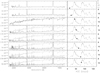 |
Fig. 9 Sequence of low-resolution flux calibrated ARAS spectra, together with their position in the V -band light curve. The Y -axis units are in erg cm−2 s−1 Å−1 and mag on the left and right side, respectively. Each panel plots in gray the previous spectra for easier comparison. |
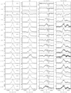 |
Fig. 10 Evolution across four min-max cycles of the H, He I, and Fe II lines, representing respectively intermediate, high, and low ionization potential energy atoms. The exact photometric state of each spectrum is indicated in the panels of the first column; the age (in days) is on the left. The He I transition is contaminated by Na I D both of interstellar and ejecta origin. The Na I D transition (emission and absorption) originating in the ejecta is particularly evident in the spectra taken between day 82 and 101. |
7 Discussion and conclusions
ASASSN-17hx resembles a CN in some properties, but it is strikingly anomalous relative to the majority of CNe in a number of other aspects. Specifically, 17hx can be explained with the same dynamical and bolometric physical model we have advocated for CNe (Shore 2012, 2013a, 2016; De Gennaro Aquino et al. 2014; Mason et al. 2018) that does not require a wind or dynamically interacting multiple ejections. The light curve results from redistribution and reprocessing of the photons emitted from a central source as they pass through the ballistically expanding ejecta. The ejecta are structured as in CNe. The spectra developed, analogously to all CNe, from an initial opaque phase, through a semi-opaque transition phase, to a transparent nebular one. The oddities are in the details.
The early outburst was dominated by large oscillations that for amplitude and the interval between peaks are unusual for CNe. The nebular spectra displayed unusual line strength in the coronal emissions. The estimated ejecta mass is higher or much higher than typical CNe and this, combined with the observed velocity, implies a larger kinetic energy than typical CNe. We now discuss eachof these points in detail.
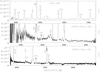 |
Fig. 11 LISA (top panel) and HEROS (mid and bottom panels) spectra of 17hx ~1 yr after outburst and/or discovery. The LISA spectrum is in units of erg cm−2 s−1 Å−1 and uncorrected for reddening, while the HEROS spectrum is in arbitrary units. The spectrograph and the age of the spectrum are indicated in each panel. |
7.1 Light curve oscillations
Our early spectroscopy demonstrates that the 17hx optically thick phase oscillations were accompanied by changes in the degree of ionizationof the expanding gas, with higher ionization observed at the minima than at maxima. Thus, the photometric and spectroscopic changes can result from alternating ionization and recombination waves propagating through the expanding gas as the underlying source varied in brightness and SED (or hardness). When the incident flux is higher or harder, the pseudo-photosphere recedes, the continuum peaks at short wavelengths, the visible and the NIR fluxes drop, the iron peak elements ionize, and He I is excited. This is a photometric minimum. If the incoming radiation is softer, the pseudo-photosphere expands, the brightness of the continuum at long wavelength increases, and the spectrum returns to its previous state of lower excitation and ionization degree in the emission line spectra. This is a maximum. Once the ejecta turns sufficiently transparent and the pseudo-photosphere disappears, there are no longer continuum oscillations, independent of the behavior of the underlying ionizing source. However, changes might be observed in the emission lines, as reported for V1494 Aql (Iijima & Esenoglu 2003) and V603 Aql (McLaughlin 1943), among others.
The ability of freely expanding ejecta to display photometric oscillations in response to an illuminating variable source depends on the relative timescale of the source oscillations and radiative diffusion timescale of the expanding gas. The latter decreases as  , where τ is the ejecta optical depth, which decreases as time−2 with the expansion. If the expansion is very fast (i.e., expansion timescale ≪ variation timescale of the source) the opacity drops immediately and there will not be detectable oscillations in the light curve. If instead the source variations are much more rapid (i.e., high-frequency pulses) than the diffusion timescale, the ejecta acts as a low-pass temporal filter and will just display an average brightness or low amplitude fluctuations. When the source pulse intervals are comparable to the diffusion timescale, the ejecta will display oscillations. These might appear very slow when the density (and τ) is high, since the diffusion timescale is longer, but will become more frequent as the density (and therefore τ) drops. The amplitude of the oscillations decreases with time since larger portions of the ejecta become transparent because of the expansion. This can explain both the 17hx light curve and the O (oscillation) and J (jittering) light curves shown in Strope et al. (2010).
This brings us to the question of the nature of the central source. The pulses from the underlying source must be sufficiently intense and rare to produce the observed effect on the ejecta. Smaller amplitudes and more closely spaced peaks like those observed in DQ Her or nova Sgr 2015b, for example, would require higher pulse frequencies and lower amplitudes. The light curve jitters or oscillations could already appear at maximum or during early decline, depending on the initial ejecta opacity and the pulse cadence of the underneath source. Conversely, the smoothly declining light curves would either have no pulses in the underlying source, very rapidly expanding ejecta, or a combination of the two. In any case, given the variety of observed jitters and oscillations, the pulses should be similar to non-Gaussian noise with an occasional stronger signal capable of producing significant or outstanding variations in the light curve. These pulses are not the oscillations observed in the X-ray count rate at the “onset” of the supersoft source phase: those are likely too rapid, too small, and, more importantly, explained by the differential changes in the transparency of individual intervening ejecta structures. The non-Gaussian noise-like pulses could result from the white dwarf (WD), the resumption of accretion, or any temporary unstable interaction that might be occurring in the post-outburst phase on timescales of days to weeks. We suggest that those pulses, especially when they appear at maximum, could be due to unstable burning by a nuclear source igniting just at the critical temperature. This depends on the mass of the WD. Massive WDs reach higher temperatures, while mixing occurs on a relatively small envelope. Instead, low-mass WDs reach lower temperatures closer to the critical value for the TNR ignitions so that, because of mixing, we can imagine a situation of marginal stability and intermittent burning. The envelope mass is greater and mixing takes longer and is less uniform. The burning layer would be embedded below a substantial envelope, which would be partially radiative in its outer part, making the convection zone deeper and the supersoft source appear softer. The lower the WD mass, the more extreme this could be. The reduced degeneracy of the envelope would make it similar to unstable shell burning (Schwarzschild & Harm 1965; see also José 2016, Iliadis 2007). Supporting this picture, the ionization degree displayed by the FIES spectra suggests an ionizing source that is energetically limited to the range 20–250 eV and peaking between 75 and 100 or 75 and 150 eV. While we do not know its SED, it was not a supersoft source in its usual sense5. Otherwise, more highly ionized Fe would have been detected. The inferred energy distribution is consistent with a buried nuclear source, or a cooling WD, or an accretion disk.
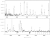 |
Fig. 12 FIES spectrum of 17hx 762 days after discovery (uncorrected for reddening). The Y -axis units are in erg cm−2 s−1 Å−1. |
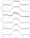 |
Fig. 13 Comparison of the coronal, permitted, and nebular line profiles in the July 2019 FIES spectrum. The profiles share structures and width (see text for details). We plot in gray the same profiles in the May 2019 FIES spectrum, showing invariance of the line profile evolution. The Y -axes are flux in units of erg cm−2 s−1 Å−1. |
7.2 Late spectral appearance and the coronal lines
ASASSN-17hx is also peculiar for the relative strength of its coronal lines. When compared to classical novae followed until their coronal phase as in the CTIO survey by Williams et al. (1991, 1994), we note the following. First, CNe6 that display coronal emissions are well into late nebular phase, with [O III] and [N II] (typically much stronger than Hβ) being the dominant emission lines. Second, the lines of [Fe VII] or higher transitions are always weak compared to both nebular and permitted transitions, usually ≤0.2 I(Hβ). Examples inthe CTIO survey are nova Sco 1989b, nova Sct 1989, nova Cen 1991, nova Oph 1991a, nova LMC 1991, nova Sgr 1991 and nova Pup 1991 (Williams et al. 1991, 1994), and nova Aql 1999b (Iijima & Esenoglu 2003). The only objects that are similar to 17hx are nova Oph 1988 (V2214 Oph) in the CTIO survey, and V723 Cas, that was monitored by Iijima (2006) over 6 yr. Both objects, like 17hx, developed strong coronal lines and weak [O III]. They also displayed strong [Ne V] lines, while for 17hx we lack such information as our spectra are not sufficiently extended in the blue. Both V2214 Oph and V723 Cas were slow novae with extreme oscillations during the early decline (whatever “early” might mean in this case). Strope et al. (2010) classified the first as an S-type nova (i.e., smooth light curve), but they missed early decline data points that are published in Williams et al. (2003, although they lack error bar). V723 Cas, whose light curve Strope et al. (2010) assigned to the J class, had a remarkably slow spectroscopic evolution (Iijima 2006) that is very similar to 17hx. It took about 18 months to enter the optically thin phase. Two years after outburst it showed substantial spectroscopic evolution with dramatic strengthening of the He II line λ4686 and the appearance of the coronal lines from [Fe VI], [Fe VII], and [Ca V], while [O III] remained much weaker than Hβ (Iijima 2006). The ionization of the ejecta further increased, showing [Fe X] over four years after outburst (Iijima 2006). In addition, Iijima (2006) reports broader line profiles in the higher ionization potential transitions (He I and H) than those with low ionization potentials (e.g., Fe II) and similarly more extended wings of the coronal transition relative to the nebular lines in the late spectra. This matches the ionization structure observed in 17hx and is consistent with the ionization structure expected in a ballistically expanding gas powered by a central source.
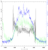 |
Fig. 14 [O III] emission lines (July 2019 FIES spectrum) and the corresponding electron density in velocity space. Shown are [O III]λ5007 (solid blue) and [O III]λ4363 (dotted green). Their units are in erg s−1 cm−2 Å−1, and are indicated in blue on the right axis. The black solid line is the corresponding electron density, ne, per resolution element (units in cm−3 on the left axis). The ne is plotted only within the velocity range [−600,+600] km s−1, beyond which the noise dominates. |
7.3 Ejecta mass
To continue the comparison of 17hx and V723 Cas we look at their ejecta masses. Iijima (2006) used integrated line fluxes to derive an unusually large ne, but a quite low mass (5 × 10⁻⁶ M⊙), possibly incompatible with the observed slow evolution. The line fluxes reported in Iijima’s Table 7 indicate a strongly collisionally damped [O III] ratio four years after outburst. We derived an independent value for the V723 Cas ejecta parameters, estimating the [O III] and Hβ lines intensity from Iijima’s Fig. 14 and modeling their profiles with our Monte Carlo simulation and maximum expansion velocity vmax=1600 km s−1. The upper limit for the mass, for a filling factor of unity, is 0.03 M⊙. Adopting the Schaefer (2018) distance of 5.6 kpc, we derive ε = 0.01 and Mej = 3 × 10⁻⁴ M⊙ for V723 Cas. Although uncertain, these values are similar to those derived for 17hx. The two objects have a somewhat large ejecta mass, about an order of magnitude higher than typical CNe, and possibly more. The largest uncertainty is in the distance: the closer the object, the more CNe-like the ejecta mass, but the smaller the filling factor which falls in the range for recurrent novae (e.g., T Pyx; Shore 2013b). It is interesting to note that these high ejecta masses expand with velocities that are comparable to those of typical CNe, implying larger kinetic energy.
In their nova sequences, Yaron et al. (2005) found an increase in the ejected mass with decreasing white dwarf mass, with a 0.4 M⊙ WD ejecting <7 × 10⁻⁴ M⊙. This is at the lower limit of our range for the ejecta mass in 17hx. Furthermore, since these were one-dimensional simulations, the filling factor is unity by definition. Hence, the mass and kinetic energies we derive are likely far higher than these models produced. The same holds for the TNR results from Starrfield et al. (2013), who found that even for low mass accretion rates and low-mass WDs there is a TNR that can ultimately eject some mass, although neither as much as in Yaron et al. (2005) nor near our estimated value for 17hx. Starrfield et al. (2013) also note that unsteady nuclear burning would result for accretion of solar composition material and no mixing.
7.4 Progenitor
Saito et al. (2017) identified the 17hx progenitor with a Ks ~ 16.7 mag star in the VVVX survey, also matching a nearby Gaia DR2 source of G = 19.3 mag. The Gaia source, once dereddened and scaled to 7.6 kpc (see also Evans et al. 2018), has an absolute magnitude MV ~ 3 mag, consistent with old nova absolute magnitudes determined by Selvelli & Glimozzi (2019). The same exercise repeated in K band produces MK = 2 mag, which is somewhat bright for a cool main sequence companion, but compatible with an evolved donor. Saito’s identification implies that the 17hx outburst amplitude was 11 mag. We note that there are no other visible objects nearby 17hx, and that its outburst amplitude would be much larger than 11 mag should the identification not be confirmed. In contrast, the Gaia DR2 magnitudes and Schaefer’s distance for V723 Cas indicate an absolute magnitude MV ≲ 0.1 mag which does not match an ordinary old nova or quiescent cataclysmic variable.
In conclusion, after this long presentation and physical dissection of the source properties using every tool we have developed for the study of CNe, we cannot be confident about the transient progenitor. Although ASASSN-17hx has many of the earmarks of a classical nova, we may be dealing with an impostor.
Acknowledgements
E.M. deeply thanks John Telting at the NOT telescope for his prompt help, suggestions and exhaustive explanations. The authors are grateful to the people of the ARAS association for making freely available the spectra of their observations. In particular the authors thanks observers Umberto Sollecchia, Lorenzo Franco, Olivier Garde, Tim Lester and Joan Guarro Flo whose data has been displayed in the present paper. We thank the observers registered to the AAVSO database who contributed to the photometric monitoring of ASASSN-17hx. We also thank Kim Page for the help with the XRT data reduction and acknowledge Swift PI and operation staff for approving and planning the Swift observations. P.K. acknowledges support by the UK Space Agency. We also thank the referee, Nye Evans, for his precious feedback.
Appendix A Tables
Epoch of the VLT/UVES observations and the adopted instrument setups.
Log of observations for the transition stage spectra.
Epoch and instrument setup for the NOT/FIES observations.
Swift UV photometry.
References
- Berardi, P., Sims, W., & Sollecchia, U. 2017, ATel 10558 [Google Scholar]
- Bohlin, R. C., Savage, B. D., & Drake, J. F., 1978, ApJ, 224, 132 [NASA ADS] [CrossRef] [Google Scholar]
- Cao, Y., Kasliwal, M. M., Neill, J. D., et al. 2012, ApJ, 752, 133 [NASA ADS] [CrossRef] [Google Scholar]
- De Gennaro Aquino, I., Shore, S. N., Schwarz, G., et al. 2014, A&A, 562, A28 [NASA ADS] [CrossRef] [EDP Sciences] [Google Scholar]
- Dekker, H., D’Odorico, S., & Kaufer, A. 2000, SPIE, 4008, 534 [Google Scholar]
- Duerbeck, H. W. 1981, PASP, 93, 165 [NASA ADS] [CrossRef] [Google Scholar]
- Evans, D. W., Riello, M., De Angeli, F., et al. 2018, A&A, 616, A4 [NASA ADS] [CrossRef] [EDP Sciences] [Google Scholar]
- Frandsen, S., & Lindberg, B. 1999, Anot. Conf, 71 [Google Scholar]
- Guarro, J., Berardi, P., Sollecchia, U., et al. 2017, ATel 10737 [Google Scholar]
- Iliadis, C. 2007, Nuclear Physics of Stars (Wenheim: Wiley-VCH Verlag) [CrossRef] [Google Scholar]
- Iijima, T. 2006, A&A, 451, 563 [NASA ADS] [CrossRef] [EDP Sciences] [Google Scholar]
- Iijima, T., & Esenoglu, H. H. 2003, A&A, 404, 997 [NASA ADS] [CrossRef] [EDP Sciences] [Google Scholar]
- José, J. 2016, Stellar Explosions - Hydrodynamics and Nucleosynthesis (Boca Raton: CRC Press) [Google Scholar]
- Kafka, S. 2019, Observations from the AAVSO International Database, https://www.aavso.org [Google Scholar]
- Kalberla, P. M. W., Burton, W. B., & Hartmann, D., et al. 2005, A&A, 440, 775 [NASA ADS] [CrossRef] [EDP Sciences] [Google Scholar]
- Keenan. P. C., & Hynek, J. A. 1950, ApJ, 111, 1 [NASA ADS] [CrossRef] [Google Scholar]
- Kuin, N. P. M., Page, K. L., Williams, S. C., et al. 2017, ATel, 10636 [Google Scholar]
- Kurtenkov, A. T., Tomov, T., & Pessev, P. 2017a, ATel, 10527 [Google Scholar]
- Kurtenkov, A. T., Napetova, M. & Tomov, T. 2017b, ATel, 10725 [Google Scholar]
- Mason, E., Shore, S. N., De Gennaro Aquino, I., et al. 2018, ApJ, 853, 27 [NASA ADS] [CrossRef] [Google Scholar]
- McLaughlin, D. B. 1943, Publ. Obs. Univ. of Michigan, 8, 149 [NASA ADS] [Google Scholar]
- Munari, U., & Zwitter, T. 1997, A&A, 318, 269 [NASA ADS] [Google Scholar]
- Munari, U., Ochner, P., Hambsch, F. J., et al. 2017a, ATel, 10572 [Google Scholar]
- Munari, U., Traven, G., Hambsch, F.-J., et al. 2017b, ATel, 10641 [Google Scholar]
- Munari, U., Hambsch, F.-J., Frigo, A., et al. 2017c, ATel, 10736 [Google Scholar]
- Osterbrock, D. E., 1989, Astrophysics of Gaseous Nebulae and Active Galactic Nuclei (Mill Valley, CA: University Science Books) [CrossRef] [Google Scholar]
- Pavana, M., Anupama, G. C., Selvakumar, G., & Kiran, B. S. 2017, ATel, 10613 [Google Scholar]
- Payne-Gaposchkin, C. 1957, The Galactic Novae (Amsterdam: North Holland Publishing Company) [Google Scholar]
- Saito, R. K., Hempel, M., & Minniti, D. 2017, ATel, 10552 [Google Scholar]
- Schaefer, B. E. 2018, MNRAS, 481, 3033 [NASA ADS] [CrossRef] [Google Scholar]
- Schlafly, E. F., & Finkbeiner, D. P. 2011, ApJ, 737, 103 [NASA ADS] [CrossRef] [Google Scholar]
- Schwarz, G. J., Ness, J-U., Osborne, J. P., et al. 2011, ApJS, 197, 31 [NASA ADS] [CrossRef] [Google Scholar]
- Schwarzschild, M., & Harm, R. 1965, ApJ, 142, 855 [NASA ADS] [CrossRef] [Google Scholar]
- Selvelli, P., & Gilmozzi, R. 2019, A&A, 622, A186 [NASA ADS] [CrossRef] [EDP Sciences] [Google Scholar]
- Shore, S. N., Sonneborn, G., Starrfield, S., Gonzalez-Riestra, R., & Polidan, R. S. 1994, ApJ, 421, 344 [NASA ADS] [CrossRef] [Google Scholar]
- Shore, S. N., Augusteijn, T., Ederoclite, A., & Uthas, H. 2012, A&A, 537, A2 [NASA ADS] [CrossRef] [EDP Sciences] [Google Scholar]
- Shore, S. N., De Gennaro Aquino, I., Schwarz, G. J., et al. 2013a, A&A, 553, A123 [NASA ADS] [CrossRef] [EDP Sciences] [Google Scholar]
- Shore, S. N., Schwarz, G. J., De Gennaro Aquino, I. et al., 2013b, A&A, 549, A140 [NASA ADS] [CrossRef] [EDP Sciences] [Google Scholar]
- Shore, S. N., Mason, E., Schwarz, G. J. et al., 2016, A&A, 590, A123 [NASA ADS] [CrossRef] [EDP Sciences] [Google Scholar]
- Shore, S. N., Kuin, N. P., Mason, E., & De Gennaro Aquino, I. 2018, A&A, 619, A104 [NASA ADS] [CrossRef] [EDP Sciences] [Google Scholar]
- Stanek, K. Z., Kochanek, C. S., Chomiuk, L., et al. 2017, ATel, 10523 [Google Scholar]
- Starrfield, S., Timmes, F. X., Hix, W. R., et al. 2013, Binary Paths to Type Ia Supernovae Explosions, IAUS (Cambridge: Cambridge University Press), 281, 166 [NASA ADS] [Google Scholar]
- Strope, R. J., Schaefer, B. E., & Henden, A. A. 2010, ApJ, 140, 34 [Google Scholar]
- Telting, J. H., Avila, G., Buchhave, L., et al. 2014, Astron. Nachr., 335, 41 [NASA ADS] [CrossRef] [Google Scholar]
- Williams, S. C., & Darnley, M. J. 2017, ATel, 10542 [Google Scholar]
- Williams, R. E., Hamuy, M., Phillips, M. M., et al. 1991, ApJ, 376, 721 [NASA ADS] [CrossRef] [Google Scholar]
- Williams, R. E., Phillips, M. M., & Hamuy, M. 1994, ApJS, 90, 297 [NASA ADS] [CrossRef] [Google Scholar]
- Williams, R. E., Hamuy, M., Phillips, M. M., et al. 2003, JAD, 9 [Google Scholar]
- Yaron, O., Prialnik, D., Shara, M. M., & Kovetz, A. 2005, ApJ, 623, 410 [Google Scholar]
Astronomical Ring for Access to Spectroscopy: http://www.astrosurf.com/aras/
Many of the ARAS high-resolution spectra are limited to the Hα region.
The relative intensity of the [Ar III] to [Ar V] transitions cannot be compared because they lie in the region of scattered light.
For example, for Swift XRT spectra, the hardness ratio is usually estimated in the interval 0.2–1.0 keV, while our upper cutoff is at the lowest energy end of this band.
For the obvious reasons of the interaction between the ejecta with the donor’s wind, symbiotic novae are excluded from this comparison.
All Tables
All Figures
|
Fig. 1 Top panel: AAVSO V light curve together with the epoch of the UVES observations (blue lines), the ARAS high-resolution un-calibrated and low-resolution flux calibrated spectra (green dotted and solidlines, respectively), the LISA and HEROS observations (red lines), and the FIES spectra (cyan lines). Middle panel: AAVSO B, R, and I light curves together with Swift UVOT UVW1 (λc =2600 Å), UVM2 (λc=2246 Å), and UVW2 (λc1928 Å). Bottom panel: color light curve: (B–V), (V –R), and (V –I). Error bars ≥0.2 mag in the color light curves were arbitrarily set whenever either the V or the paired broadband photometry did not have an associated error bar. Colors were computed every time the V and broadband filter were taken within 3 h observations. |
| In the text | |
|
Fig. 2 Comparison of the temperature profile of the H I 21 cm (red line) with the Na I (black solid line) and Ca II K (black dashed line) interstellar absorption profiles. The two vertical blue dotted lines mark the limits for the column density calculation (see Sect. 2 for details). Units of flux (erg s−1 cm−2 Å−1) and temperature (K) are on the left and right axis, respectively. |
| In the text | |
|
Fig. 3 Four high-resolution spectra taken at VLT/UVES. The spectra have been split in three panels where there is the wavelength gap induced by the dichroic or the detector mosaic (red arm only). Photometric state and age since discovery (in days) are color-coded in the upper panel. The Hα line is saturated in all UVES spectra. The spectra in the figure have not been corrected for reddening. |
| In the text | |
|
Fig. 4 Evolution of the Fe II λ5169 (RMT 42) transition. Y -axis units are in erg cm−2 s−1 Å−1. The blue and red dotted lines indicate the velocity of the persistent narrow absorption (see Sect 4.1) and of the He I absorption in the first UVES spectrum, respectively, for a comparison (see text for details). The photometric state (min, max) of each spectrum is indicated within each panel. |
| In the text | |
|
Fig. 5 Evolution of the Ca I and Ca II line profiles (see text for details). The emission centered at about +500 km s−1 in the first column (Ca I panels) is from Fe II RMT 27. The arrow in the third panel from the top indicates the second broad absorption from Ca I λ4226. The Y -axis units are in erg cm−2 s−1 Å−1. The blue and red dotted lines indicate the velocity of the persistent narrow absorption (see Sect. 4.1) and of the He I absorption in the first UVES spectrum, respectively. The photometric state (min, max) of the spectra is indicated on the left of each row. |
| In the text | |
|
Fig. 6 Evolution of the He I (triplet and singlet) transitions (see text for details). The Y-axis units are in erg cm−2 s−1 Å−1. The reddotted line indicates the velocity of the absorption component at the first epoch: ~1050 km/s. The photometric state (min max) is indicated on the left of each row. |
| In the text | |
|
Fig. 7 Evolution of the Si II doublet (RMT 2) transition (see text for details). The Y-axis units are in erg cm−2 s−1 Å−1. The colored vertical lines are identical to those in the previous figures. The photometric state (min, max) of the spectra is indicated within each panel. |
| In the text | |
|
Fig. 8 Evolution of the O I triplets (RMT 1, top, and 4, bottom). Triplet (1) is resolved in the narrow absorption at approximately −460 km s−1. Together with triplet (1) we overplot the Hδ profile forcomparison (gray line) (see text for details; the H line has been arbitrarily offset in each subpanel; in the bottom subpanel it has also been scaled by a factor 0.5). The blue line of the Ca II triplet is included in the bottom panel; it shows similar behavior to the O I RMT 4. The Y -axis units are in erg cm−2 s−1 Å−1. The colored vertical dotted lines have the usual meaning. The photometric state (min, max) of each spectrum is indicated in each subpanel. |
| In the text | |
|
Fig. 9 Sequence of low-resolution flux calibrated ARAS spectra, together with their position in the V -band light curve. The Y -axis units are in erg cm−2 s−1 Å−1 and mag on the left and right side, respectively. Each panel plots in gray the previous spectra for easier comparison. |
| In the text | |
|
Fig. 10 Evolution across four min-max cycles of the H, He I, and Fe II lines, representing respectively intermediate, high, and low ionization potential energy atoms. The exact photometric state of each spectrum is indicated in the panels of the first column; the age (in days) is on the left. The He I transition is contaminated by Na I D both of interstellar and ejecta origin. The Na I D transition (emission and absorption) originating in the ejecta is particularly evident in the spectra taken between day 82 and 101. |
| In the text | |
|
Fig. 11 LISA (top panel) and HEROS (mid and bottom panels) spectra of 17hx ~1 yr after outburst and/or discovery. The LISA spectrum is in units of erg cm−2 s−1 Å−1 and uncorrected for reddening, while the HEROS spectrum is in arbitrary units. The spectrograph and the age of the spectrum are indicated in each panel. |
| In the text | |
|
Fig. 12 FIES spectrum of 17hx 762 days after discovery (uncorrected for reddening). The Y -axis units are in erg cm−2 s−1 Å−1. |
| In the text | |
|
Fig. 13 Comparison of the coronal, permitted, and nebular line profiles in the July 2019 FIES spectrum. The profiles share structures and width (see text for details). We plot in gray the same profiles in the May 2019 FIES spectrum, showing invariance of the line profile evolution. The Y -axes are flux in units of erg cm−2 s−1 Å−1. |
| In the text | |
|
Fig. 14 [O III] emission lines (July 2019 FIES spectrum) and the corresponding electron density in velocity space. Shown are [O III]λ5007 (solid blue) and [O III]λ4363 (dotted green). Their units are in erg s−1 cm−2 Å−1, and are indicated in blue on the right axis. The black solid line is the corresponding electron density, ne, per resolution element (units in cm−3 on the left axis). The ne is plotted only within the velocity range [−600,+600] km s−1, beyond which the noise dominates. |
| In the text | |
Current usage metrics show cumulative count of Article Views (full-text article views including HTML views, PDF and ePub downloads, according to the available data) and Abstracts Views on Vision4Press platform.
Data correspond to usage on the plateform after 2015. The current usage metrics is available 48-96 hours after online publication and is updated daily on week days.
Initial download of the metrics may take a while.