| Issue |
A&A
Volume 634, February 2020
|
|
|---|---|---|
| Article Number | L9 | |
| Number of page(s) | 7 | |
| Section | Letters to the Editor | |
| DOI | https://doi.org/10.1051/0004-6361/201936608 | |
| Published online | 05 February 2020 | |
Letter to the Editor
Effect of metallicity on the detectability of rotational periods in solar-like stars
1
Max Planck Institute for Solar System Research, Justus-von-Liebig-Weg 3, 37077 Göttingen, Germany
e-mail: This email address is being protected from spambots. You need JavaScript enabled to view it.
2
School of Space Research, Kyung Hee University, Yongin, Gyeonggi, 446-701, Republic of Korea
Received:
30
August
2019
Accepted:
24
December
2019
Abstract
The accurate determination of stellar rotation periods is important for estimating stellar ages and for understanding stellar activity and evolution. While rotation periods can be determined for about thirty thousand stars in the Kepler field, there are over one hundred thousand stars, especially with low photometric variability and irregular pattern of variations, for which rotational periods are unknown. Here we investigate the effect of metallicity on the detectability of rotation periods. This is done by synthesising light curves of hypothetical stars that are identical to our Sun with the exception of the metallicity. These light curves are then used as an input to the period determination algorithms. We find that the success rate for recovering the rotation signal has a minimum close to the solar metallicity value. This can be explained by the compensation effect of facular and spot contributions. In addition, selecting solar-like stars with near-solar effective temperature and photometric variability, and with metallicity between M/H = −0.35 and M/H = 0.35 from the Kepler sample, we analyse the fraction of stars for which rotational periods have been detected as a function of metallicity. In agreement with our theoretical estimate we find a local minimum for the detection fraction close to the solar metallicity. We further report rotation periods of 87 solar-like Kepler stars for the first time.
Key words: stars: variables: general / stars: rotation / stars: fundamental parameters / stars: solar-type
© V. Witzke et al. 2020
 Open Access article, published by EDP Sciences, under the terms of the Creative Commons Attribution License (http://creativecommons.org/licenses/by/4.0), which permits unrestricted use, distribution, and reproduction in any medium, provided the original work is properly cited.
Open Access funding provided by Max Planck Society.
1. Introduction
The rotation period of a star is a fundamental stellar parameter that is closely linked to the stellar age, and determines its magnetic activity. Skumanich (1972) was the first to demonstrate that the equatorial rotational velocity and magnetic activity (the latter expressed via the emission in the Ca II H and K line cores) decrease with stellar age t as  . Thereafter, an age–rotation–activity relation was established that indicates that young stars generally rotate faster and are more active than old stars (Noyes et al. 1984). Hence, determining stellar rotation periods is crucial for assessing the stellar age (Kawaler 1989; Barnes 2003), which otherwise can be measured through asteroseismology, for example.
The rotational signal is imprinted in the stellar photometric variability, which is caused by transits of magnetic features (such as spots and faculae) across the visible disc and by their temporal evolution. With the advent of large photometric surveys, for example the Kepler mission, stellar photometric light curves have been measured for an extensive number of main-sequence stars. This has allowed the determination of rotational periods for about thirty thousand stars (McQuillan et al. 2013a,b; Reinhold et al. 2013; Walkowicz & Basri 2013; Nielsen et al. 2013; McQuillan et al. 2014; do Nascimento et al. 2014; García et al. 2014; Reinhold & Gizon 2015; Ceillier et al. 2016; Buzasi et al. 2016). Among these studies, the largest homogeneous set of rotation periods was derived by McQuillan et al. (2014), who measured rotation periods for 34 030 Kepler stars. Despite this huge number of stars with determined rotation periods, a significant rotation signal could not be detected in an even bigger sample of 99 000 stars (see Table 2 in McQuillan et al. 2014). Stellar samples with known rotation periods form the basis for many studies, ranging from galactic evolution to the solar-stellar connection (Buzasi et al. 2016; Davenport 2017; Davenport & Covey 2018; Reinhold et al. 2019a,b; Notsu et al. 2019; van Saders et al. 2019). Consequently, the conclusions drawn in these studies might be strongly biased towards the behaviour of stars for which rotation periods could be determined.
To investigate potential detectability biases, it is essential to understand possible physical reasons for a lack of the rotational signal in these stars. Our Sun provides a good example of a star whose highly irregular temporal profile of the photometric variability hampers the determination of the rotational period. It has been shown that the irregular profile of solar variability is associated with the cancellation of facular and spot rotational signals in broad-band photometric measurements (Shapiro et al. 2017, 2020; Reinhold et al. 2019a). One can expect that such a cancellation might also apply to other solar-like stars, in particular those with a near-solar level of magnetic activity. This assumption is in line with recent results that the low success rate of less than 20% for the period determination in stars with near-solar effective temperatures (see Fig. 14 in van Saders et al. 2019) cannot be explained by the low signal-to-noise ratio in their photometric records. In addition, Reinhold et al. (2019a) proposed that the cancellation of bright faculae and dark spots leads to a non-detection at intermediate rotation periods in the Kepler field.
It was shown earlier that metallicity has a significant effect on facular contrasts, and thus on stellar variability in solar-like stars (Karoff et al. 2018; Witzke et al. 2018). In this work, our aim is to understand the effect of metallicity on the detectability of the rotation periods in solar-like stars. We employ an extended version of the widely used model of solar brightness variability, the Spectral And Total Irradiance REconstruction (SATIRE; Fligge et al. 2000; Krivova et al. 2003). This model reconstructs stellar brightness variability based on solar magnetograms and disc images. To study the influence of metallicity on the detectability of rotational periods we generate light curves for different metallicities, and calculate the success rates for recovering the rotational signal by using periodograms. Subsequently, we analyse a sample of Kepler stars with near-solar values of effective temperature, photometric variability, and rotation periods, and compare the effect of metallicity on the detectability of rotational periods in observations and the theoretical model.
2. Rotation period detectability in solar-like stars
2.1. Modelling
In this section we study the effect of metallicity on the success rate of determining rotational periods in solar-like stars. We employ the SATIRE (Krivova et al. 2003) model, which attributes stellar variability to the time-dependent contributions from magnetic features on the stellar surface, which can be divided into dark (spots and pores) and bright (faculae and network) features. Recently, this model was generalised for calculating variability of stars with different metallicities (Witzke et al. 2018) by recalculating spectra of the quiet and magnetic stellar regions. Here we follow up this approach and generate light curves in the Kepler filter for stars identical to the Sun in all aspects except metallicity. In particular, we assumed the solar distribution of magnetic features, but recalculated their contrasts as a function of metallicity.
Figure 1 shows example light curves for three different metallicity values obtained by using the solar magnetic feature distributions observed during solar cycle 23, which was a cycle of intermediate strength. Since the time series of magnetic feature distribution is derived from SoHO/MDI observations (Scherrer et al. 1995), the modelled light curves are as seen by an observer on Earth. For M/H = −0.3 (Fig. 1a) the flux decreases during the activity cycle maximum in 2001–2003, indicating a spot-dominated variability on the timescale of the 11-year activity cycle. The opposite is observed for the solar case (Fig. 1b), and a star with M/H = 0.3 (Fig. 1c), where the flux increases during the activity maximum. These three cases demonstrate the transition from spot-dominated to faculae-dominated regimes on the activity cycle timescale.
 |
Fig. 1. Model light curves for different M/H values in the Kepler pass band: (a) M/H = −0.3, (b) solar value, (c) M/H = 0.3. The insets show shorter time intervals to better visualise the rotational variability. |
We measure the photometric variability of a star on the rotational timescale by using the variability range Rvar. This quantity is defined as the difference between the 95th and 5th percentile of the sorted differential intensities in the light curve (Basri et al. 2010, 2011). Table 1 illustrates how the amplitude of Rvar depends on the metallicity. The Rvar values in Table 1 are obtained by splitting the 1998–2011 light curves in subsequent 90-day intervals, and calculating the median of all individual Rvar values for each of the intervals.
Rvar with metallicity.
We find a slight increase in Rvar for M/H = 0.3 (Rvar = 0.074 compared to Rvar = 0.062 for the solar case) and a significant increase for M/H = −0.3, Rvar = 0.125 (see Table 1). This behaviour in Rvar is caused by the effect of metallicity on the balance of spot to facular contrast. It is similar to the effect found in Witzke et al. (2018), but not as pronounced because the variability on the rotation timescale, Rvar, is mainly attributed to spots, whereas the predominant contribution to the variability on the magnetic activity timescale for the Sun comes from faculae. We note that our approach employs 1D atmosphere models, which do not take 3D effects into account. While 3D effects might lead to slightly different quantitative results, the overall trends are nicely captured in 1D.
We investigate whether the detection of the Carrington synodic rotation (i.e. the rotation signal of 27.3 days) is possible for such stars. In order to emulate light curves of Kepler stars, we randomly chose four-year intervals in the generated light curves. As we expect the detectability to depend on the phase of the activity cycle, we aim to capture the full activity cycle 23 (from mid-1996 to the end of 2008). To this end the 500 randomly chosen four-year intervals were restricted to lie between mid-1994 and the end of 2011. The additional two years before and after cycle 23 are needed to obtain a uniform distribution of the positions of the middle point of the four-year intervals within cycle 23. To obtain the recovery rate of the solar rotation period, we applied generalised Lomb-Scargle periodograms (Zechmeister & Kürster 2009) to each realisation of the four-year intervals, and searched for a rotational signal. First, we determined the standard deviation, σ, of the power in the range of 0–50 days in the periodogram. Only if the highest power peak in the periodogram satisfied the following four criteria did we assume it as a successfully recovered rotation period: i) it is the highest peak in the range of 0–50 days, ii) the peak is higher than 5σ, iii) the second highest peak is at least 20% lower, and iv) the rotational period associated with this peak is between 24 and 30 days. Figure 2 shows the recovery rates in percent for different metallicities. It shows that for stars with near-solar metallicity the detection rate is very low. This occurs because of the absence of a significant peak in the periodogram for almost all of the 500 randomly chosen time intervals for such metallicities. The detection rate increases significantly for metallicity values that are about 0.2 dex different from the solar value, reaching more than 55% for M/H = −0.3.
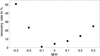 |
Fig. 2. Recovery rates for determining the rotational period in the range of 24–30 days for different metallicities. |
To understand the dependence of the success rates on the metallicity, we investigate the facular and spot components of the light curves separately. The SATIRE model uses decomposed spectral fluxes from quiet regions, facular regions, and spot regions, which enables us to generate separate light curves for the facular and spot components. We studied the contribution of the facular- and spot- components to the rotational signal. For a better illustration we employed global wavelet power spectra instead of periodograms. We considered the time interval of the whole cycle 23, and we calculated the power spectra using Morlet wavelets of the order six. In Fig. 3 the power spectra for the cases with M/H = −0.3, M/H = −0.2, M/H = −0.1, M/H = 0.0 and M/H = 0.3 are shown, where the solar case is included as a reference.
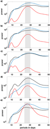 |
Fig. 3. Power spectra of the facular (red), spot (blue), and total (black) components for different metallicities: (a) solar case as reference, (b) M/H = −0.1, (c) M/H = −0.2, (d) M/H = −0.3, (e) M/H = 0.3. The grey area indicates periods of 24–30 days. |
Since we are interested in the solar rotational signal, we focus on the range of 24–30 days. For the solar case (Fig. 3a), the power obtained from the total light curve lies in between the power of the facular and the spot components. Although both the facular- and the spot power spectra show a peak, the contribution of the bright faculae cancels the brightness contribution of the dark spots (Shapiro et al. 2017). Thus, there is no pronounced signal in the total power spectrum on the rotational timescale. Since the success rates above were calculated for 500 different intervals, some of the intervals correspond to the activity minimum, where no or only few spots occur. For such intervals, it is possible to find the rotational signal due to the faculae (Lanza & Shkolnik 2014). The case with M/H = −0.1 has a similarly flat power spectrum around the 24–30 days interval. The power of the total light curve lies in between the power of the facular and the spot components, but the power of the facular component is lower compared to the M/H = 0.0 case. This difference affects the compensation between faculae and spots, and thus can explain the lower success rates for M/H = −0.1 (see Fig. 2).
For the case with M/H = −0.2 the power of the total light curve lies also between the power of the facular and spot component, but the power of the facular component is very small. The decreased power in the faculae results from a smaller facular contrast at the limb, and even a slightly darker faculae at the disc centre (see Fig. B.1). Thus the spot darkening prevails, and a determination of the rotational period becomes possible. Decreasing the metallicity further leads to a significant darkening of faculae at the disc centre (see Fig. B.1). Such that the facular contribution adds onto the spot contribution, which becomes evident from Fig. 3d), where the total component shows a clear peak and is above the facular and the spot components. In contrast to this, at large metallicity values, e.g. M/H = 0.3 facular brightening becomes dominant (see Fig. 3e). This also results in an increased detectability of the rotational period.
2.2. Analysis of Kepler observations
We now investigate whether a similar trend with metallicity can also be found for solar-like Kepler stars. We follow the selection criteria of Reinhold et al. (2019b) to focus on solar-like main-sequence stars. In particular, we select a sample of stars with effective temperatures in the range 5600–5900 K (which corresponds to the solar effective temperature ±150 K), surface gravities log g > 4.2, and metallicities in the range −0.35 < M/H < 0.35. Stars fainter than 15th Kepler magnitude are discarded. Stellar fundamental parameters (Teff, log g, M/H) are adopted from Mathur et al. (2017) based on the latest Kepler data release 25. Reinhold et al. (2019b) further used Gaia DR2 data to construct a Hertzsprung-Russell diagram (HRD), and select only stars confined between two isochrones: the “lower” one with an age of 4 Gyr and metallicity of −0.8 dex, and an “upper” isochrone with an age of 5 Gyr and metallicity of 0.3 dex. Furthermore, we focus on stars with near-solar photometric variability. The solar variability changes over the activity cycle, reaching Rvar values up to 0.18% (Reinhold et al. 2019b). Thus, we restrict our sample to stars with Rvar < 0.18%. These selection criteria yield 911 stars in total.
Figure 4 shows the metallicity distribution in our sample. The distribution has a pronounced peak at around M/H = −0.1. However, the uncertainties are quite large (up to ±0.3 dex). To account for measurement uncertainties in the metallicity values, we describe the stars by a density distribution function, rather than using discrete values. For each star we used a normalised Gaussian distribution function, where the mean is set to the star’s metallicity value and for the standard deviation we take the measurement uncertainty. The sum over all 911 metallicity distribution functions is shown by the red curve in Fig. 4.
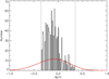 |
Fig. 4. Metallicity distribution of all selected stars. The sample contains 911 stars with Rvar < 0.18%. Black: histogram of stars in the metallicity range −0.35 < M/H < 0.35, which is indicated by the grey lines. Red: The metallicity distribution using normalised Gaussian functions to account for the metallicity measurement uncertainty. |
To investigate a link between metallicity and the detectability of rotational periods, we further distinguish between stars with detected rotational periods (Table 1 in McQuillan et al. 2014), and without a significant period detection (Table 2 in McQuillan et al. 2014). Hereafter, these two samples are referred to as the periodic and the non-periodic samples, respectively. For stars in the periodic sample, we restrict the rotation periods to the range 24–30 days. Unfortunately, McQuillan et al. (2014) found rotation periods for only 10 stars in our sample. This number of stars is not sufficient to get a meaningful metallicity distribution of stars with known rotation periods. Thus, we searched for potentially undetected periods for all stars in Table 2 of McQuillan et al. (2014) which satisfy our selection criteria. Analysing the full 4-yr Kepler time series using Lomb-Scargle periodograms and auto-correlation functions, we were able to derive rotation periods for additional 87 stars (for details see Appendix A and Table A.1). Thus, the above constraints yield 97 stars with determined rotation periods, and 814 stars with unknown rotation period.
Figure 5 shows the detection fraction as a function of metallicity. For that we used the ratio of the metallicity distributions of stars with known rotation periods, nper(M/H), to the total number of stars (with known and unknown rotational periods), nall(M/H). Our null hypothesis is that there is no effect of metallicity on the detection fraction, such that we expect a constant value (97/911), which is indicated by black dots in Fig. 5.
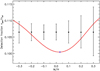 |
Fig. 5. Detection fraction as a function of metallicity (red line). The detection fraction is defined as the ratio of the density distribution of stars with known rotation periods, nper, to the density distribution of the total number of stars, nall. The black dots indicate the expected ratio, which is derived as the ratio of all periodic stars to all stars in a sample. The error bars correspond to the standard deviation using 10 000 realisations by randomly choosing 97 stars. The blue star indices the minimum of the detection fraction. |
We evaluated the statistical significance of the calculated detection fractions at seven metallicity values. For that, we randomly chose 97 stars from the total sample. We repeated this 10 000 times, and calculated the mean value of the detection fraction at seven metallicity values between M/H = −0.3 and M/H = 0.3. The mean values are identical with the expected ratio. Subsequently, the standard deviation from the expected ratio is obtained from the 10 000 realisations, and indicated by the error bars.
Remarkably, solar-like stars in the Kepler sample show a similar trend as found for the generated light curves for different metallicities (see Sect. 2.1). The detection fraction shows a minimum around solar metallicity, and increases towards lower and higher metallicities. In the range −0.15 < M/H < 0.15 the obtained fractions are below the standard deviation, i.e. significant. At the same time, M/H < −0.15 and M/H > 0.15 the detection fractions remain within the error bars due to large metallicity uncertainties and low number statistics.
3. Conclusions
The Kepler field of view was selected in order to contain a large fraction of solar-like stars. Focusing on stars in the effective temperature range of 5600 K–5900 K, it is challenging to determine their rotational periods (see Fig. 14 in van Saders et al. 2019). Moreover, Reinhold et al. (2019b) show that the majority of the solar-like stars for which rotational periods could not be determined exhibit near-solar photometric variability, Rvar. Here, we have provided one possible explanation for a decreased detection fraction for these stars.
We investigated the compensation of the facular and spot contributions to the rotational signal in stellar photometric light curves. This compensation hampers the detection of stellar rotational periods, and contributes to a decreased detection rate for solar-like stars. Our results show that the detectability of rotational periods in stars with solar-like photometric variability crucially depends on metallicity. Hence, metallicity is one additional important parameter to consider when investigating solar-like stars, and more accurate measurements of metallicity are needed.
Acknowledgments
This work has received funding from the European Research Council (ERC) under the European Union’s Horizon 2020 research and innovation programme (grant agreement No. 715947). This work has been partially supported by the BK21 plus programme through the National Research Foundation (NRF) funded by the Ministry of Education of Korea. We would like to thank the International Space Science Institute, Bern, for their support of science team 446 and the resulting helpful discussions. We would like to thank Jennifer van Saders for helpful discussion.
References
- Barnes, S. A. 2003, ApJ, 586, 464 [NASA ADS] [CrossRef] [Google Scholar]
- Basri, G., Walkowicz, L. M., Batalha, N., et al. 2010, ApJ, 713, L155 [NASA ADS] [CrossRef] [Google Scholar]
- Basri, G., Walkowicz, L. M., Batalha, N., et al. 2011, AJ, 141, 20 [NASA ADS] [CrossRef] [Google Scholar]
- Buzasi, D., Lezcano, A., & Preston, H. L. 2016, J. Space Weather Space Clim., 6, A38 [Google Scholar]
- Ceillier, T., van Saders, J., García, R. A., et al. 2016, MNRAS, 456, 119 [NASA ADS] [CrossRef] [Google Scholar]
- Davenport, J. R. A. 2017, ApJ, 835, 16 [CrossRef] [Google Scholar]
- Davenport, J. R. A., & Covey, K. R. 2018, ApJ, 868, 151 [NASA ADS] [CrossRef] [Google Scholar]
- do Nascimento, Jr., J.-D., García, R. A., Mathur, S., et al. 2014, ApJ, 790, L23 [NASA ADS] [CrossRef] [Google Scholar]
- Fligge, M., Solanki, S. K., & Unruh, Y. C. 2000, A&A, 353, 380 [NASA ADS] [Google Scholar]
- García, R. A., Ceillier, T., Salabert, D., et al. 2014, A&A, 572, A34 [NASA ADS] [CrossRef] [EDP Sciences] [Google Scholar]
- Karoff, C., Metcalfe, T. S., Ângela, R. G. S., et al. 2018, ApJ, 852, 46 [NASA ADS] [CrossRef] [Google Scholar]
- Kawaler, S. D. 1989, ApJ, 343, L65 [NASA ADS] [CrossRef] [Google Scholar]
- Krivova, N. A., Solanki, S. K., Fligge, M., & Unruh, Y. C. 2003, A&A, 399, L1 [NASA ADS] [CrossRef] [EDP Sciences] [Google Scholar]
- Lanza, A. F., & Shkolnik, E. L. 2014, MNRAS, 443, 1451 [NASA ADS] [CrossRef] [Google Scholar]
- Mathur, S., Huber, D., Batalha, N. M., et al. 2017, ApJS, 229, 30 [NASA ADS] [CrossRef] [Google Scholar]
- McQuillan, A., Aigrain, S., & Mazeh, T. 2013a, MNRAS, 432, 1203 [NASA ADS] [CrossRef] [MathSciNet] [Google Scholar]
- McQuillan, A., Mazeh, T., & Aigrain, S. 2013b, ApJ, 775, L11 [Google Scholar]
- McQuillan, A., Mazeh, T., & Aigrain, S. 2014, ApJS, 211, 24 [NASA ADS] [CrossRef] [MathSciNet] [Google Scholar]
- Nielsen, M. B., Gizon, L., Schunker, H., & Karoff, C. 2013, A&A, 557, L10 [NASA ADS] [CrossRef] [EDP Sciences] [Google Scholar]
- Notsu, Y., Maehara, H., Honda, S., et al. 2019, ApJ, 876, 58 [NASA ADS] [CrossRef] [Google Scholar]
- Noyes, R. W., Hartmann, L. W., Baliunas, S. L., Duncan, D. K., & Vaughan, A. H. 1984, ApJ, 279, 763 [NASA ADS] [CrossRef] [Google Scholar]
- Reinhold, T., & Gizon, L. 2015, A&A, 583, A65 [NASA ADS] [CrossRef] [EDP Sciences] [Google Scholar]
- Reinhold, T., Reiners, A., & Basri, G. 2013, A&A, 560, A4 [NASA ADS] [CrossRef] [EDP Sciences] [Google Scholar]
- Reinhold, T., Bell, K. J., Kuszlewicz, J., Hekker, S., & Shapiro, A. I. 2019a, A&A, 621, A21 [NASA ADS] [CrossRef] [EDP Sciences] [Google Scholar]
- Reinhold, T., Shapiro, A. I., Solanki, S. K., et al. 2019b, Science, submitted [Google Scholar]
- Scherrer, P. H., Bogart, R. S., Bush, R. I., et al. 1995, Sol. Phys., 162, 129 [Google Scholar]
- Shapiro, A. I., Amazo-Gómez, E., Krivova, N. A., & Solanki, S. K. 2020, A&A, 633, A32 [NASA ADS] [CrossRef] [EDP Sciences] [Google Scholar]
- Shapiro, A. I., Solanki, S. K., Krivova, N. A., et al. 2017, Nat. Astron., 1, 612 [NASA ADS] [CrossRef] [Google Scholar]
- Skumanich, A. 1972, ApJ, 171, 565 [NASA ADS] [CrossRef] [Google Scholar]
- van Saders, J. L., Pinsonneault, M. H., & Barbieri, M. 2019, ApJ, 872, 128 [NASA ADS] [CrossRef] [Google Scholar]
- Walkowicz, L. M., & Basri, G. S. 2013, MNRAS, 436, 1883 [NASA ADS] [CrossRef] [Google Scholar]
- Witzke, V., Shapiro, A. I., Solanki, S. K., Krivova, N. A., & Schmutz, W. 2018, A&A, 619, A146 [NASA ADS] [CrossRef] [EDP Sciences] [Google Scholar]
- Zechmeister, M., & Kürster, M. 2009, A&A, 496, 577 [NASA ADS] [CrossRef] [EDP Sciences] [Google Scholar]
Appendix A: Kepler rotation periods
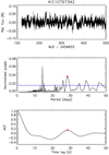 |
Fig. A.1. Period detection for the star KIC 10797342. Top panel: part of the full 4 yr light curve showing photometric variability. Middle panel: Lomb-Scargle periodogram showing several peaks above the 5σ threshold (blue line). Bottom panel: auto-correlation function showing one pronounced peak indicated by the red asterisk. |
Stellar fundamental parameters and rotation periods of the 97 periodic stars in our sample.
We analysed stars from Table 2 in McQuillan et al. (2014) satisfying our selection criteria (i.e. the non-periodic sample) to search for potentially undetected rotation periods. The Kepler data used in this study were reduced with the Presearch Data Conditioning (PDC) pipeline (version 8.0-9.2). We appended all available Kepler quarters by dividing each light curve by its median and subtracting unity. Then we rebinned the data from 30-minute to 6-hour cadences, and analysed the full 4-year time series using Lomb-Scargle periodograms and auto-correlation functions. The Lomb-Scargle periodogram return peaks of different power on a period grid. The peak height is equivalent to the goodness of sine fit to the data, i.e. the more sinusoidal the signal, the higher the peak at this period. At the same time, the auto-correlation function (ACF) searches for self-similarity of the light curve signal, independently of the shape of the signal, and returns a peak at the best time lag (i.e. the ACF period). Since the time series of these slowly rotating solar-like stars are usually non-sinusoidal, we use the ACF period as initial period guess. For both the periodogram and the ACF, we searched for cases where both methods returned consistent peaks, with periods of up to 50 days. The term “consistent” covers different cases. In case a) the periodogram and the ACF both show a pronounced peak at roughly the same period (i.e. the periods may differ by up to five days). This case is considered the easiest one, and we do not show an example here. In case b) the ACF shows a pronounced peak and the periodogram also shows a peak at this period, which still lies above the 5σ threshold (blue line). The highest periodogram peak lies at the half period (i.e. the first harmonic of the rotation period). This case is shown in Fig. A.1, and for this star we report a rotation period Prot = 28.3 days. In case c) the ACF shows a peak, and the periodogram shows many peaks of different height close to the ACF period. The outer envelope of these peaks has a shape similar to that of the ACF peak. The various cases described above show that it is non-trivial to assign a significance to a certain peak. As an additional test, each light curve was inspected by eye to search for the detected periodicity. Cases where it was not clear whether the detected period is the correct rotation period or only the half period (i.e. the first harmonic) were discarded. We distinguish three different cases for a non-detection. The first is when no peak above the 5σ threshold is detected. The second is when the periodogram shows several peaks of the same height, and it is not clear which of them is the correct rotation period. The third case is when the periodogram shows a significant peak, while the ACF shows no peak or a peak at a period that is not a harmonic of the peak detected by the periodogram.
Appendix B: Centre-to-limb variation
To investigate the behaviour of the power spectrum for the facular contribution we calculate the centre-to-limb variation, CLV, for the facular contrast. The facular power spectra for different metallicity show pronounced harmonics of differing strengths (see Fig. 3). The strength of the harmonic is affected by the shape of the light curve caused by a single faculae transiting, and thus depends on the centre-to-limb variations of facular brightness.
Figure B.1 shows the CLV of the facular contrast in the Kepler pass band for the solar case, and the three different metallicity values M/H = {−0.3, −0.2, 0.3}. Most cases correspond to the considered cases in Sect. 2.1. The facular contrast is multiplied by the corresponding μ, which is the cosine of the angle between the observer’s direction and the local stellar radius, to account for the foreshortening effect.
For the solar case, the facular contrast increases from the disc centre outwards. This increase continues almost to the edge of the disc, before it drops again. Such a CLV will result in a doubled peaked feature transition curve, which leads to several pronounced harmonics in the power spectrum (see Fig. 3a). While for a feature transition all harmonics are present in the power spectra, which of them are more pronounced will depend on the shape of the feature transition curve. For a more detailed discussion, see Shapiro et al. (2020).
On the contrary, for the case with higher metallicity (M/H = 0.3), the facular contrast in the middle of the disc is almost constant, while a steep drop starts at r/R ≈ 0.7. This results in an almost smooth peak in the feature transition curve, and thus less pronounced harmonics (see Fig. 3e). For the cases with M/H = −0.2 and −0.3, a similar dip in the contrast appears at the edge and disc centre as in the solar case, which also leads to a double peaked feature transition curve. In addition, the contrast becomes negative towards the disc centre. The faculae are only brighter at the limb, but become dark at the disc centre.
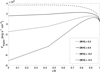 |
Fig. B.1. Centre-to-limb variation of facular flux difference. Here r/R is the normalised radial distance from the centre of the stellar disc. Flux differences for different metallicities are shown in the Kepler pass band. |
All Tables
Stellar fundamental parameters and rotation periods of the 97 periodic stars in our sample.
All Figures
|
Fig. 1. Model light curves for different M/H values in the Kepler pass band: (a) M/H = −0.3, (b) solar value, (c) M/H = 0.3. The insets show shorter time intervals to better visualise the rotational variability. |
| In the text | |
|
Fig. 2. Recovery rates for determining the rotational period in the range of 24–30 days for different metallicities. |
| In the text | |
|
Fig. 3. Power spectra of the facular (red), spot (blue), and total (black) components for different metallicities: (a) solar case as reference, (b) M/H = −0.1, (c) M/H = −0.2, (d) M/H = −0.3, (e) M/H = 0.3. The grey area indicates periods of 24–30 days. |
| In the text | |
|
Fig. 4. Metallicity distribution of all selected stars. The sample contains 911 stars with Rvar < 0.18%. Black: histogram of stars in the metallicity range −0.35 < M/H < 0.35, which is indicated by the grey lines. Red: The metallicity distribution using normalised Gaussian functions to account for the metallicity measurement uncertainty. |
| In the text | |
|
Fig. 5. Detection fraction as a function of metallicity (red line). The detection fraction is defined as the ratio of the density distribution of stars with known rotation periods, nper, to the density distribution of the total number of stars, nall. The black dots indicate the expected ratio, which is derived as the ratio of all periodic stars to all stars in a sample. The error bars correspond to the standard deviation using 10 000 realisations by randomly choosing 97 stars. The blue star indices the minimum of the detection fraction. |
| In the text | |
|
Fig. A.1. Period detection for the star KIC 10797342. Top panel: part of the full 4 yr light curve showing photometric variability. Middle panel: Lomb-Scargle periodogram showing several peaks above the 5σ threshold (blue line). Bottom panel: auto-correlation function showing one pronounced peak indicated by the red asterisk. |
| In the text | |
|
Fig. B.1. Centre-to-limb variation of facular flux difference. Here r/R is the normalised radial distance from the centre of the stellar disc. Flux differences for different metallicities are shown in the Kepler pass band. |
| In the text | |
Current usage metrics show cumulative count of Article Views (full-text article views including HTML views, PDF and ePub downloads, according to the available data) and Abstracts Views on Vision4Press platform.
Data correspond to usage on the plateform after 2015. The current usage metrics is available 48-96 hours after online publication and is updated daily on week days.
Initial download of the metrics may take a while.