| Issue |
A&A
Volume 634, February 2020
|
|
|---|---|---|
| Article Number | A114 | |
| Number of page(s) | 29 | |
| Section | Extragalactic astronomy | |
| DOI | https://doi.org/10.1051/0004-6361/201936321 | |
| Published online | 19 February 2020 | |
LLAMA: The MBH–σ⋆ relation of the most luminous local AGNs
1
Leiden Observatory, PO Box 9513, 2300 RA Leiden, The Netherlands
e-mail: This email address is being protected from spambots. You need JavaScript enabled to view it.
2
Instituto de Astrofísica e Ciências do Espaço, Universidade do Porto, CAUP, Rua das Estrelas, 4150-762 Porto, Portugal
3
Max-Planck-Institut für Extraterrestrische Physik, Postfach 1312, 85741 Garching, Germany
4
Department of Physics & Astronomy, University of Alaska Anchorage, Anchorage, AK 99508-4664, USA
5
Eureka Scientific Inc, Oakland, CA, USA
6
Institute of Astronomy and Astrophysics, Academia Sinica, 11F of AS/NTU Astronomy-Mathematics Building, No.1, Sec. 4, Roosevelt Rd, Taipei 10617, Taiwan
7
Astrophysics Research Institute, Liverpool John Moores University, IC2 Liverpool Science Park, 146 Brownlow Hill, Liverpool L3 5RF, UK
8
Center for Astrophysics and Space Astronomy, University of Colorado, Boulder, CO 80309-0389, USA
9
Universidade Federal de Santa Maria, Departamento de Física/CCNE, 97105-900 Santa Maria, RS, Brazil
10
Departamento de Astronomia, Universidade Federal do Rio Grande do Sul, IF, CP 15051, 91501-970 Porto Alegre, RS, Brazil
11
Centre for Extragalactic Astronomy, Department of Physics, Durham University, South Road, Durham DH1 3LE, UK
12
Universitäts-Sternwarte München, Scheinerstraße 1, 81679 München, Germany
13
Harvard-Smithsonian Center for Astrophysics, 60 Garden St., Cambridge, MA 02138, USA
14
Department of Astronomy and Joint Space-Science Institute, University of Maryland, College Park, Maryland 20742, USA
15
Institute of Astronomy and Kavli Institute for Cosmology Cambridge, University of Cambridge, Cambridge CB3 0HA, UK
16
Space Sciences, Technologies, and Astrophysics Research Institute, Université de Liège, 4000 Sart Tilman, Belgium
17
Department of Physics, California Polytechnic State University, San Luis Obispo, CA 93407, USA
Received:
15
July
2019
Accepted:
13
December
2019
Abstract
Context. The MBH–σ⋆ relation is considered a result of coevolution between the host galaxies and their supermassive black holes. For elliptical bulge hosting inactive galaxies, this relation is well established, but there is still discussion concerning whether active galaxies follow the same relation.
Aims. In this paper, we estimate black hole masses for a sample of 19 local luminous active galactic nuclei (AGNs; LLAMA) to test their location on the MBH–σ⋆ relation. In addition, we test how robustly we can determine the stellar velocity dispersion in the presence of an AGN continuum and AGN emission lines, and as a function of signal-to-noise ratio.
Methods. Supermassive black hole masses (MBH) were derived from the broad-line-based relations for Hα, Hβ, and Paβ emission line profiles for Type 1 AGNs. We compared the bulge stellar velocity dispersion (σ⋆) as determined from the Ca II triplet (CaT) with the dispersion measured from the near-infrared CO (2-0) absorption features for each AGN and find them to be consistent with each other. We applied an extinction correction to the observed broad-line fluxes and we corrected the stellar velocity dispersion by an average rotation contribution as determined from spatially resolved stellar kinematic maps.
Results. The Hα-based black hole masses of our sample of AGNs were estimated in the range 6.34 ≤ log MBH ≤ 7.75 M⊙ and the σ⋆CaT estimates range between 73 ≤ σ⋆CaT ≤ 227 km s−1. From the so-constructed MBH − σ⋆ relation for our Type 1 AGNs, we estimate the black hole masses for the Type 2 AGNs and the inactive galaxies in our sample.
Conclusions. We find that our sample of local luminous AGNs is consistent with the MBH–σ⋆ relation of lower luminosity AGNs and inactive galaxies, after correcting for dust extinction and the rotational contribution to the stellar velocity dispersion.
Key words: accretion / accretion disks / black hole physics / galaxies: active / galaxies: bulges / galaxies: evolution / galaxies: Seyfert
© ESO 2020
1. Introduction
Theoretical and observational evidence in the last decade has shown that supermassive black holes (SMBHs) reside in the majority of galaxy nuclei and play a substantial role in the evolution of galaxies. Lynden-Bell (1969) recognized that SMBHs primarily grow via mass accretion, during which an extreme amount of energy is released. Nowadays, it is widely accepted that active galactic nuclei (AGNs) are powered by mass accretion onto SMBHs via the conversion of gravitational energy into radiation through accretion disks (e.g., Padovani et al. 2017, and references therein). The feeding of SMBHs begins with materials accretion at extragalactic scales, which subsequently passes through galactic and nuclear scales to the broad-line region (BLR) and accretion disk before falling into the black hole or being ejected by jets or winds (Storchi-Bergmann & Schnorr-Müller 2019). The materials in the host galaxy residing near the nucleus can be ionized by radiation (e.g., Davidson 1972; Netzer et al. 1990). Spectral studies have confirmed the existence of two distinct regions of excited gas clouds near the nucleus, referred as the BLR and the narrow-line region (NLR). The BLR gas resides at subparsec scales, whereas NLR gas can be found up to a few kiloparsec from the central black hole (Netzer 1990).
Detailed investigations of the BLR became possible in the last few decades as a result of large dedicated observing campaigns (e.g., Blandford & McKee 1982; Peterson 1993; Onken & Peterson 2002; Denney et al. 2006, 2010; Bentz et al. 2006, 2009a, 2016; Grier et al. 2012, 2013a). These campaigns have allowed the interaction between the SMBH and surrounding gas clouds to be characterized in detail. Under virial equilibrium, it is possible to use the BLR gas as an estimator for SMBH mass using the line widths of rotation-broadened emission lines. Even though virial black hole masses (MBH) are roughly consistent with masses derived from other methods (e.g., Peterson et al. 2004; Peterson 2007), there are a few complications, namely the structure, kinematics, and orientation of the BLR. To obtain accurate black hole masses, it is fundamental to know these BLR properties. Application of the virial theorem allows us to use the emission line width of the BLR gas as a tracer of BLR rotational velocity. While the radius of the BLR is inferred from reverberation mapping (RM), other efforts to resolve the structure, kinematics, and orientation of the BLR have been limited so far (Pancoast et al. 2014; Grier et al. 2017); but new instrumentation developments have facilitated recent progress to resolve the BLR directly (GRAVITY Collaboration 2018). Correspondingly, these parameters have been used for estimating black hole masses of AGNs.
A growing body of evidence suggests a tight connection between the evolution and formation of SMBHs and host galaxies (e.g., Ferrarese & Merritt 2000; Tremaine et al. 2002; Merritt & Ferrarese 2001; Gebhardt et al. 2000; Ferrarese & Ford 2005; Gültekin et al. 2009; Beifiori et al. 2012; McConnell & Ma 2013; Kormendy & Ho 2013). This tight connection suggests that host galaxy properties, such as stellar velocity dispersion and/or bulge mass, can be used a proxy for black hole mass. The observational present-day black hole mass-galaxy comparisons, i.e., black hole mass – stellar velocity dispersion (MBH–σ⋆), show very strong correlations for inactive galaxies, which are hosting elliptical bulges (e.g., McConnell & Ma 2013; Kormendy & Ho 2013, hereafter MM13, KH13, respectively). This tight relation is usually attributed to evidence that feedback mechanisms must be responsible for linking the growth of galaxy bulges to accretion, although the exact feedback mechanism is still under debate. Using the observational data, the MBH–σ⋆ relation has been parameterized as a power-law function with index α (MBH ∝ σα), where α was found to be between 3 and 6. From a theoretical concept, the difference between the power-law index is attributable to different feedback models: momentum-driven or energy-driven winds, which expects an α = 4 (King 2003) and α = 5 (Silk & Rees 1998) relation, respectively. In these models, shocked shells of matter are driven outward by winds; correspondingly, the galaxy bulges grow via the central star formation. In both models, AGN accretion must approach the Eddington limit to form winds that can blow gas out of the host galaxy. In case of major mergers, a larger amount of gas can be driven onto the SMBH, and fueling of black holes can lead to a coupled SMBH-bulge growth. But, coevolution can occur relatively slowly in the case of secular evolution, which results in the formation of pseudo-bulges. Even though the MBH–σ⋆ correlation is very tight for the galaxies hosting elliptical bulges, galaxies with pseudo-bulges are reported to lie below the MBH–σ⋆ relation (e.g., Greene et al. 2010; Kormendy et al. 2011; Kormendy & Ho 2013).
The assumption that AGNs and inactive galaxies follow the same MBH–σ⋆ relation is still under debate. In previous studies, Nelson et al. (2004), Onken et al. (2004), and Yu & Lu (2004) investigated the MBH–σ⋆ relation of AGNs; unfortunately, their measurements suffered from low-quality data and an unreliable MBH–σ⋆ relation for inactive galaxies. Afterward, Greene & Ho (2006a) found an intrinsic scatter of 0.61 dex from the MBH–σ⋆ relation for local AGNs using the RM and single-epoch black hole masses. Accordingly, Woo et al. (2010, 2013, 2015); Graham et al. (2011), Park et al. (2012a) and Batiste et al. (2017a) reported shallower MBH–σ⋆ relations for reverberation-mapped AGNs. But the resulting discrepancy between active and inactive galaxies was assumed to be related to unreliable σ⋆ calculations of AGNs and/or the lack of AGNs in the high SMBH mass regime. Unfortunately, the number of high SMBH masses (MBH > 108 M⊙) from reverberation-mapped AGNs was too low to make a direct comparison with the inactive sample. To increase the number of the AGNs, other studies concentrated on single-epoch SMBH mass estimations, but a few large offsets (> 0.5 dex) from the inactive MBH–σ⋆ relation were also reported from the single-epoch based investigations (Barth et al. 2005; Greene & Ho 2006a; Shen et al. 2008; Subramanian et al. 2016; Koss et al. 2017). Thus, the intrinsic scatter from inactive MBH–σ⋆ relation remains highly uncertain for AGNs.
To calibrate the MBH–σ⋆ scaling relation, black hole masses are mostly determined by modeling stellar kinematics or spatially resolving gas for galaxies in the local universe. On the other hand, black hole masses are determined via RM or megamaser disks for AGNs. In RM-based estimations, a dimensionless scale factor f is required to convert the virial product into black holes, and it is estimated assuming an average multiplicative offset from the MBH–σ⋆ relation for AGN-hosting galaxies (Onken et al. 2004). Although the MBH–σ⋆ relation appears to be tight, the slope of the relation remains uncertain (i.e., the slope of both AGN and/or inactive samples). Previous studies reported significantly different slopes of the MBH–σ⋆ relation for AGNs with respect to the MBH–σ⋆ relation for inactive galaxies (Woo et al. 2010, 2013, 2015; Graham et al. 2011; Park et al. 2012a; van den Bosch et al. 2015; Shankar et al. 2016, 2019; Batiste et al. 2017a). However, these authors noted that the discrepancy between AGNs and inactive galaxies may be due to sample selection bias.
The Local Luminous AGNs with Matched Analogues (LLAMA) sample was created to overcome selection biases in the studies of local AGNs (Davies et al. 2015). The AGNs in this sample are selected in the ultra-hard X-rays, avoiding issues with obscuration for all but the most Compton-thick galaxies. As the name implies it comes with a sample of (stellar mass, distance, inclination, and Hubble type) matched inactive galaxies to be able to compare galaxy properties among AGNs and similar inactive host galaxies. Over the last five years, this sample has been observed with VLT/X-shooter, VLT/SINFONI, APEX and HST, and more observations are planned or proposed. These observations have so far been used to study the environmental dependence of AGN activity (Davies et al. 2017), nuclear stellar kinematics (Lin et al. 2018), the gas content and star formation efficiencies (Rosario et al. 2018), and the nuclear star formation histories (Burtscher et al., in prep.). In addition several single-object studies have been performed with this rich data set, for example, on NGC 2110 (Rosario et al. 2019) and NGC 5728 (Shimizu et al. 2019).
In this paper, we present stellar velocity dispersions (σ⋆) calculated from the Ca II triplet (CaT) and the CO (2-0) absorption features and the broad-line-based single-epoch black hole mass estimates for the hard X-ray selected LLAMA sample using the available X-shooter and SINFONI data. We present a comparison of our results with the MBH–σ⋆ plane. We aim to understand the physical properties of the LLAMA sample of AGNs, and we also aim to test the robustness of the parameters that are used for the AGN MBH–σ⋆ relation. The paper is organized as follows: Section 2 reviews sample selection, observation, and data reduction processes. Section 3 describes our estimation methods and the tests we performed for studying the robustness of MBH–σ⋆ parameters. In Sect. 4, we discuss our results. Finally, we conclude the paper in Sect. 5.
2. Sample selection, observation, and data reduction
2.1. Sample selection
A complete volume-limited sample of the most luminous X-ray-selected local AGNs in the southern hemisphere was compiled by Davies et al. (2015) as the LLAMA project. The AGN sample was selected from the Swift-BAT 58-month survey (Baumgartner et al. 2010) using the following three criteria:
-
High X-ray luminosity (log L14 − 195 keV ≥ 42.5 erg s−1), to select bona-fide AGNs
-
Low-redshift AGNs (z < 0.01) to spatially resolve the nuclear regions
-
Observable from VLT (δ < 15°)
The LLAMA AGN sample comprises ten Type 1 and ten Type 2 AGNs (Davies et al. 2015). These AGNs were selected to be the most luminous local AGNs and are sufficiently powerful to sustain a BLR.
The matching inactive galaxy sample was selected by Davies et al. (2015) based on the following criteria: H-band luminosity (as a proxy of stellar mass), redshift, distance, inclination, and host galaxy morphology. Based on these criteria, 19 inactive galaxies comprise the LLAMA inactive galaxy sample.
In this work, we compare the physical properties of both sample. The mean H-band luminosities are log LH[L⊙] = 10.3 ± 0.3 for AGN sample and log LH[L⊙] = 10.2 ± 0.4 for inactive galaxy sample. The LLAMA inactive galaxies are also selected within the same redshift cutoff as active galaxy sample, which is z < 0.01. The active and inactive galaxy samples have redshift-independent mean distances 31 and 24 Mpc, respectively. The average inclinations for each sample are found to be ∼45°. Both active and inactive samples have a wide variety of galaxy morphologies with a peak distribution around early-disk types (S0 and Sa). Finally, also the presence/absence of a bar is also matched for both samples where possible.
2.2. Observations and data reduction
The medium-resolution spectrograph X-shooter on the Very Large Telescope (VLT), covering 0.3−2.3 μm, was used to observe the LLAMA sample. The X-shooter observations were performed between November 2013 and June 2015, using the IFU-offset mode with a field of view (FOV) of 1 8 × 4″ Spectroscopic standard star observations were performed on the same nights with similar atmospheric conditions, and telluric standard stars were observed before and after the target. Data were obtained with resolution R ∼ 8400, 13 200, 8300 for the ultraviolet (UVB), visual (VIS) and near-infrared (NIR) arms, respectively. The X-shooter data cubes were obtained using the ESO X-shooter pipeline v2.6.0 (Modigliani et al. 2010) within the ESO Reflex environment (Freudling et al. 2013). Finally, the spectra were corrected for telluric absorption using telluric standard stars. The data analysis of the X-shooter observations was performed by Schnorr-Müller et al. (2016) and included most notably a correction for the [Fe II] multiplets in the 4000−5600 Å wavelength range. A more detailed description of the X-shooter data processing will be given in Burtscher et al. (in prep.).
The SINFONI observations were performed between 2014 April and 2018 March with the H+K grating at a spectral resolution R ∼ 1500 for each 0 05 × 0
 1 spatial pixel leading to a total FOV of 3
 0 × 3
0 × 3 0. The observations were performed in adaptive optics (AO) mode and a standard NIR nodding technique was used. The telluric standard stars were observed before and after the target observations to obtain similar atmospheric conditions. The SINFONI data were reduced using the SINFONI custom reduction package SPRED (Abuter et al. 2006). Further details about observation and data reduction are described by Lin et al. (2018).
We note that the majority of X-shooter and SINFONI observations were performed for both active and inactive galaxy sample and the same data reduction approach was used for them. In Table 1, we present the observation lists and basic properties of the LLAMA AGN and inactive galaxy sample.
Galaxy properties: X-shooter, and SINFONI observation lists of our sample of galaxies.
3. Methods and models
We performed the spectral analysis for 20 AGNs in our sample. In the first step, the AGN continuum was modeled and extracted from the spectra using additive polynomials in the form of power-law functions. We fit the spectra of each AGN using stellar templates to determine stellar velocity dispersions (see Sect. 3.1). The resulting stellar velocity dispersion estimates are presented in Table 2. The emission lines from BLR and NLR were fit by applying multiple Gaussian models (Sect. 3.3). Finally, black hole masses were obtained through virial “single-epoch” empirical correlations (Sect. 3.4). The results are presented in Table 3.
Stellar velocity dispersion comparison between the estimates from CaT and CO (2-0) absorption lines.
Spectral results of the LLAMA AGN sample.
3.1. Velocity dispersion calculations
We obtained stellar velocity dispersions from the Ca II triplet (8498, 8552, 8662 Å), where the AGN contamination is typically weaker than in the Mg b triplet (5069, 5154, 5160 Å) (Greene & Ho 2006b; Harris et al. 2012). We also estimated stellar velocity dispersions from the CO (2-0) absorption at 2.2935 μm, since it is less affected by dust extinction. Riffel et al. (2015) report that giant and super-giant stars are the dominant contributor for CaT and CO regions, respectively. To estimate stellar velocity dispersions, we used the penalized pixel-fitting (pPXF) method (Cappellari & Emsellem 2004; Cappellari 2017) adopting the X-shooter G, M, K stellar population spectral library (127 stars) of Chen et al. (2014) to fit the CaT absorption lines and the GEMINI NIR stellar library with spectral types ranging from F7 III to M5 III (60 stars) (Winge et al. 2009) to fit the CO (2-0) absorption lines.
The pPXF method adopts the Gauss-Hermite parametrization for the line-of-sight velocity distribution in the pixel space, where bad pixels and emission lines can be easily excluded from the spectra, and continuum matching can be performed directly using additive polynomials. The pPXF measures stellar velocity dispersions by making initial guesses using a broadening function for stellar templates. The fit parameters (V, σ, h3, ..., hm), where hi is the Hermite polynomial for the ith parameter, are fitted simultaneously using pPXF, but it adds an adjustable penalty term to the χ2 to optimize the fit. In this way, the best-fitting parameters of the Gauss-Hermite series can be estimated and the lowest χ2 are provided by the definition of this method (e.g., van der Marel & Franx 1993, and references therein). The uncertainties of stellar velocity dispersion estimates were obtained via bootstrapping by randomly resampling the residuals of the best fit of pPXF, and repeating pPXF fitting 100 times.
To match the spectral resolutions of galaxy and template spectra, the template spectra were convolved with the line spread function of ∼70 km s−1 for SINFONI data, while the XSHOOTER template spectra were convolved by ∼5 km s−1. Since the CO absorption lines in the NIR tend to have lower signal-to-noise ratio (S/N ∼ 10) relative to the CaT absorption lines (S/N ∼ 50), we did not use h3 and h4 higher order moments for the CO (2-0) absorption lines fitting. The fitting procedure for the CO (2-0) absorption is explained in detail by Lin et al. (2018). We note that the AGN emission lines (e.g., O I 4998 Å, Fe II 8616 Å) are masked to increase the accuracy of stellar velocity dispersion calculations. We fit the integrated spectrum from the X-shooter within 1 8 × 1
8 × 1 8 radius for CaT, whereas the integrated spectrum withing 3
 0 × 3
0 × 3 0 radius was used for fitting CO (2-0). Finally, the resulting σ⋆ estimates were corrected for the instrumental broadening.
We then corrected σ⋆ estimates from the 1 8 slit width to an effective radius using the following power-law function in the form:
 (1)
(1)
where α is the slope, re is effective radius. Since log LH[L⊙] = 10.3 ±0.3, which is assumed to be a proxy of stellar mass, for the LLAMA AGN sample we adopt α = 0.077 ± 0.012 for late-type galaxies within 10 < log M⋆ < 11 M⊙ (Falcón-Barroso et al. 2017). We note that we only present the resulting best-fitting σ⋆ values obtained within instrument aperture in Table 2. But, we note that effective radius-corrected σ⋆ values are used in our MBH–σ⋆ relation investigations. We note that the effective radius correction changes the LLAMA σ⋆ estimates from 2% to 18% with a mean of ∼10%.
3.2. Bulge properties of the LLAMA sample
In this paragraph, we explain our method to identify the bulge properties of the LLAMA sample. Fisher & Drory (2016) list a few major indicators for identifying pseudo-bulges. However, none of these diagnostics can be used alone to identify pseudo-bulges. In the same work, the authors also claim that pseudo-bulge hosting galaxies tend to have a Sérsic index n < 2, bulge-to-total mass ratio B/T ≤ 0.35 and σ⋆ < 130 km s−1. Even though there are some exceptional cases, these three diagnostics are the best indicators for pseudo-bulges. Correspondingly, we collected n and B/T estimates from the literature. The collected diagnostic bulge-type indicators are presented in Table 2. These diagnostic parameters for pseudo-bulge identification demonstrate that the majority of the LLAMA AGN sample hosts pseudo-bulges (∼65%).
3.3. Emission line fitting
We fit the spectra of our sample by adopting Astropy fitting routines (Astropy Collaboration 2013, 2018). The broad-line emission can often be fit sufficiently well using a single Gaussian profile, but sometimes more complex approaches are required (e.g., double-peak BLR emissions, extended wings; Peterson et al. 2004; Storchi-Bergmann et al. 2017). The Hβ profiles were fit within a rest-frame range 4700−5100 Å, whereas the Hα profiles were fit within a rest-frame range 6400−6800 Å. First, the AGN continuum of each AGN was modeled using a power-law function for Hβ, Hα and Paβ region. We then describe narrow emission lines using single Gaussian profile for each AGN. For Hβ spectral region, we fit narrow Hβ, [O III] (4959 Å), and [O III] (5007 Å) lines using single Gaussian profile for each narrow component. For Hα region, we fit narrow Hα, [N II] (6548 Å), [N II] (6583 Å), [S II] (6718.3 Å), and [S II] (6732.7 Å) lines using single Gaussian profile for each narrow component. However, since Hα is blended with two [N II] lines (6548 and 6583 Å), we adopted ![Mathematical equation: $ F_{\mathrm{[N\,II]}}^{6583\,\AA} $](/articles/aa/full_html/2020/02/aa36321-19/aa36321-19-eq17.gif) = 2.96 ×
= 2.96 × ![Mathematical equation: $ F_{\mathrm{[N\,II]}}^{6548\,\AA} $](/articles/aa/full_html/2020/02/aa36321-19/aa36321-19-eq18.gif) (Osterbrock & Ferland 2006) and equal velocity dispersions for the [N II] lines in our calculations. Finally, Paβ emission lines were fitted within the rest-frame range 12 200−13 200 Å, where we used a single Gaussian profile to describe the narrow component of Paβ emission line.
(Osterbrock & Ferland 2006) and equal velocity dispersions for the [N II] lines in our calculations. Finally, Paβ emission lines were fitted within the rest-frame range 12 200−13 200 Å, where we used a single Gaussian profile to describe the narrow component of Paβ emission line.
For fitting the BLR profiles, we used a single Gaussian model for some of AGN, but a second Gaussian profile was required to characterize the BLR profile for the following galaxies MCG-05-14-12, MCG-06-30-15, NGC 3783, NGC 4593, NGC 4235, NGC 6814, and NGC 7213. For the broad-line profiles that required double Gaussian models, we combined both Gaussian profiles with each other, and the resulting full width at half maximum (FWHM) was estimated from the new, combined profile. Uncertainties of the FWHM estimates were derived from the fit residuals. We emphasize that the narrow emission line components and the AGN continuum were extracted before we estimated the width of broad emission line profiles. To test the reliability of the Hα-based calculations, we additionally studied the Hβ and Paβ (when Hβ is not available) emission profiles for comparison. The resulting FWHM differences between the Hα, Hβ, and Paβ emission line profiles of our sample are found to be less than 20%, and this result is consistent with other observational results from different sample (Greene & Ho 2005; Shen & Liu 2012; Mejía-Restrepo et al. 2016; Ricci et al. 2017b). For consistency, we used the same number of Gaussian models to fit Hα, Hβ, and Paβ emission line profiles of each AGN. The resulting parameters are presented in Table 3.
In the case of MCG-05-14-12, NGC 1365 and NGC 2992 we detected blue-shifted emission lines in the spectra (> 500 km s−1), which were also fitted with additional single Gaussian models. We excluded these blue-shifted emission lines, when we estimated our final BLR profiles of the LLAMA AGNs. We present the emission line fitting of our Type 1 AGN sample Fig. A.1.
MCG-05-14-12 and MCG-06-30-15 both show low emission line widths (FWHM < 1700 km s−1) and low [O III]/Hβ ratios (0.2 and 0.9, respectively). According to the definition of narrow-line Seyfert 1 (NLS1) galaxies (FWHM < 2000 km s−1 and [O III]/Hβ < 3) reported by Osterbrock & Pogge (1985), we classify them as such.
3.4. Black hole mass estimations
By assuming virialized, rotating gas in the BLR that is gravitationally dominated, black hole masses can be obtained by
 (2)
(2)
where f is a factor that depends on the unknown structure, kinematics, and orientation of the BLR, ΔV is the velocity dispersion of the broad emission line, G is the gravitational constant, and R is the BLR radius (e.g., Peterson et al. 2004). In this equation, the f factor converts the observed virial product into black hole masses.
From the RM studies, a strong correlation between the AGN continuum luminosity (λL5100) and the radius of the BLR (RBLR) have been determined (Kaspi et al. 2000; Bentz et al. 2009b, 2013). By adopting the RBLR–λL5100 relation, black hole masses based on virial single-epoch empirical correlations can be obtained. The tight empirical correlations between MBH and emission from BLR regions can be expressed as
 (3)
(3)
 (4)
(4)
 (5)
(5)
where we adopted the α, β, γ values 6.544, 0.46, 2.06 for the LHα–FWHMHα, 6.819, 0.533, 2.0 for the L5100–σHβ calibration (Woo et al. 2015, hereafter W15), and 7.834, 0.46, 1.88 for the LPaβ–FWHMPaβ calibration reported by La Franca et al. (2015). Since some studies suggest that the line profile of Hβ is not universal, and the second moment (σLine) of Hβ profile gives more accurate Hβ-based MBH estimates (Peterson et al. 2004; Collin et al. 2006), we used σLine for our Hβ-based MBH investigations. This effect is discussed in Sect. 4.3.
The observed flux of broad Hβ emissions weakens with the decrease of the inclination angle of AGN structure and becomes undetectable for Sy 1.9 galaxies (e.g., Schnorr-Müller et al. 2016). However, broad Hα can be observed even in these moderately obscured AGNs. Therefore, we estimate black hole masses of our sample using broad Hα emission lines for the entire sample, whereas we present the black hole masses obtained from Hβ or Paβ for comparison.
Furthermore, we adopted MBH estimates of NGC 4388 and NGC 5728 obtained by Greene et al. (2016) and Braatz et al. (2015), respectively. Finally, the MBH of NGC 5128 was adopted from Cappellari et al. (2009), in which the authors used stellar kinematics to obtain MBH value. Therefore, we have 13 MBH estimates in total for ten Type 1 and three Type 2 AGNs, which will be further used in our MBH and σ⋆ investigations.
3.5. The f factor
We estimate the black hole masses for our sample using the broad-line-based single-epoch scaling relations. In the broad-line-based black hole mass estimations, the dimensionless f factor is an important parameter that can change the MBH estimates by an order of magnitude. The obscurity of geometry, kinematics, and orientation of the BLR constitute systematic uncertainties encapsulated in the f factor. Although there is no precise method to obtain the f factor, it is determined in the literature by assuming AGN-hosting galaxies follow the inactive MBH–σ⋆ relation (e.g., Onken et al. 2004). A mean value of f ∼ 5 is reported for MBH estimations based on σ⋆ with an intrinsic scatter of 0.35 dex, whereas the f factor is found to be ∼1 for MBH estimations based on FWHM (e.g., Woo et al. 2015; Grier et al. 2017).
Interestingly, Storchi-Bergmann et al. (2017) and Mejía-Restrepo et al. (2018) show an anti-correlation between the FWHMobs and the f factor, and Mejía-Restrepo et al. (2018) provide a relation for the f factor calculations, i.e., f = (FWHMobs(line)/ )β, where β and
  values are −1.0 ± 0.10, 4000 ± 700 km s−1 for Hα and −1.17 ± 0.11, 4550 ± 1000 km s−1 for Hβ, respectively. This formula is roughly consistent with the f factor of 1.12 (W15), f factor of 1.51 (Grier et al. 2013b) for both Hα and Hβ BLR gas with a FWHM in the range 2000−4000 km s−1, whereas the difference between calibrations significantly increases for the BLR gas with FWHM < 2000 km s−1. Accordingly, the f factor is reported to be different for every AGN (Pancoast et al. 2014).
Until recently, there has been no direct method to obtain the f factor, but interestingly the GRAVITY Collaboration (2018) resolves the BLR region of 3C 273 using observational data from VLTI/GRAVITY. In the same work, the authors report an fFWHM = 1.3 ± 0.2 and fσ = 4.7 ± 1.4 for 3C 273. The GRAVITY Collaboration (2018) note that a comparison between RM and interferometry in the same objects can be very efficient for understanding the characteristics of BLRs and for increasing the accuracy of MBH estimations. Even though the f factor remains an uncertainty of MBH estimations of Type 1 AGNs for now, the f factor of ∼1 and 5 are expected to represent the BLR structure for FWHM and σLine estimations, respectively. Further investigations with VLTI/GRAVITY are required to resolve the BLR structures for each AGNs.
The latest single-epoch RM based calibrations are presented by Woo et al. (2015), and we use these for the further analysis: we adopt an f factor of 4.47 (log f = 0.65 ± 0.12) for estimates based on σLine of Hβ and 1.12 (log f = 0.05 ± 0.12) for estimates based on the modeled FWHM of Hα, respectively. For the black hole mass estimates based on the Paschen-β line, we recalibrate the La Franca et al. (2015) calibration adopting the same f factor as for the Hβ estimate.
3.6. Dust extinction
In the single-epoch RM calibration, the luminosity is usually not corrected for extinction since the objects studied there are essentially unobscured (Type 1) AGNs. Since we also have moderately obscured Type 1 objects in our sample, an extinction correction must be applied to these objects to have accurate MBH estimations. In a previous LLAMA project, Schnorr-Müller et al. (2016) use the line ratios of various hydrogen recombination lines from the UV to the NIR to derive both the excitation conditions and the optical extinction to the BLR for nine objects. We adopt AV (BLR) estimates from Schnorr-Müller et al. (2016) for nine of the Type 1 AGNs in our sample. We note that AV(BLR) of NGC 7213 is obtained in this study using the same approach provided by Schnorr-Müller et al. (2016). This method can only be used for Type 1 AGNs, and a more detailed explanation for extinction calculation is given by Schnorr-Müller et al. (2016).
It is worth mentioning that Burtscher et al. (2016) and Shimizu et al. (2018) also estimate the extinction in the BLR by comparing X-ray absorption and optical obscuration for some AGNs in our sample. The estimated AV(BLR)s are found to be consistent with those reported by Schnorr-Müller et al. (2016). Since the method from Schnorr-Müller et al. (2016) is a more direct method for obtaining the BLR extinction, we used their AV(BLR) estimates.
In order to convert from AV to the extinction at a any wavelength (Aλ), we employ the extinction law presented by Wild et al. (2011) as follows:
 (6)
(6)
In this equation, the first term describes the dust extinction along the line of sight (assuming Milky Way dust), whereas the second term provides the dust extinction caused by the diffuse interstellar medium. Wild et al. (2011) reports that this equation provides a good correction for AGNs with a large dust reservoir. We used Eq. (6) to convert the BLR extinction in V band to the BLR extinction in Hα (6562.8 Å), Hβ (4861.4 Å) and Paβ (1281.8 Å). As mentioned in Schnorr-Müller et al. (2016), this relation gives a good correction for both the NLR and BLR of the LLAMA AGNs.
The resulting Aλ (BLR) values are used to correct the extinguished BLR flux (S) of Hα and the continuum flux of L5100 using the following equation:
 (7)
(7)
For highly obscured sources in our sample (NGC 1365, NGC 2992, MCG-05-23-16), we used PaβMBH calibration reported by La Franca et al. (2015) (see Eq. (4)) for obtaining MBH values, since the broad Hβ cannot be detected for these sources. Even though the NIR band suffers less from the dust extinction (Landt et al. 2013), we also corrected the slightly extinguished BLR flux of Paβ using the resulting Aλ(BLR) in our calculations.
3.7. Accretion rate
In this section, we explain the method for estimating the Eddington ratios and accretion rates of our sample by adopting the following empirical relations. First, we obtain the bolometric luminosities by Winter et al. (2012), i.e.,
 (8)
(8)
Then, the Eddington luminosity (LEdd) can be written as LEdd = 1.26 × 1038 MBH/M⊙ (Rybicki & Lightman 1986). We used our single-epoch MBH values from Hα to estimate the Eddington luminosities for the Type 1 sources. To obtain Eddington luminosities for the LLAMA Type 2 sources, we used black hole masses that are calculated from the LLAMA MBH–σ⋆ relation (see Sect. 4.6), whereas we collected the megamaser black hole masses for NGC 4388 Greene et al. (2016) and NGC 5728 (Braatz et al. 2015), respectively. The Eddington ratio (λEdd) can be computed by
 (9)
(9)
Finally, the mass accretion rate (Ṁ) onto the black hole can be estimated by assuming a steady radiative efficiency ϵ = 0.1 (Collin & Huré 2001), i.e.,
 (10)
(10)
We note that the main contribution to uncertainty on the Eddington ratios and accretion rates originate from the uncertainty in bolometric luminosity, accretion efficiency and MBH, which corresponds to an uncertainty of ∼0.4−0.5 dex (Bian & Zhao 2003; Marinucci et al. 2012). This uncertainty range is roughly consistent with the median value of our estimates. The resulting Eddington and mass accretion rates can be found in Table 3.
3.8. Statistical fitting procedure
The FITEXY, an IDL-based tool, developed by Press et al. (1992) and modified by Tremaine et al. (2002), is an effective tool for estimating fit parameters for a linear regression model. The original idea of the FITEXY method is based on a modified version of bivariate correlated errors and intrinsic scatter proposed by Akritas & Bershady (1996). The FITEXY method minimizes the χ2 statistic and takes into account the measurement error for both dependent or independent variables for X and Y axes. In this method, χ2 is minimized by
 (11)
(11)
where μ is log(MBH/M⊙), s is log(σ⋆/σ0), where σ0 is 200 km s−1, σμ and σs are measurement uncertainties in both variables, and ϵ0 is the intrinsic scatter.
To fit the MBH–σ⋆ relation, we used a single power law as expressed in the following equation:
 (12)
(12)
where α is the intercept, β is the slope of the single power-law fit. We emphasize that both MBH and σ⋆ parameters are estimated using the data obtained from the same spectra for the LLAMA Type 1 sources.
4. Results and discussion
In this section we first study and discuss the robustness of the observables and assumptions involved in constructing the MBH–σ⋆ relation, before presenting the MBH–σ⋆ relation for our sample.
4.1. Stellar velocity dispersion estimates: Optical versus near-infrared
We provide stellar velocity dispersion estimates of the CaT absorption lines; these results are in the range 73 ≤ σ⋆CaT ≤ 227 km s−1 for our sample of AGNs (see Table 2). Besides, the estimated σ⋆CaT values for the LLAMA inactive sample are found to be 64 ≤ σ⋆CaT ≤ 262 km s−1. This shows that the LLAMA active and inactive subsamples, which are matched on total stellar mass (H band luminosity), also have comparable bulge stellar masses.
Alternatively, we estimated the stellar velocity dispersion from the NIR CO (2-0) absorption band head using the SINFONI data for a comparison. The σ⋆CO(2-0) values are found to be slightly higher (∼3.69 ± 0.93 km s−1) than the σ⋆CaT. The most likely explanation for this is that the NIR CO feature probes more deeply embedded (and therefore higher velocity dispersion) stellar populations than the optical CaT. Our result shows a different trend than the result from Riffel et al. (2015), who claim that the discrepancy between σ⋆CO(2-0) and σ⋆CaT is higher (⟨σ⋆CO(2-0)⟩−⟨σ⋆CaT⟩ = 19 ± 6 km s−1). In previous works, σ⋆CaT estimates are found to be equal to σ⋆CO(2-0) estimates for early-type galaxies (e.g., Silge & Gebhardt 2003; Rothberg & Fischer 2010). Interestingly, these results are consistent with our result for late-type dominated LLAMA sample. The σ⋆CO(2-0) versus σ⋆CaT comparison and the resulting parameters are presented in Fig. 1 and Table 2.
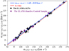 |
Fig. 1. Stellar velocity dispersion results, which are calculated from the CaT and CO (2-0) absorption features. Some of sources are not still observed for our entire sample, therefore, the sources for which our sample includes both σCaT and σCO(2-0) estimates are compared. The red solid line represents 1:1 line, whereas the blue solid line shows the offset between the σCaT and σCO(2-0) estimates of our data. The LLAMA AGNs and inactive galaxies are presented as black and purple, respectively. |
4.2. Robustness of stellar velocity dispersion estimations
Recent studies report that stellar velocity dispersion estimates can be affected by AGN contamination (Greene & Ho 2006b; Harris et al. 2012; Woo et al. 2013; Batiste et al. 2017b). Firstly, we address the question of whether the AGN continuum affects the stellar velocity dispersion estimations. In optical bands, the AGN continuum behaves like a power-law function (Oke et al. 1984) and can be defined as fλ ∝ λ−(αv + 2), where αv is the arithmetic mean of the power-law index. We adopt αv = −2.45 (Vanden Berk et al. 2001) to model a synthetic AGN continuum. First, we selected an inactive control galaxy (NGC 1315) from the LLAMA sample; the stellar velocity dispersion of this galaxy is estimated as σ⋆ = 77 ± 5 km s−1 using pPXF. Then, the synthetic AGN continuum was combined with the NGC 1315 spectrum. As expected, the AGN continuum has no direct effect on the σ⋆ estimations for any reasonable AGN continuum level (< 70%), if the continuum is modeled using an adequate number of additive polynomials. In the top panel of Fig. 2, we present a synthetic AGN spectrum, which consists of the spectrum of the inactive galaxy NGC 1315 (shown as red line) and a fairly strong (∼70%) model AGN continuum (blue line). Our active galaxies typically show a much smaller AGN contribution than 70% at the CaT, which is why this serves as a good test for our fitting accuracy.
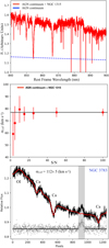 |
Fig. 2. Top: example of the spectrum from the control galaxy NGC 1315, which is combined with the model AGN continuum. The assumed AGN continuum are presented as the red and the blue, respectively. Middle: stellar velocity dispersion estimates relative to the S/N of the AGN continuum for NGC 1315 (red). The solid black line represents the stellar velocity dispersion estimate from the X-shooter spectrum, which has a S/N ∼ 44 per pixel. Bottom: example of pPXF fit for NGC 3783. Position of the O I emission line and the CaT absorption lines are demonstrated in the plot for visual aid. The gray masked feature represents the Fe II emission line at 8616 Å. |
On the other hand, the continuum level cannot be estimated accurately, if the spectrum is noisy. To test this, we applied a Monte Carlo approach to generate noise for every pixel of the synthetic AGN spectra. In this approach, a normal distribution of numbers are allowed to vary within a specified range, and the test was repeated 104 times to obtain the mean distribution of each noise level (S/N: 3, 5, 10, 15, 25, 50, 100). For each S/N level, we fit the data 102 times using pPXF. The stellar velocity dispersion estimates are obtained from the mean of the Gaussian distribution of resulting σ⋆ values for each S/N. In Fig. 2 (middle), we present the comparison between S/N and σ⋆ estimates. By considering this result, we can achieve reliable σ⋆ estimations using data with high S/N (> 15). We confirm that S/N is one of the most important factors, leading to an uncertainty of up to 20% for a S/N ≲ 5, which needs to be included into the total uncertainty of σ⋆. We note that our sample of AGNs are observed with S/N > 40; therefore, our calculations are not affected by this issue.
Moreover, AGN emission lines can also affect σ⋆ estimations. The broad O I (8446 Å) emission line, which is detected for some of the AGNs in our sample, is a good example of this (see the bottom Fig. 2). Correspondingly, we modeled an extremely broad O I 8446 Å line using a Gaussian model (σO I ∼ 2500 km s−1), which we added to the synthetic AGN spectrum. By fitting spectra around the CaT regime with different noise levels, we find evidence that the broad O I 8446 Å emission line can cause inaccurate stellar velocity dispersion estimations of up to 15%. Since the existence of a broad emission line affects the continuum level determination, such AGNs with broad O I 8446 Å have been treated specially by masking the part of the spectrum that is affected by the emission line. In a few cases, this can cut off the first CaT line (8498 Å), but we report that this does not affect the determination of the stellar velocity dispersion.
For disk galaxies, the galaxy rotation makes an important contribution to the measured stellar velocity dispersion from a larger aperture. The rotational dynamics of spiral galaxies are characterized by the total luminosity, line of sight, and maximum rotation velocities of the galaxy and the inclination angle of the disk (Tully & Fisher 1977). Since the LLAMA AGN sample is dominated by spiral galaxies, the galaxy rotation is another effect that may affect the stellar velocity dispersion estimates. By using the velocity-shifted SINFONI data cubes from Shimizu et al. (in prep.), we obtained an average inclination-corrected rotational velocity for the LLAMA sample. The contribution from the rotational effects are further discussed in Sect. 4.7.
4.3. Robustness of broad-line-based MBH estimates
We investigated the broad-line emission of our sample of Type 1 AGNs using two different apertures: 0 6 × 0
6 × 0 6 (the central region) and 1
 8 × 4″ (the FOV of X-shooter data). For each AGN, we fit Hα and Hβ emission lines with the same number of the Gaussian curves for each aperture. In Fig. 3, we present FWHM comparisons between the central region and the FOV. The broad-line FWHM estimates are found to differ up to 5% as a consequence of aperture choice. This difference can be related to the observational seeing or the narrow-line contamination. Since we cannot detect the entire BLR gas, this is a systematic error of FWHM estimates and should be added to total uncertainty budget of FWHM estimates.
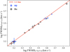 |
Fig. 3. Resulting FWHM comparisons for the small (0 |


The emission line width of a broad line can be obtained either from the FWHM or line dispersion (σLine). A typical AGN emission line profile can be described by a single Gaussian profile, and FWHM/σLine has a fixed ratio of 2 in the Gaussian profile. However, some of AGN emission line widths can only be modeled with multiple Gaussians. In this case, the FWHM needs to be estimated from the combined Gaussian models, and the ratio of FWHM to σLine can vary (Peterson et al. 2004; Peterson 2011). Peterson & Bontà (2018) argue that estimations based on σLine MBH are more accurate than those based on FWHM for Hβ, if an AGN emission has an irregular line profile. For the multiple-peaked emission line profiles, the irregular kurtosis can be either positive or negative, and it can affect the accuracy of emission line estimations. These authors also note that estimations based on σLine are less sensitive to the contribution from extended line wings. The σLine can be estimated from the second moment of the emission line profile P (λ) as follows:
![Mathematical equation: $$ \begin{aligned} \sigma _{\rm Line} = \left[\int \frac{(\lambda - \lambda _{0})^{2} P(\lambda ) \mathrm{d}\lambda }{\int P (\lambda ) \mathrm{d}\lambda }\right]^{1/2}, \end{aligned} $$](/articles/aa/full_html/2020/02/aa36321-19/aa36321-19-eq39.gif) (13)
(13)
where λ0 is the center of emission line profile. In Fig. 4, we compare the σLine obtained from the Eq. (13) and σModel obtained from its ratio with the FWHM (FWHM/σModel ≈ 2.355) for the Gaussian profile. We find a slight difference (an offset of 76.7 ± 56.2 km s−1) between the two estimates for our Hβ-based investigations. We note that this difference affects our MBH estimates by ∼0.1 dex. This result is consistent with Peterson & Bontà (2018), therefore, we also suggest using σLine in investigations based on HβMBH.
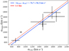 |
Fig. 4. Comparison between σLine, which is obtained from the Eq. (13) and σGauss, which is obtained from the line width of Gaussian model. |
4.4. Black hole masses and the systematical uncertainties
The MBH values for our sample of Type 1 AGNs are presented in Table 3. They are in the range 6.34 ≤ log MBH ≤ 7.75 M⊙ for Hα. We note that the average black hole mass of inactive galaxies in the relation by Kormendy & Ho (2013) is substantially higher, possibly indicating that our sample of AGNs did not yet go through a major merger phase (Wandel et al. 1999).
Black hole mass uncertainties are determined from the bootstrapping analysis. In this approach, we used all uncertainties from the parameters, such as uncertainties from single-epoch calibration parameters, f factor, FWHM, and luminosity. First, we generated 108 random numbers from a normal distribution for each parameter. Then, these numbers were added to all parameters of MBH estimations. Finally, using the Gaussian distribution of obtained 108 MBH values, we measured black hole mass uncertainties within the 1σ confidence level.
However. single-epoch based MBH estimations have been reported to have a systematical uncertainty, which is reported as a lower limit of 0.40 dex by (e.g., Pancoast et al. 2014). The uncertainty of f factor introduces an uncertainty of 0.12 dex (Woo et al. 2015), which is obtained from the comparison of the MBH–σ⋆ relation between the RM AGNs and inactive galaxies. The second uncertainty is the intrinsic scatter of BLR radius-luminosity relation, which is reported as 0.13 dex for reliable estimates (Bentz et al. 2013). Third, the variability in luminosity and line width bring a 0.1 dex uncertainty (Park et al. 2012b). Last, we adopt an uncertainty of 0.15 dex, which is assumed to come from redshift-independent distance measurements. Correspondingly, the total uncertainty of MBH estimates can be 0.3−0.4 dex.
4.5. Accretion rates
Many properties of the AGN (e.g., the torus phenomenology, Wada 2012) are expected to depend on the Eddington ratio of the “central engine”. One of the main drivers of our study is to provide the Eddington ratio for the whole LLAMA sample.
We compute the accretion rates following Eqs. (8) and (10) and find them in the range 0.04 < Ṁ < 0.92 M⊙ yr−1 assuming an accretion efficiency of 10% (see Table 3). Using our estimated black hole masses, we further calculate the Eddington ratio λ following Eq. (9) for all of our AGNs. They are in the regime 0.004 ≤ λ ≤ 0.49. These results indicate that the most LLAMA AGNs are growing at a rate that is well below Eddington, although likely in the radiatively efficient regime via a geometrically thin, optically thick disk (Shakura & Sunyaev 1973).
4.6. LLAMA sample MBH–σ⋆ relation
In Fig. 5, we present the MBH–σ⋆ relation for the LLAMA AGN sample adopting the broad-line-based single-epoch black hole masses derived using the Hα emission line profiles. Using the high S/N data, we report 38 stellar velocity dispersion estimates (20 AGNs and 18 inactive galaxies) in total (Table 2), which are derived from the CaT and/or CO (2-0) absorption features. We provide MBH of 10 Type 1 AGNs in the LLAMA sample (see Table 3). In addition, we adopt a stellar kinematic MBH estimate of NGC 5128 (Cappellari et al. 2009) and two megamaser MBH estimates of NGC 4388 (Greene et al. 2016) and NGC 5728 (Braatz et al. 2015). Therefore, we constructed an MBH–σ⋆ relation for 13 AGNs in the LLAMA sample.
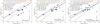 |
Fig. 5. Left: MBH − σ⋆ relation of our sample of galaxies, where MBH values are estimated using the Hα-based calibration. The MBH–σ⋆ relation of KH13, MM13, and W15 are presented as red, green, and blue solid lines, respectively. Sy 1.8, Sy 1.9, Sy 2, and LINER galaxies are presented in different colors for visual aid. The location of the two LLAMA Seyfert 2 (NGC 4388 and NGC 5728) galaxies are shown that have megamaser MBH estimates as blue triangles. In addition, we present the MBH estimates of NGC 5128 obtained from stellar kinematics as an orange box (Cappellari et al. 2009). Finally, the average uncertainties on the black hole mass estimates of the LLAMA AGNs (∼0.40 dex) are presented as a vertical black line in the legend to avoid confusion of data points. Middle: MBH–σ⋆ relation of our sample of galaxies, where MBH values are estimated using the extinction-corrected fluxes and the Hα calibration. Right: MBH–σ⋆ relation of our sample of galaxies, where the Hα MBH values are presented as the extinction-corrected and σ⋆ values are presented as rotation-corrected. The LLAMA MBH–σ⋆ relation is presented as a black dashed line. |
We then performed a linear regression in which we allowed both the intercept and the slope to vary. For this fit, we used FITEXY and the extinction-corrected MBH and the rotation-corrected σ⋆ estimates for our sample. We excluded NGC 7213 from this fit since it shows LINER-like properties; also the Hβ fit for this galaxy fails.
The resulting MBH–σ⋆ relation for the LLAMA AGNs is written as
 (14)
(14)
and the intrinsic scatter of this relation is ϵ = 0.32 ± 0.06. We note that our slope (3.38±0.65) is smaller than the slope reported by Woo et al. (2015) (3.97 ± 0.56) who included narrow-line Seyfert AGNs in order to extend to lower black hole masses; our slope is consistent with Woo et al. (2013) who found a slope of 3.46 ± 0.61. Within the uncertainties of our small sample, our slope is consistent with both of these AGN relations, but not consistent with the slope reported by Kormendy & Ho (2013) for more massive, inactive galaxies. This result still shows that the LLAMA sample of AGNs, which is a volume complete sample of the most luminous local AGNs, is representative for the larger AGN population sampled with RM in terms of its location and slope on the M-sigma relation.
For reference for future publication, and using the LLAMA MBH–σ⋆ relation (Eq. (14)), we also estimate MBH values for our Type 2 AGNs (Table 3).
4.7. LLAMA MBH–σ⋆ relation versus spheroidal MBH–σ⋆ relation
In the left panel of Fig. 5, we present the MBH values without extinction correction and σ⋆ parameter without rotation correction. We compare the LLAMA MBH–σ⋆ relation with the MBH–σ⋆ relation of KH13, MM13 and the AGN MBH–σ⋆ relation by W15. First, we found a high offset (0.75 dex) from the KH13 relation using these parameters.
In previous works, some authors concentrated on correcting the broad Balmer fluxes and/or the monochromatic accretion luminosities in various wavelengths (i.e., 1350, 3000, 5100 Å), which are used in single-epoch MBH estimations, using Galactic extinction maps (e.g., Vestergaard & Peterson 2006; Denney et al. 2009; Shen & Liu 2012; Bentz et al. 2016; Kozłowski 2017). In our study, we additionally corrected Hα and the continuum fluxes, which are used for deriving black hole masses, using the estimated BLR extinction of LLAMA sample by Schnorr-Müller et al. (2016). In the middle panel of Fig. 5, we present the MBH–σ⋆ relation obtained using extinction-corrected black hole masses. The extinction correction increased the estimated MBH by a factor of 0.02−0.93 dex for our sample, and reduced the average offset from the KH13 relation to 0.38 dex. This result indicates that the extinction in BLR can cause significantly under-estimation of MBH, unless it is taken into account.
In an upcoming LLAMA study, Shimizu et al. (in prep.) fit for the spatially resolved stellar kinematics within the SINFONI cubes. The stellar velocity fields are then modeled as an exponential disk. Using the model velocity field, we then shifted the spectra within the original SINFONI cubes such that the stellar velocity is removed. In this way, we can measure a rotation-corrected stellar velocity dispersion for the whole SINFONI FOV and compare this to the original value to produce a rotation correction that can be applied to our velocity dispersion based on X-shooter. Correspondingly, we obtain a rotation-correction factor for our AGNs (see Table 2). Therefore, we reduced the obtained stellar velocity dispersion using this rotation-correction factor. However, We are still missing SINFONI observations for the following galaxies: MCG-05-14-12, NGC 4235, NGC 5128, and the spatially resolved stellar kinematics for NGC 3783, MCG-06-30-15. For these galaxies, the obtained stellar velocity dispersion estimates are reduced 10% the average galaxy rotation contribution to σ⋆ for the LLAMA sample (Shimizu et al. in prep.). After the σ⋆ estimates are corrected for galaxy rotation, the LLAMA galaxies are found to agree with the MBH–σ⋆ relation of Kormendy & Ho (2013). The average intrinsic scatter of LLAMA sample obtained adopting the slope and intercept of Kormendy & Ho (2013) relation is found to be is 0.30 dex, which is consistent with the intrinsic scatter of the Kormendy & Ho (2013)MBH–σ⋆ relation (see Fig. 5). This result shows that the rotation can make a significant contribution to stellar velocity dispersion (up to 20%), which is consistent with previous investigations (e.g., Kang et al. 2013; Batiste et al. 2017a; Eun et al. 2017).
We additionally compared our results with the MBH–σ⋆ relation reported by MM13. By adopting a slope of 5.64 reported by MM13, we find an average offset of 0.46 dex for our sample relative to the relation of MM13. However, the majority of our sample (8 out of 10) are found to be above the relation reported by MM13. There are two possible explanations for the discrepancy between our results and MM13; in the MM13 sample, the disk galaxies are not corrected for their rotation component, and their sample includes brightest cluster galaxies, which are located in a different environment than the LLAMA sample.
Even though a few studies in the literature report that pseudo-bulges do not follow the MBH–σ⋆ relation (Greene et al. 2010; Kormendy et al. 2011; Kormendy & Ho 2013), the pseudo-bulge-dominated LLAMA sample follows the MBH–σ⋆ relation of elliptical and spheroidal bulge-dominated galaxies after applying the extinction correction to our MBH and the rotation correction to our σ⋆ estimates. Therefore, we argue that to reduce the offset from the elliptical-dominated MBH–σ⋆ relation, a correction to MBH for the dust extinction (derived via the Hα or continuum flux) and a correction of σ⋆ for a rotational component of the disk/bulge must be applied to spiral-dominated local Seyfert AGNs.
5. Conclusions
In a volume-limited complete sample of the most luminous, X-ray selected, local Sy 1 AGNs, comprising the LLAMA sample, we examine the spatially resolved stellar kinematics and the properties of the broad emission lines using medium spectral resolution (R ∼ 8000) X-shooter data. We additionally compare our results with SINFONI data, which extend our analysis to the H+K bands. Our main results are as follows:
-
We obtain the stellar velocity dispersions via the CaT at ∼8500 Å; these are in the range 73 ≤ σ⋆CaT ≤ 227 km s−1. We also estimate the stellar velocity dispersions from the NIR stellar CO (2-0) absorption feature for a subset of galaxies using SINFONI data and find them to be in the range 101 ≤ σ⋆CO(2-0) ≤ 231 km s−1. For the galaxies for which we have both observations, the two stellar velocity dispersion measurements are in good agreement. On average, the stellar velocity dispersion derived from the NIR CO feature is higher by ∼3.69 ± 0.93 km s−1 than the value derived from the CaT.
-
We apply Monte Carlo-like simulations to test the robustness of stellar velocity dispersion estimations for bright AGNs in which we test the effects of S/N and of the AGN continuum and emission lines. We conclude that stellar velocity dispersions can be obtained accurately for AGNs if the data have a S/N > 15.
-
We derive the SMBH masses of the LLAMA sample of Seyfert 1 AGNs from broad-line-based black hole mass estimates, which result in 6.34 ≤ log MBH ≤ 7.75 M⊙ using the Hα line width and flux as a tracer of black hole mass. We additionally estimate Hβ emission line black hole masses for our sample of AGNs. When the Hβ was not available, we use the Paβ emission line instead (see Table 3).
-
We find the Eddington ratio and accretion rates of the LLAMA sample to be within 0.004 ≤ λ ≤ 0.49 and 0.04 < Ṁ < 0.92 M⊙ yr−1, respectively. The median for Type 1 and Type 2 is ∼0.08 less than expected of Seyfert galaxies (10%), but perhaps consistent with the selection method (hard X-ray).
-
We find the best-fitting parameters for the LLAMA MBH–σ⋆ relation are α = 8.14 ± 0.20, β = 3.38 ± 0.65, ϵ = 0.32 ± 0.06. Within our uncertainties, the LLAMA AGN sample is consistent with the MBH–σ⋆ relations reported by Woo et al. (2013, 2015) in terms of slope. The average intrinsic scatter of LLAMA sample around the Kormendy & Ho (2013)MBH–σ⋆ relation is found to be 0.30 dex. This intrinsic scatter is consistent with the intrinsic scatter of the Kormendy & Ho (2013)MBH–σ⋆ relation. Correspondingly, we report that the pseudo-bulge-dominated LLAMA AGNs are now on the MBH–σ⋆ relation reported by Kormendy & Ho (2013) (see the right panel of Fig. 5).
-
We infer black hole masses for the other LLAMA Seyfert 2 AGNs as well as the inactive galaxies in the sample using the MBH–σ⋆ relation of the LLAMA AGNs with single-epoch RM or maser black hole masses.
-
We argue that to reduce the offset from the elliptical-dominated MBH–σ⋆ relation, a correction to MBH for the dust extinction (derived via the Hα or continuum flux) and a correction of σ⋆ for a rotational component of the disk/bulge must be applied to spiral-dominated local Seyfert AGNs. Our main finding implies that the MBH–σ⋆ relation could be same for both elliptical and pseudo-bulge hosting galaxies. Correspondingly, we encourage further investigations with larger samples.
Acknowledgments
We would like to thank the anonymous referee for the comments and suggestions. TC would like to thank Hojin Cho, Stefano Marchesi, Federica Ricci, Julián Mejía-Restrepo, Murillo Marinello Assis de Oliveira, Swayamtrupta Panda, Nathen Nguyen, Kimberly Emig, Kirsty Butler, Fraser Evans, Dirk van Dam and Walter Jaffe for very useful discussions. T. C. is partly supported by a DFG grant within the SPP 1573 “Physics of the interstellar medium”. R. A. R. thanks partial support from Conselho Nacional de Desenvolvimento Científico e Tecnológico and Fundação de Amparo à pesquisa do Estado do RS. S. V. acknowledges support from a Raymond and Beverley Sackler Distinguished Visitor Fellowship and thanks the host institute, the Institute of Astronomy, where this work was concluded. S. V. also acknowledges support by the Science and Technology Facilities Council (STFC) and by the Kavli Institute for Cosmology, Cambridge. VNB gratefully acknowledge assistance from a National Science Foundation (NSF) Research at Undergraduate Institutions (RUI) grant AST-1909297. Note that findings and conclusions do not necessarily represent views of the NSF.
References
- Abuter, R., Schreiber, J., & Eisenhauer, F. 2006, New A Rev., 50, 398 [Google Scholar]
- Akritas, M. G., & Bershady, M. A. 1996, ApJ, 470, 706 [NASA ADS] [CrossRef] [Google Scholar]
- Astropy Collaboration (Robitaille, T. P., et al.) 2013, A&A, 558, A33 [NASA ADS] [CrossRef] [EDP Sciences] [Google Scholar]
- Astropy Collaboration (Price-Whelan, A. M., et al.) 2018, AJ, 156, 123 [Google Scholar]
- Baggett, W. E., Baggett, S. M., & Anderson, K. S. J. 1998, AJ, 116, 1626 [NASA ADS] [CrossRef] [Google Scholar]
- Rothberg, B., & Fischer, J. 2010, ApJ, 712, 318 [NASA ADS] [CrossRef] [Google Scholar]
- Baumgartner, W. H., Tueller, J., Markwardt, C., & Skinner, G. 2010, BAAS, 42, 675 [Google Scholar]
- Barth, A. J., Greene, J. E., & Ho, L. C. 2005, ApJ, 619, 151 [NASA ADS] [CrossRef] [Google Scholar]
- Beifiori, A., Courteau, S., Corsini, E. M., & Zhu, Y. 2012, MNRAS, 419, 2497 [NASA ADS] [CrossRef] [Google Scholar]
- Batiste, M., Bentz, M. C., Raimundo, S. I., Vestergaard, M., & Onken, C. A. 2017a, ApJ, 838, 10 [Google Scholar]
- Batiste, M., Bentz, M. C., Manne-Nicholas, E. R., Onken, C. A., & Bershady, M. A. 2017b, ApJ, 835, 271 [NASA ADS] [CrossRef] [Google Scholar]
- Bentz, M. C., Denney, K. D., Cackett, E. M., et al. 2006, ApJ, 651, 775 [NASA ADS] [CrossRef] [Google Scholar]
- Bentz, M. C., Walsh, J. L., Barth, A. J., et al. 2009a, ApJ, 705, 199 [NASA ADS] [CrossRef] [Google Scholar]
- Bentz, M. C., Peterson, B. M., Netzer, H., Pogge, R. W., & Vestergaard, M. 2009b, ApJ, 697, 160 [Google Scholar]
- Bentz, M. C., Denney, K. D., Grier, C. J., et al. 2013, ApJ, 767, 149 [NASA ADS] [CrossRef] [Google Scholar]
- Bentz, M. C., Cackett, E. M., Crenshaw, D. M., et al. 2016, ApJ, 830, 136 [NASA ADS] [CrossRef] [Google Scholar]
- Bian, W.-H., & Zhao, Y.-H. 2003, PASJ, 55, 599 [NASA ADS] [CrossRef] [Google Scholar]
- Blandford, R., & McKee, C. F. 1982, ApJ, 255, 419 [NASA ADS] [CrossRef] [EDP Sciences] [Google Scholar]
- Braatz, J., Condon, J., Constantin, A., et al. 2015, IAU Gen. Assem., 22, 2255730 [NASA ADS] [Google Scholar]
- Burtscher, L., Davies, R. I., Graciá-Carpio, J., et al. 2016, A&A, 586, A28 [NASA ADS] [CrossRef] [EDP Sciences] [Google Scholar]
- Capetti, A. 2007, Balmaverde, B., 469, 88 [Google Scholar]
- Cappellari, M. 2017, MNRAS, 466, 798 [NASA ADS] [CrossRef] [Google Scholar]
- Cappellari, M., & Emsellem, E. 2004, PASP, 116, 138 [NASA ADS] [CrossRef] [Google Scholar]
- Cappellari, M., Neumayer, N., Reunanen, J., et al. 2009, MNRAS, 394, 660 [NASA ADS] [CrossRef] [Google Scholar]
- Chen, Y.-P., Trager, S. C., Peletier, R. F., et al. 2014, A&A, 565, A117 [NASA ADS] [CrossRef] [EDP Sciences] [Google Scholar]
- Collin, S., & Huré, J.-M. 2001, A&A, 372, 50 [NASA ADS] [CrossRef] [EDP Sciences] [Google Scholar]
- Collin, S., Kawaguchi, T., Peterson, B. M., & Vestergaard, M. 2006, A&A, 456, 75 [NASA ADS] [CrossRef] [EDP Sciences] [Google Scholar]
- Combes, F., Garcá-Burillo, S., Audibert, A., et al. 2019, A&A, 623, A79 [NASA ADS] [CrossRef] [EDP Sciences] [Google Scholar]
- Davidson, K. 1972, ApJ, 171, 213 [NASA ADS] [CrossRef] [Google Scholar]
- Davies, R. I., Burtscher, L., Rosario, D., et al. 2015, ApJ, 806, 127 [NASA ADS] [CrossRef] [Google Scholar]
- Davies, R. I., Hicks, E. K. S., Erwin, P., et al. 2017, MNRAS, 466, 4917 [NASA ADS] [CrossRef] [Google Scholar]
- de Lapparent, V., Baillard, A., & Bertin, E. 2011, A&A, 532, A75 [NASA ADS] [CrossRef] [EDP Sciences] [Google Scholar]
- Denney, K. D., Bentz, M. C., Peterson, B. M., et al. 2006, ApJ, 653, 152 [NASA ADS] [CrossRef] [Google Scholar]
- Denney, K. D., Peterson, B. M., Dietrich, M., Vestergaard, M., & Bentz, M. C. 2009, ApJ, 692, 246 [NASA ADS] [CrossRef] [Google Scholar]
- Denney, K. D., Peterson, B. M., Pogge, R. W., et al. 2010, ApJ, 721, 715 [NASA ADS] [CrossRef] [Google Scholar]
- Eun, D.-I., Woo, J.-H., & Bae, H.-J. 2017, ApJ, 842, 5 [NASA ADS] [CrossRef] [Google Scholar]
- Falcón-Barroso, J., Lyubenova, M., van de Ven, G., et al. 2017, A&A, 597, A48 [NASA ADS] [CrossRef] [EDP Sciences] [Google Scholar]
- Ferrarese, L., & Ford, H. 2005, Space Sci. Rev., 116, 523 [NASA ADS] [CrossRef] [Google Scholar]
- Ferrarese, L., & Merritt, D. 2000, ApJ, 539, 9 [Google Scholar]
- Fisher, D. B., & Drory, N. 2010, ApJ, 716, 2 [Google Scholar]
- Fisher, D. B., & Drory, N. 2016, in Galactic Bulges, eds. E. Laurikainen, R. Peletier, & D. Gadotti (Berlin: Springer), 41 [NASA ADS] [CrossRef] [Google Scholar]
- Freudling, W., Romaniello, M., Bramich, D. M., et al. 2013, A&A, 559, A96 [NASA ADS] [CrossRef] [EDP Sciences] [Google Scholar]
- Gadotti, D. A. 2008, MNRAS, 384, 420 [NASA ADS] [CrossRef] [Google Scholar]
- Gebhardt, K., Bender, R., Bower, G., & Stern, D. 2000, ApJ, 539, 13 [Google Scholar]
- Graham, A. W., Onken, C. A., Athanassoula, E., & Combes, F. 2011, MNRAS, 412, 2211 [NASA ADS] [CrossRef] [Google Scholar]
- GRAVITY Collaboration (Sturm, E., et al.) 2018, Nature, 563, 657 [Google Scholar]
- Greene, J. E., & Ho, L. C. 2005, ApJ, 630, 122 [NASA ADS] [CrossRef] [Google Scholar]
- Greene, J. E., & Ho, L. C. 2006a, ApJ, 641, 21 [Google Scholar]
- Greene, J. E., & Ho, L. C. 2006b, ApJ, 641, 117 [NASA ADS] [CrossRef] [Google Scholar]
- Greene, J. E., Peng, C. Y., & Kim, M. 2010, ApJ, 721, 26 [NASA ADS] [CrossRef] [Google Scholar]
- Greene, J. E., Seth, A., Kim, M., et al. 2016, ApJ, 826, 32 [Google Scholar]
- Grier, C. J., Peterson, B. M., Pogge, R. W., et al. 2012, ApJ, 755, 60 [NASA ADS] [CrossRef] [Google Scholar]
- Grier, C. J., Peterson, B. M., Horne, K., et al. 2013a, ApJ, 764, 47 [NASA ADS] [CrossRef] [Google Scholar]
- Grier, C. J., Martini, P., Watson, L. C., et al. 2013b, ApJ, 773, 90 [CrossRef] [Google Scholar]
- Grier, C. J., Pancoast, A., Barth, A. J., et al. 2017, ApJ, 849, 146 [NASA ADS] [CrossRef] [Google Scholar]
- González-Martín, O., Masegosa, J., Marquez, I., et al. 2015, A&A, 578, A74 [NASA ADS] [CrossRef] [EDP Sciences] [Google Scholar]
- Gao, H., Ho, L. C., Barth, A. J., & Li, Z.-Y. 2019, ApJS, 244, 34 [NASA ADS] [CrossRef] [Google Scholar]
- Gu, Q., Melnick, J., Fernandes, R. C., et al. 2006, MNRAS, 366, 480 [NASA ADS] [CrossRef] [Google Scholar]
- Gültekin, K., Richstone, D. O., Gebhardt, K., et al. 2009, ApJ, 698, 198 [NASA ADS] [CrossRef] [Google Scholar]
- Harris, C. E., Bennert, V. N., Auger, M. W., et al. 2012, ApJS, 201, 29 [NASA ADS] [CrossRef] [Google Scholar]
- Hu, C., Wang, J.-M., Ho, L. C., et al. 2016, ApJ, 832, 197 [NASA ADS] [CrossRef] [Google Scholar]
- Kang, W.-R., Woo, J.-H., Schulze, A., et al. 2013, ApJ, 767, 26 [NASA ADS] [CrossRef] [Google Scholar]
- Kaspi, S., Smith, P. S., Netzer, H., et al. 2000, ApJ, 533, 631 [NASA ADS] [CrossRef] [Google Scholar]
- King, A. 2003, ApJ, 596, 27 [Google Scholar]
- Knapen, J. H., de Jong, R. S., Stedman, S., & Bramich, D. M. 2003, MNRAS, 344, 527 [NASA ADS] [CrossRef] [Google Scholar]
- Koss, M., Trakhtenbrot, B., Ricci, C., et al. 2017, ApJ, 850, 74 [NASA ADS] [CrossRef] [Google Scholar]
- Kormendy, J., & Ho, C. L. 2013, ARA&A, 51, 511 [Google Scholar]
- Kormendy, J., Bender, R., & Cornell, M. N. 2011, Nature, 469, 374 [NASA ADS] [CrossRef] [Google Scholar]
- Kormendy, J., Drory, N., Bender, R., & Cornell, M. E. 2015, ApJ, 723, 1 [Google Scholar]
- Kozłowski, S. 2017, ApJS, 228, 9 [NASA ADS] [CrossRef] [Google Scholar]
- La Franca, F., Onori, F., Ricci, F., et al. 2015, MNRAS, 449, 1526 [NASA ADS] [CrossRef] [Google Scholar]
- Landt, H., Ward, M. J., Peterson, B. M., et al. 2013, MNRAS, 432, 113 [NASA ADS] [CrossRef] [Google Scholar]
- Laurikainen, E., Salo, H., Buta, R., Knapen, J. H., & Comerón, S. 2010, MNRAS, 405, 1089 [NASA ADS] [Google Scholar]
- Lynden-Bell, D. 1969, Nature, 223, 690 [NASA ADS] [CrossRef] [Google Scholar]
- Lin, M.-Y., Davies, R. I., Hicks, E. K. S., et al. 2018, MNRAS, 473, 4582 [NASA ADS] [CrossRef] [Google Scholar]
- Marinucci, A., Bianchi, S., Nicastro, F., Matt, G., & Goulding, A. D. 2012, ApJ, 748, 130 [NASA ADS] [CrossRef] [Google Scholar]
- McConnell, N. J., & Ma, C.-P. 2013, ApJ, 764, 184 [NASA ADS] [CrossRef] [Google Scholar]
- Maiolino, R., & Rieke, G. H. 2013, ApJ, 454, 95 [Google Scholar]
- Merritt, D., & Ferrarese, L. 2001, ApJ, 547, 140 [NASA ADS] [CrossRef] [Google Scholar]
- Mejía-Restrepo, J. E., Trakhtenbrot, B., Lira, P., Netzer, H., & Capellupo, D. M. 2016, MNRAS, 460, 187 [NASA ADS] [CrossRef] [Google Scholar]
- Mejía-Restrepo, J. E., Lira, P., Netzer, H., Trakhtenbrot, B., & Capellupo, D. M. 2018, Nat. Astron., 2, 63 [NASA ADS] [CrossRef] [Google Scholar]
- Modigliani, A., Goldoni, P., Royer, F., et al. 2010, Proc. SPIE, 7737, 28 [Google Scholar]
- Nelson, C. H., Green, R. F., Bower, G., Gebhardt, K., & Weistrop, D. 2004, ApJ, 615, 652 [NASA ADS] [CrossRef] [Google Scholar]
- Netzer, H. 1990, in Active Galactic Nuclei, eds. R. D. Blandford, H. Netzer, L. Woltjer, T. J. L. Courvoisier, & M. Mayor (Berlin: Springer-Verlag), 57 [Google Scholar]
- Netzer, H., Elitzur, M., & Ferland, G. J. 1990, ApJ, 299, 752 [NASA ADS] [CrossRef] [Google Scholar]
- Neumayer, N. 2010, PASA, 27, 449 [NASA ADS] [CrossRef] [Google Scholar]
- Oke, J. B., Shields, G. A., & Korycansky, D. G. 1984, ApJ, 277, 64 [NASA ADS] [CrossRef] [Google Scholar]
- Onken, C. A., & Peterson, B. M. 2002, ApJ, 572, 746 [NASA ADS] [CrossRef] [Google Scholar]
- Onken, C. A., Ferrarese, L., Merritt, D., et al. 2004, ApJ, 615, 645 [NASA ADS] [CrossRef] [Google Scholar]
- Osterbrock, D. E., & Ferland, G. J. 2006, Astrophysics of Gaseous Nebulae and Active Galactic Nuclei (Sausalito, CA: University Science Books) [Google Scholar]
- Osterbrock, D. E., & Pogge, R. W. 1985, ApJ, 297, 166 [NASA ADS] [CrossRef] [Google Scholar]
- Padovani, P., Alexander, D. M., Assef, R. J., et al. 2017, A&ARv, 25, 2 [Google Scholar]
- Pancoast, A., Brewer, B. J., Treu, T., et al. 2014, MNRAS, 445, 3073 [NASA ADS] [CrossRef] [Google Scholar]
- Park, D., Kelly, B. C., Woo, J.-H., & Treu, T. 2012a, ApJS, 203, 6 [NASA ADS] [CrossRef] [Google Scholar]
- Park, D., Woo, J.-H., Treu, T., et al. 2012b, ApJ, 747, 30 [NASA ADS] [CrossRef] [Google Scholar]
- Peterson, B. M. 1993, PASP, 105, 247 [NASA ADS] [CrossRef] [Google Scholar]
- Peterson, B. M. 2007, ASP Conf. Ser., 373, 3 [NASA ADS] [Google Scholar]
- Peterson, B. M. 2011, Proceedings of the Workshop “Narrow-Line Seyfert Galaxies and their Place in the Universe”, PoS(NLS1)032 [Google Scholar]
- Peterson, B. M., & Bontà, E. D. 2018, Proceedings of the Workshop “Narrow-Line Seyfert Galaxies and their Place in the Universe”, PoS(NLS1)032 [Google Scholar]
- Peterson, B. M., Ferrarese, L., Gilbert, K. M., et al. 2004, ApJ, 613, 682 [NASA ADS] [CrossRef] [Google Scholar]
- Press, W. H., Teukolsky, S. A., Vetterling, W. T., & Slannery, B. P. 1992, Numerical Recipes in C. The Art of Scientific Computing, Second Edition (Cambridge, New York, New Rochelle, Melbourne and Sydney: Cambridge University Press) [Google Scholar]
- Rosario, D. J., Burtscher, L., Davies, R. I., et al. 2018, MNRAS, 473, 5658 [NASA ADS] [CrossRef] [Google Scholar]
- Rosario, D. J., Togi, A., Burtscher, L., et al. 2019, ApJ, 875, 8 [Google Scholar]
- Ricci, C., Trakhtenbrot, B., Koss, M. J., et al. 2017a, ApJS, 233, 17 [NASA ADS] [CrossRef] [Google Scholar]
- Ricci, F., La Franca, F., Onori, F., & Bianchi, S. 2017b, A&A, 598, A51 [Google Scholar]
- Riffel, R. A., Ho, L. C., Mason, R., et al. 2015, MNRAS, 446, 2823 [NASA ADS] [CrossRef] [Google Scholar]
- Rybicki, G. B., & Lightman, A. P. 1986, Radiative Processes in Astrophysics (New York: Wiley-VCH), 400 [Google Scholar]
- Saglia, R. P., Opitsch, M., Erwin, P., et al. 2016, ApJ, 818, 47 [NASA ADS] [CrossRef] [Google Scholar]
- Salo, H., Laurikainen, E., Laine, J., et al. 2015, ApJS, 219, 4 [NASA ADS] [CrossRef] [Google Scholar]
- Shimizu, T. T., Davies, R. I., Koss, M., et al. 2018, ApJ, 856, 154 [NASA ADS] [CrossRef] [Google Scholar]
- Shimizu, T. T., Davies, R. I., Lutz, D., et al. 2019, MNRAS, 490, 5860 [NASA ADS] [CrossRef] [Google Scholar]
- Silge, J. D., & Gebhardt, K. 2003, AJ, 125, 2809 [NASA ADS] [CrossRef] [Google Scholar]
- Silk, J., & Rees, M. J. 1998, A&A, 331, 1 [Google Scholar]
- Schnorr-Müller, A., Davies, R. I., Korista, K. T., et al. 2016, MNRAS, 462, 3570 [NASA ADS] [CrossRef] [Google Scholar]
- Shakura, N. I., & Sunyaev, R. A. 1973, A&A., 24, 337 [NASA ADS] [Google Scholar]
- Shankar, F., Bernardi, M., & Sheth, R. K. 2016, MNRAS, 460, 3119 [NASA ADS] [CrossRef] [Google Scholar]
- Shankar, F., Bernardi, M., Richardson, K., et al. 2019, MNRAS, 485, 1278 [NASA ADS] [CrossRef] [Google Scholar]
- Shen, Y., & Liu, X. 2012, ApJ, 753, 125 [NASA ADS] [CrossRef] [Google Scholar]
- Shen, J., Vanden Berk, D. E., Schneider, D. P., & Hall, P. B. 2008, AJ, 135, 928 [NASA ADS] [CrossRef] [Google Scholar]
- Storchi-Bergmann, T., & Schnorr-Müller, A. 2019, Nat. Astron., 3, 48 [NASA ADS] [CrossRef] [Google Scholar]
- Storchi-Bergmann, T., Schimoia, J. S., Peterson, B. M., et al. 2017, ApJ, 835, 236 [NASA ADS] [CrossRef] [Google Scholar]
- Subramanian, S., Ramya, S., Das, M., et al. 2016, MNRAS, 455, 3148 [NASA ADS] [CrossRef] [Google Scholar]
- Skrutskie, M. F., Cutri, R. M., Stiening, R., et al. 2006, AJ, 131, 1163 [NASA ADS] [CrossRef] [Google Scholar]
- Terlevich, E., Diaz, A. I., & Terlevich, R. 1990, MNRAS, 242, 271 [NASA ADS] [CrossRef] [Google Scholar]
- Tremaine, S., Gebhardt, K., Bender, R., et al. 2002, ApJ, 574, 740 [NASA ADS] [CrossRef] [Google Scholar]
- Tully, R. B., & Fisher, J. R. 1977, A&A, 54, 661 [NASA ADS] [Google Scholar]
- Vanden Berk, D. E., Richards, G. T., Bauer, A., et al. 2001, AJ, 122, 549 [NASA ADS] [CrossRef] [Google Scholar]
- van den Bosch, R. C. E., Gebhardt, K., Gültekin, K., Yıldırım, A., & Walsh, J. L. 2015, ApJS, 218, 10 [NASA ADS] [CrossRef] [Google Scholar]
- van den Bosch, R. C. E. 2016, ApJ, 831, 134 [NASA ADS] [CrossRef] [Google Scholar]
- van der Marel, R. P., & Franx, M. 1993, ApJ, 407, 525 [NASA ADS] [CrossRef] [Google Scholar]
- Véron, M.-P., & Véron, P. 2010, A&A, 518, A10 [NASA ADS] [CrossRef] [EDP Sciences] [Google Scholar]
- Wada, K. 2012, ApJ, 758, 66 [NASA ADS] [CrossRef] [Google Scholar]
- Wandel, A., Peterson, B. M., & Malkan, M. A. 1999, ApJ, 526, 579 [NASA ADS] [CrossRef] [Google Scholar]
- Vestergaard, M., & Peterson, B. M. 2006, ApJ, 641, 689 [NASA ADS] [CrossRef] [Google Scholar]
- Wild, V., Groves, B., Heckman, T., et al. 2011, MNRAS, 410, 1593 [NASA ADS] [Google Scholar]
- Winge, C., Riffel, R. A., & Storchi-Bergmann, T. 2009, ApJS, 185, 186 [NASA ADS] [CrossRef] [Google Scholar]
- Winter, L., Veilleux, S., McKernan, B., & Kallman, T. 2012, ApJ, 745, 107 [NASA ADS] [CrossRef] [Google Scholar]
- Woo, J.-H., Treu, T., & Barth, A. J. 2010, ApJ, 716, 269 [NASA ADS] [CrossRef] [Google Scholar]
- Woo, J.-H., Schulze, A., Park, D., et al. 2013, ApJ, 772, 49 [NASA ADS] [CrossRef] [Google Scholar]
- Woo, J.-H., Yoon, Y., Park, S., Park, D., & Kim, S. C. 2015, ApJ, 801, 38 [NASA ADS] [CrossRef] [Google Scholar]
- Yoshino, A., & Yamauchi, C. 2015, MNRAS, 446, 3749 [NASA ADS] [CrossRef] [Google Scholar]
- Yu, Q., & Lu, Y. 2004, ApJ, 610, 93 [NASA ADS] [CrossRef] [Google Scholar]
Appendix A: Broad-Line fittings
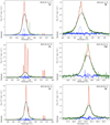 |
Fig. A.1. Broad-line region emission fittings of our sample. The black solid line represents the broad-line emission line width, whereas the red solid line represents the best fit. Residuals are shown in blue for visual aids. The unidentified blue-shifted broad emission lines of NGC 1365, NGC 2992 and MCG-05-14-12 are presented as blue dashed line. |
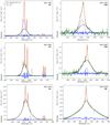 |
Fig. A.1. continued. |
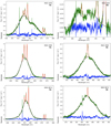 |
Fig. A.1. continued. |
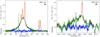 |
Fig. A.1. continued. |
Appendix B: The pPXF fittings
We present the pPXF stellar velocity dispersion fitting results from CaT absorption lines (from Fig. B.1), whereas CO (2-0) fitting results are presented from Fig. B.2.
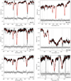 |
Fig. B.1. Fitting plots via pPXF for CaT. The red solid line represents the best fit, whereas the residuals are shown as gray. The vertical gray lines represent masked features. |
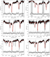 |
Fig. B.1. continued. |
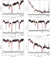 |
Fig. B.1. continued. |
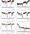 |
Fig. B.1. continued. |
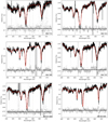 |
Fig. B.1. continued. |
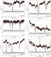 |
Fig. B.1. continued. |
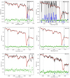 |
Fig. B.2. Fitting plots via pPXF for CO (2-0). The red solid line represents the best fit, whereas the residuals are shown as green. The vertical gray lines represent masked features. |
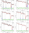 |
Fig. B.2. continued. |
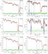 |
Fig. B.2. continued. |
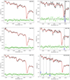 |
Fig. B.2. continued. |
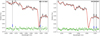 |
Fig. B.2. continued. |
All Tables
Galaxy properties: X-shooter, and SINFONI observation lists of our sample of galaxies.
Stellar velocity dispersion comparison between the estimates from CaT and CO (2-0) absorption lines.
All Figures
|
Fig. 1. Stellar velocity dispersion results, which are calculated from the CaT and CO (2-0) absorption features. Some of sources are not still observed for our entire sample, therefore, the sources for which our sample includes both σCaT and σCO(2-0) estimates are compared. The red solid line represents 1:1 line, whereas the blue solid line shows the offset between the σCaT and σCO(2-0) estimates of our data. The LLAMA AGNs and inactive galaxies are presented as black and purple, respectively. |
| In the text | |
|
Fig. 2. Top: example of the spectrum from the control galaxy NGC 1315, which is combined with the model AGN continuum. The assumed AGN continuum are presented as the red and the blue, respectively. Middle: stellar velocity dispersion estimates relative to the S/N of the AGN continuum for NGC 1315 (red). The solid black line represents the stellar velocity dispersion estimate from the X-shooter spectrum, which has a S/N ∼ 44 per pixel. Bottom: example of pPXF fit for NGC 3783. Position of the O I emission line and the CaT absorption lines are demonstrated in the plot for visual aid. The gray masked feature represents the Fe II emission line at 8616 Å. |
| In the text | |
|
Fig. 3. Resulting FWHM comparisons for the small (0 |
| In the text | |
|
Fig. 4. Comparison between σLine, which is obtained from the Eq. (13) and σGauss, which is obtained from the line width of Gaussian model. |
| In the text | |
|
Fig. 5. Left: MBH − σ⋆ relation of our sample of galaxies, where MBH values are estimated using the Hα-based calibration. The MBH–σ⋆ relation of KH13, MM13, and W15 are presented as red, green, and blue solid lines, respectively. Sy 1.8, Sy 1.9, Sy 2, and LINER galaxies are presented in different colors for visual aid. The location of the two LLAMA Seyfert 2 (NGC 4388 and NGC 5728) galaxies are shown that have megamaser MBH estimates as blue triangles. In addition, we present the MBH estimates of NGC 5128 obtained from stellar kinematics as an orange box (Cappellari et al. 2009). Finally, the average uncertainties on the black hole mass estimates of the LLAMA AGNs (∼0.40 dex) are presented as a vertical black line in the legend to avoid confusion of data points. Middle: MBH–σ⋆ relation of our sample of galaxies, where MBH values are estimated using the extinction-corrected fluxes and the Hα calibration. Right: MBH–σ⋆ relation of our sample of galaxies, where the Hα MBH values are presented as the extinction-corrected and σ⋆ values are presented as rotation-corrected. The LLAMA MBH–σ⋆ relation is presented as a black dashed line. |
| In the text | |
|
Fig. A.1. Broad-line region emission fittings of our sample. The black solid line represents the broad-line emission line width, whereas the red solid line represents the best fit. Residuals are shown in blue for visual aids. The unidentified blue-shifted broad emission lines of NGC 1365, NGC 2992 and MCG-05-14-12 are presented as blue dashed line. |
| In the text | |
|
Fig. A.1. continued. |
| In the text | |
|
Fig. A.1. continued. |
| In the text | |
|
Fig. A.1. continued. |
| In the text | |
|
Fig. B.1. Fitting plots via pPXF for CaT. The red solid line represents the best fit, whereas the residuals are shown as gray. The vertical gray lines represent masked features. |
| In the text | |
|
Fig. B.1. continued. |
| In the text | |
|
Fig. B.1. continued. |
| In the text | |
|
Fig. B.1. continued. |
| In the text | |
|
Fig. B.1. continued. |
| In the text | |
|
Fig. B.1. continued. |
| In the text | |
|
Fig. B.2. Fitting plots via pPXF for CO (2-0). The red solid line represents the best fit, whereas the residuals are shown as green. The vertical gray lines represent masked features. |
| In the text | |
|
Fig. B.2. continued. |
| In the text | |
|
Fig. B.2. continued. |
| In the text | |
|
Fig. B.2. continued. |
| In the text | |
|
Fig. B.2. continued. |
| In the text | |
Current usage metrics show cumulative count of Article Views (full-text article views including HTML views, PDF and ePub downloads, according to the available data) and Abstracts Views on Vision4Press platform.
Data correspond to usage on the plateform after 2015. The current usage metrics is available 48-96 hours after online publication and is updated daily on week days.
Initial download of the metrics may take a while.