| Issue |
A&A
Volume 634, February 2020
|
|
|---|---|---|
| Article Number | A10 | |
| Number of page(s) | 13 | |
| Section | Extragalactic astronomy | |
| DOI | https://doi.org/10.1051/0004-6361/201936136 | |
| Published online | 28 January 2020 | |
Kinematic and metallicity properties of the Aquarius dwarf galaxy from FORS2 MXU spectroscopy⋆⋆⋆
1
Instituto de Astrofísica de Andalucía – CSIC, Glorieta de la Astronomía s/n, 18008 Granada, Spain
e-mail: lhermosa@iaa.es
2
Instituto de Astrofísica de Canarias, C/ Vía Láctea s/n, 38205 La Laguna, Tenerife, Spain
3
Departamento de Astrofísica, Universidad de La Laguna, 38205 La Laguna, Tenerife, Spain
4
Institute of Astronomy, University of Cambridge, Madingley Road, Cambridge CB3 0HA, UK
5
European Southern Observatory, Karl-Schwarzschild Strasse 2, 85748 Garching, Germany
6
Max Planck Institute for Astronomy, Königstuhl 17, 69117 Heidelberg, Germany
7
School of Natural Sciences, University of Tasmania, Private Bag 37 Hobart, Tasmania 7001, Australia
8
Institute of Physics, Laboratory of Astrophysics, École Polytechnique Fédérale de Lausanne (EPFL), 1290 Sauverny, Switzerland
9
GEPI, CNRS UMR 8111, Observatoire de Paris, PSL Research University, 92125 Meudon, Cedex, France
10
National Research Council, Herzberg Institute of Astrophysics, 5071 West Saanich Road, Victoria, BC V9E 2E7, Canada
11
Leibniz-Institut für Astrophysik Potsdam (AIP), An der Sternwarte 16, 14482 Potsdam, Germany
12
Kapteyn Astronomical Institute, University of Groningen, 9700 AV Groningen, The Netherlands
Received:
19
June
2019
Accepted:
28
November
2019
Context. Dwarf galaxies found in isolation in the Local Group (LG) are unlikely to have interacted with the large LG spirals, and therefore environmental effects such as tidal and ram-pressure stripping should not be the main drivers of their evolution.
Aims. We provide insight into the internal mechanisms shaping LG dwarf galaxies by increasing our knowledge of the internal properties of isolated systems. Here we focus on the evolved stellar component of the Aquarius dwarf galaxy, whose kinematic and metallicity properties have only recently started to be explored.
Methods. Spectroscopic data in the region of the near-infrared Ca II triplet lines has been obtained with FORS2 at the Very Large Telescope for 53 red giant branch (RGB) stars. These data are used to derive line-of-sight (l.o.s.) velocities and [Fe/H] of the individual RGB stars.
Results. We derive a systemic velocity of −142.2+1.8−1.8 km s−1, in agreement with previous determinations from both the HI gas and stars. The internal kinematics of Aquarius appears to be best modelled by a combination of random motions (l.o.s. velocity dispersion of 10.3+1.6−1.3 km s−1) and linear rotation (with a gradient −5.0+1.6−1.9 km s−1 arcmin−1) along a PA = 139+17−27 deg, broadly consistent with the optical projected major axis. This rotation signal is significantly misaligned or even counter-rotating to that derived from the HI gas. We also find the tentative presence of a mild negative metallicity gradient and indications that the metal-rich stars have a colder velocity dispersion than the metal-poor ones.
Conclusions. This work represents a significant improvement with respect to previous measurements of the RGB stars of Aquarius as it doubles the number of member stars already studied in the literature. We speculate that the misaligned rotation between the HI gas and evolved stellar component might have been the result of recent accretion of HI gas, or re-accretion after gas-loss due to internal stellar feedback.
Key words: techniques: spectroscopic / galaxies: dwarf / Local Group / galaxies: kinematics and dynamics / galaxies: abundances / galaxies: stellar content
Table A.2 and the averaged spectra are available at the CDS via anonymous ftp to cdsarc.u-strasbg.fr (130.79.128.5) or via http://cdsarc.u-strasbg.fr/viz-bin/cat/J/A+A/634/A10
© ESO 2020
1. Introduction
Dwarf galaxies are objects of great interest for galaxy formation and evolution studies because they are the smallest and most numerous galaxies in the Universe. The Local Group (LG) hosts a large number of these systems that can be studied in great detail; it is possible to gather information on the properties of their stellar components over most of the lifetimes of the galaxies by studying individual low-mass stars, such as red giant branch (RGB) stars.
The internal kinematic and metallicity properties of the classical (pre-SDSS) dwarf galaxies orbiting around the Milky Way (MW) have been well-studied due to the favorable combination of close distance, luminosity, and angular size that makes a perfect match for existing wide-area multi-object spectrographs. However, dwarf galaxies have relatively low masses and this arguably makes their evolution susceptible both to internal and external effects. The study of the LG dwarf galaxies found in isolation1 is therefore valuable as they offer a cleaner view than satellite galaxies of the internal mechanisms that have shaped the evolution of systems at the low end of the galaxy mass function. However, due to their larger distance from us, it is challenging to obtain large spectroscopic samples of individual RGB stars in these objects, and thus the internal kinematics and metallicity properties of their evolved stellar component have only started to be explored quite recently (see, e.g., Fraternali et al. 2009; Leaman et al. 2013; Kirby et al. 2014; Kacharov et al. 2017; Taibi et al. 2018).
Pinning down the characteristics of isolated LG dwarf galaxies can also inform models that try to explain what is known as the LG morphology-density relation: isolated LG dwarf galaxies mostly contain HI gas (late types), in stark contrast with satellite galaxies of M31 or the MW, which are mostly devoid of neutral gas (early types).
Historically, LG late-type dwarfs have been divided into dwarf irregulars (dIrrs) and transition types (dTs)2. The dTs contain a neutral gas component but no ongoing star formation, so that their properties are intermediate to those of dIrrs and early types such as dwarf spheroidals (dSphs). Because of this, it has been suggested that they are an evolutionary link between these two types (see, e.g., Tolstoy et al. 2009). On the other hand, dTs have also been considered as an extension of dIrrs with low star formation rate (Weisz et al. 2011; Koleva et al. 2013). It should be noted that the morphological classification is generally based on the dwarfs’ present-day properties, while it has been shown that dwarfs of the same type may have had different evolutionary pasts, as derived from their full star formation history (Gallart et al. 2015). This underlines the importance of referring to dwarf galaxies on the basis of their physical properties.
This work is part of a series of articles in which we make use of spectroscopic data of individual RGB stars to improve the observational picture of the properties of the evolved stellar component of isolated LG dwarf galaxies (Kacharov et al. 2017; Taibi et al. 2018, and in prep.). Here we focus on Aquarius (DDO 210; see Table 1 for a summary of its main properties). It is located near the edge of the LG, approximately 1 Mpc from the MW and 1.1 Mpc from M31 (for studies of distance based on RGB stars see van den Bergh et al. 1979; Lee et al. 1999; McConnachie et al. 2005), and only two galaxies are found within a distance of 500 kpc from it (SagDIG and VV124; Cole et al. 2014, and references therein). Its free-fall time to the barycenter of the LG is approximately equal to one Hubble time (McConnachie et al. 2006; McConnachie 2012), which means that it has likely not interacted with M31 or the MW during its lifetime. Moreover, the estimator of the tidal interactions of this galaxy with its closer neighbors is consistent with a system in isolation following the criteria from Karachentsev et al. (2004, 2013).
Parameters adopted for the Aquarius (DDO 210) dwarf galaxy.
The classification of this galaxy has varied: it has been referred to both as a dT (e.g., Mateo 1998; McConnachie et al. 2006) and as a dIrr (Cole et al. 2014, although they recognized its transition properties). It shows a higher fraction of gas mass to stellar mass with respect to the other systems classified as dTs, like Pegasus or Phoenix (see, e.g., McConnachie 2012). It has a clear UV surface brightness profile (Lee et al. 2009) that makes it more similar to systems classified as a dIrr. On the other hand, even though it has experienced a very prolonged star formation history, its star formation rate was higher between 6 and 8 Gyrs ago; it has declined over the last 2 Gyrs, and is currently almost null (Cole et al. 2014).
Stars in this galaxy were resolved for the first time by Marconi et al. (1990) reaching a magnitude of 23.5 in the V band. The stellar component presents a well-defined position angle and an ellipticity varying with radius, becoming more circular in the outer parts (McConnachie et al. 2006). The young stars (main sequence and blue loop stars), which are the least numerous, present a different surface density profile with respect to the older population (RGB and red clump stars). This indicates that the spatial distribution of star forming regions has varied over time (McConnachie et al. 2006). As for spectroscopy of the evolved stellar component, there are only two studies that have derived line-of-sight (l.o.s.) velocities and metallicities of individual stars (Kirby et al. 2014, 2017a).
The neutral gas properties are well-determined, showing that the morphologies of HI gas and stars differ (e.g., Young et al. 2003; Begum & Chengalur 2004; McConnachie et al. 2006). When overlaying the HI contours on optical images of Aquarius, it is clearly seen that they are not coincident (Young et al. 2003). This is mainly caused by the position of the young stars in the galaxy, shifted a few arcminutes to the east with respect to the center, and coincident with a small cavity in the HI profile as indicated by McConnachie et al. (2006). Although fewer, the young stars are brighter than the older ones, disproportionately impacting the surface brightness profile. This difference in the stellar distribution is probably causing the variation of ellipticity with radius. Both Young et al. (2003) and Begum & Chengalur (2004) reported a small velocity gradient in the HI gas and, more recently, this is confirmed by Iorio et al. (2017), who measure the velocity gradient along a PA = 77 deg.
Here we present results of our study of the chemical and kinematic properties of the stellar component of the Aquarius dwarf, based on VLT/FORS2 MXU spectroscopic observations in the region of the near-infrared Ca II triplet lines (nIR CaT) for a sample of 53 individual RGB stars. The article is structured as follows. In Sect. 2 we present the data acquisition and observational details. In Sect. 3 we describe the reduction process and the determination of velocities and metallicities for the whole sample. In Sect. 4 we apply selection criteria to identify likely member stars, and we perform the analysis of the kinematic properties of Aquarius. In Sect. 5 we analyze the metallicity distribution ([Fe/H]) and explore the possible presence of two different chemo-dynamical stellar populations. In Sect. 6 we discuss the main results and compare them with the characteristics of the neutral gas. The summary and our conclusions are in Sect. 7.
2. Observations
The data were obtained in service mode between June and September 2013 as part of the ESO Program 091.B-0331 (PI: G. Battaglia) using the FORS2 instrument at UT 1 of the Very Large Telescope (VLT). The targets were selected to have magnitudes and colors consistent with being RGB stars at the distance of the Aquarius dwarf galaxy. To that end, we used Subaru/SuprimeCam imaging data in the Johnson-Cousins V and I bands by McConnachie et al. (2006) from objects classified as point sources with high confidence. Slits to which we could not assign likely Aquarius RGB stars were allocated to random objects3. To ensure precise slit allocations, we used short pre-imaging exposures obtained with FORS2 within the same program.
Figure 1 shows the spectroscopic targets’ spatial distribution (left) and location on the Subaru/SuprimeCam color-magnitude diagram (right). We obtained 55 spectra for 53 individual objects distributed over two FORS2 MXU masks, each observed with ten exposures, for a total of 25 h. On average the airmass was around 1.1, and the seeing about 0.9″ for the Aquarius 0 mask and 1.1″ for Aquarius 1. We refer the reader to the observing log in Appendix A.1 for more details.
 |
Fig. 1. Spatial distribution (left) of the targets projected onto the tangential plane and color-magnitude diagram of the stars along the line of sight to Aquarius (right). Shown are the stars observed with VLT/FORS2 MXU and classified as Aquarius members (red circles), the sample of stars members from Kirby et al. (2017a) (blue squares), the stars in common between these two studies (yellow diamonds), and the VLT/FORS2 MXU RGB stars that have been classified as probable non-members of the galaxy (black crosses). In the left panel, the ellipse has a semi-major axis equal to 3 times the half-light radius of the galaxy, with a position angle of 99° and ellipticity of 0.5 (see Table 1). The black dot represents the galactic center. In the right panel, gray points represent the objects classified with high confidence as stars in the Subaru/SuprimeCam photometric data (34′×27′). Magnitudes have been corrected for extinction assuming a uniform Galactic screen and adopting E(B-V) from Table 1 along with reddening law AV = 3.1 × E(B − V). |
We adopted the same instrumental setup and observing strategy as in Kacharov et al. (2017) and Taibi et al. (2018; hereafter T18), where the chemo-dynamical properties of the stellar component of the Phoenix transition-type galaxy and the Cetus dwarf spheroidal galaxy have been studied. Mask slits were designed to be 1″ wide by 8″ long (for two slits, 6″ lengths were used to avoid overlap with adjacent slits). We used the 1028z+29 holographic grism in conjunction with the OG590+32 order separation filter to cover a wavelength range between 7700 − 9500 Å. This encompassed the region of the nIR CaT lines. The spectral dispersion was 0.84 Å pix−1 and the resolving power R = λcen/Δλ = 2560 at λcen = 8600 Å. Calibration data (biases, arc lamp, dome flat-field frames) and slit acquisition images were acquired as part of the FORS2 standard calibration plan.
3. Data reduction process and measurements
We adopted the same procedures described in Kacharov et al. (2017) and T18 for the data reduction, and for the determination of l.o.s. velocities and metallicities.
The optimally extracted, background-subtracted 1D spectra for each aperture were corrected for zero-point shifts due to the different date of observation, and possible small slit-centering shifts. Furthermore, the wavelength calibration was refined by exploiting the presence of numerous OH telluric emission lines.
The refinement to the wavelength calibration was obtained with the IRAF4fxcor task, through cross-correlation between a reference sky spectrum and the OH emission lines visible in the scientific exposures over the wavelength range 8200 − 9000 Å. The corrections ranged from ±1.2 − 16.9 km s−1 with errors ±0.7 − 2.9 km s−1. The slit-centering correction was calculated by comparing the position of the centroid of each slit with respect to the centroid of the stellar flux. The flux is measured in the through-slit images. If the target is not well centered on the slit, this causes a velocity offset (systematic wavelength shift) for targets that are smaller than or comparable in size to the slit width (Irwin & Tolstoy 2002). The computed correction ranged from ±0.15 − 8.5 km s−1 with errors ±0.4 − 4.2 km s−1. The short slit length of the two 6″ slits prevented a proper calculation of the slit-centering shift. Since the value of the slit-centering correction was found to change smoothly as a function of location on the chip, for these two stars we adopted the slit-centering correction of the adjacent targets. The barycentric correction was obtained using the IRAF rvcorrect task. All the shifts were applied to the individual spectra using the IRAF task dopcor.
3.1. Heliocentric velocity and metallicity measurements
The heliocentric velocities (vhel) and equivalent widths (EWs) for the CaT lines were measured on the stacked spectra, obtained from a weighted sum of the individual exposures. Table A.2 lists the S/N per pixel for each star, measured in the CaT region from the stacked spectra; the median S/N per pixel is 26. Figure 2 shows an example of two stacked spectra.
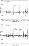 |
Fig. 2. Example spectra of the stars aqu0c1star2 (upper panel) and aqu1c2star3 (lower panel). The CaT lines and S/N for each spectra are indicated. |
To calculate the heliocentric l.o.s. velocity of the stars, we used again the IRAF task fxcor and cross-correlated the stacked spectra with an interpolated Kurucz stellar atmosphere model over the wavelength range 8400−8750 Å. The model was convolved to have the same dispersion as our data, and its parameters were chosen to represent a low-metallicity RGB star: log(g) = 1.0, Teff = 4000 K, [Fe/H] = −1.5 dex.
The CaT EWs were obtained from the continuum normalized stacked spectra by fitting a Voigt profile to the individual CaT lines, integrating their flux over a window of 15 Å and adopting the corresponding error spectra as the flux uncertainty at each pixel in the fitting process. To obtain estimates of the stars’ metallicity ([Fe/H]) we adopted the Starkenburg et al. (2010) relation as a function of the (V − VHB), linearly combining the EW of the two strongest CaT lines. The errors were calculated by propagation of the EW uncertainties. As a value for VHB we use 25.45 ± 0.20, estimated with photometric data from Cole et al. (2014); we verified that adopting the Starkenburg et al. (2010) calibration expressed as a function of the stars absolute visual magnitude leads to the same results. We note that CaT lines have been widely used to estimate the [Fe/H] of RGB stars in a variety of stellar systems, from MW globular and open clusters (see, e.g., Rutledge et al. 1997; Carrera 2012) to LG dwarf galaxies (see, e.g., Tolstoy et al. 2001; Battaglia et al. 2008), and tested and calibrated over a broad range of metallicities and stellar ages (see, e.g., Battaglia et al. 2008; Starkenburg et al. 2010; Carrera et al. 2013). Specifically, the validity of the Starkenburg et al. (2010) relation has been tested over the range −4 ≤ [Fe/H] ≤ −0.5.
Two stars in our sample were observed with both masks. The velocity and [Fe/H] for the two measurements were consistent within the errors in both cases. Therefore, we combined their velocities and [Fe/H] using a weighted mean for the final analysis, leading to a total number of 53 targets.
Table A.2 reports the slit information, RA-Dec coordinates, V- and I-band magnitudes, velocity, [Fe/H], S/N, and the membership status according to the criteria applied in Sect. 4 for each of the targets. The median error in the velocity and [Fe/H] measurements is 4.8 km s−1 and 0.13 dex respectively.
The spectra of four of our targets, labeled “C” in Table A.2, contain strong CN bands (see also Kirby et al. 2017a). For these we closely inspected the results from fxcor, which delivered a well-defined cross-correlation peak. Based on this, and given that (i) the velocities of these stars are close to the systemic velocity of the galaxy, (ii) their magnitudes are compatible with belonging to the RGB, and (iii) their metallicities do not stand out from the rest, we decided to include them in the final sample because they do not significantly bias our results.
3.2. Comparison with Kirby et al. (2017a)
Kirby et al. (2017a; hereafter K17) use Keck/DEIMOS spectroscopic data to measure heliocentric l.o.s. velocities (metallicities) for 25 (23) stars classified as Aquarius members. A search of matches within 2″ returns five overlapping stars with our sample. Table 2 lists the heliocentric velocities and [Fe/H] values for these stars in common: the star displaying the largest error in l.o.s. heliocentric velocity according to the determination of Kirby was measured twice in our sample (once with each mask), yielding measurements compatible within 1σ (see previous section) and was combined in the analysis (aqu0c1star11). The velocity derived for this star is compatible within 1σ in both studies. However, the measurements for the other four stars suggest the presence of a possible zero-point offset (∼10 km s−1) between the two studies. For perfectly derived velocity errors, we would expect the distribution of normalized velocity differences,  , to yield a mean of (0 ± 0.44) and a standard deviation of (1 ± 0.34) for a sample of five stars. In this case, the mean and standard deviation are 1.75 and 1.8, respectively, supporting the possibility that most of the velocity differences are not due to random errors. We note, however, that due to the small number of overlapping stars it is difficult to ascertain whether the only source of these differences is a systematic offset.
VLT/FORS2 and Keck/DEIMOS l.o.s. velocities and [Fe/H] for the stars in common between this work and Kirby et al. (2017a).
Offsets between radial velocity determinations of the same stars from different studies are not unusual. They happen not only when different spectrographs are used (see, e.g., Gregory et al. 2019 for a comparison of FORS2 multi-slit versus the FLAMES/GIRAFFE fiber observations of the Tucana dSph), but sometimes even when the same instrument and configuration mode are adopted (e.g., the comparison of Keck/DEIMOS R ∼ 6500 observations of the Triangulum II system; Kirby et al. 2017b). However, we have validated our data reduction and analysis procedure in multiple studies that included subsamples of repeated exposures for the same stars, which yielded consistent results. Since our methodology has not changed, we are confident that internally our velocity determinations are reliable.
For the metallicities, the FORS2 and DEIMOS measurements agree with each other within 1–2σ for four out of five stars. Given the different methods used (CaT EWs in one case and spectral synthesis excluding the CaT in the other), this is very encouraging. Star aqu0c1star11, which is the one that deviates the most in velocity, shows a large deviation in metallicity as well. The S/N of the DEIMOS spectra of this star is much lower than the typical S/N of the spectra for the rest of the sample (6 Å−1 versus a mean of ∼18 Å−1, with a corresponding dispersion of 5.7 Å pix−1), while its metallicity error is instead similar to that of the rest of the sample (0.16 dex). It is possible that the error quoted by K17 is underestimated for this star. In support of this statement, we note that there is another star in the K17 sample with a spectrum of S/N = 6 Å−1 and that has instead an error in [Fe/H] of 0.45 dex.
4. Kinematic analysis
4.1. Membership
In order to determine the kinematic and metallicity properties of the galaxy, we had to apply selection criteria to discard foreground contaminant stars along the line of sight to Aquarius.
We excluded the stars in two steps. First, we eliminated one star whose magnitude and color is not compatible with RGB stars at the distance of Aquarius. Then we performed a selection on the basis of the heliocentric velocity of the stars. We adopted  MAD(vhel) as a simple approach to exclude the targets5. The estimation of these parameters was an iterative process, fitting the data until convergence, and including the possible presence of rotation (see Sect. 4.2) at the same time. The data set was reduced from 52 to 46 targets. We double-checked this kinematic selection by applying a Bayesian analysis (see also Sect. 4.2) that solved iteratively the systemic velocity of the system vsys, the velocity dispersion σv, and the best-fitting model for the internal kinematics (dispersion-only or dispersion + rotation). We used this information to calculate the expected bulk velocity at the position of each given star (vbulk) and retained those targets that fulfilled the condition ∣vhel − vbulk ∣ ≤ 3 MAD(vhel − vbulk). This process excluded one more star from the sample, giving us a final number of 45 members. A histogram of the velocities for all targets and members is shown in Fig. 3.
 |
Fig. 3. Histogram of the heliocentric velocities of all the targets (black) and the 45 targets that were considered as members of the galaxy (blue). |
4.2. Internal kinematic properties
Wheeler et al. (2017) carried out a systematic analysis of the rotational support of LG dwarf galaxies, based on l.o.s. velocities from literature studies. One of the main aims of the authors was to understand whether the rotational support of the stellar component of LG late-type dwarf galaxies is significantly different from that of dSph satellites of the MW and M31, as would be predicted by the “tidal stirring model” put forward to explain the morphology-density relation of the LG (Mayer et al. 2001, 2006; Kazantzidis et al. 2011). For a full discussion of the importance of determining the internal kinematic properties of different classes of dwarf galaxies, we refer the reader to Wheeler et al. (2017) and Ivkovich & McCall (2019), among others. Here we explore these properties for our VLT/FORS2 sample of Aquarius stars.
Figure 4 offers a first look into this aspect by displaying the heliocentric l.o.s. velocities of Aquarius member stars as a function of the distance from the projected optical minor axis of the galaxy (see Table 1): a velocity gradient is clearly visible, with a weighted linear fit yielding a slope of −3.1 ± 1.0 km s−1 arcmin−1. The systemic velocity and velocity dispersion obtained are vsys = −139.9 ± 1.0 km s−1 and σv = 11.0 km s−1, respectively. A weighted linear fit to the vhel along the minor axis instead is consistent with no velocity gradient. Therefore, there are indications of a mild amount of rotation in this system. We note that Aquarius is an isolated galaxy with a small angular extent on the sky, so that it is highly unlikely that the detected velocity gradient is due to effects such as tidal disturbances or projection effects of the 3D motion of the galaxy across the line of sight.
 |
Fig. 4. Velocity distribution of the probable Aquarius members with respect to their distance to the minor axis. Shown are the best weighted linear fit to the stars’ velocities (solid blue line) and the systemic velocity derived from the fit (dashed line). |
We performed a Bayesian analysis in order to search for the presence of velocity gradients in Aquarius without fixing a preferred axis a priori (for more details on the methodology, see T18). The corresponding results are presented in Table 3. We compare three different models: a dispersion-only model, and a model including both random motions and rotation, expressed either as linear rotation or constant (flat) rotation velocity as a function of radius. The free parameters are the systemic velocity and velocity dispersion in the three models (vhel and σv, respectively); the position angle (θ) of the kinematic major axis for the two models with rotation; and the slope of the velocity gradient for the linear model (k) and the value of the rotational velocity for the flat model (vc). The results of the three models can be compared in terms of the Bayes factor (i.e., the ratio of the Bayesian evidence of a given model against the other: lnBlin, flat and lnBrot, disp). On the Jeffrey scale when the natural logarithm of the Bayes factor is (0–1),(1–2.5),(2.5–5), and (5+), the evidence can be interpreted as inconclusive, weak, moderate, and strong, respectively.
Parameters and evidence resulting from the application of the Bayesian analysis to the whole FORS2/MXU sample of members, as well as divided in metal-rich (MR) and metal-poor (MP) samples.
We find that the linear rotation model is weakly favored both with respect to the constant rotation model (lnBlin, flat = 1.7) and with respect to the dispersion-only model (lnBrot, disp = 1.6). The systemic velocity, dispersion and slope of the velocity gradient derived with this approach are, respectively,  km s−1,
  km s−1, and
  km s−1 arcmin−1 (
 km s−1 kpc−1), consistent within 1–2σ from the determinations obtained with a weighted linear fit to the velocities along the major axis. The best-fitting position angle of the kinematic major axis is
  degrees, shifted with respect to that of the projected major axis of the galaxy, although consistent with it at the 1.5σ level. In our definition, a negative velocity gradient with θ between 0° and 180° implies a receding velocity on the west side (and would be equivalent to a positive gradient with θ = θ + 180°).
Iorio et al. (2017) find a weak velocity gradient in the HI gas: they measure a rotational velocity of ∼5 km s−1 out to a radius of 1.5′ (using the distance they assumed to convert from kiloparsecs to arcminutes), similar to the rotational velocity we would obtain at approximately the same radius6. However, the kinematic major axis of the HI gas has a PA of 77.3 ± 15.2 degrees (receding velocities on the East side), which is misaligned with the kinematic PA of the stellar component here examined. In Sect. 4.4 we show that this misalignment is unlikely to be a consequence of the characteristics of the FORS2 data set in terms of number statistics, spatial coverage, and velocity uncertainties, and in Sect. 6 we discuss the possible origins of this feature, placing it in the context of the complexities of the structure and HI properties of Aquarius.
4.3. Comparison with other works
We have also applied our Bayesian analysis of the Aquarius internal kinematics to the smaller sample of 25 member stars by K17. This sample consists for the most part of re-observations of stars in Kirby et al. (2014; with 27 members, 24 of which in common with K17).
For the K17 data set, the comparison between the two rotational models does not clearly favor one over the other (lnBlin, flat = 0.13), and the comparison between the (slightly) favored linear rotation model against the dispersion-only model is lnBrot, disp = 0.28. Therefore, the presence of rotation cannot be proven conclusively from the K17 sample (see also Sect. 4.4). The lack of constraining power of the DEIMOS sample in terms of rotation signal is also consistent with the analysis by K17, who only placed a 95% confidence limit of a constant rotational velocity to be < 9 km s−1.
The presence of rotation in Aquarius has also been studied in Wheeler et al. (2017) using the Kirby et al. (2014) data set. The authors applied a similar Bayesian statistical analysis to ours, comparing a dispersion model, a constant rotation model, and a rotational model considering a radially varying pseudo-isothermal sphere. They found lnBlin, flat = −1.00 and lnBrot, disp = 0.62. The (weakly) favored model is the flat rotational model, although the Bayesian evidence on the presence of rotation is inconclusive.
We also applied our method to the sample of Kirby et al. (2014) and found similar results to those of Wheeler et al. (2017) (lnBlin, flat = −1.74 and lnBrot, disp = 0.97), despite the difference in one of the rotational models. We also recover closely the values of the best-fitting parameters in Wheeler et al. (2017). We note that the K17 data set gives the same results as the Kirby et al. (2014) sample, apart from a shift in systemic velocity.
4.4. Mock tests
We performed a series of tests on mock catalogues in order to understand what type of rotational properties can be detected, given the characteristics of the data sets available. To this end, we produced sets of mock l.o.s. velocities at the same position as the spectroscopically observed stars, which we analyzed in the same way as the actual data. These were extracted from Gaussian distributions centered on a vrot, mock and with standard deviation equal to the l.o.s. velocity error corresponding to that given star. The vrot, mock values at (x, y) position are obtained from the given rotational model under consideration (linear or flat), having vrot, mock/σmock = n = 1.5, 1.0, 0.75, 0.5, 0.25, 0 at twice the half-light radius (see Table 1); the velocity dispersion σmock was fixed to 10 km s−1 for all cases.
The simulated linear rotation models correspond to velocity gradients k = 6.8, 4.5, 3.4, 2.3, 1.1, and 0 km s−1 arcmin−1, while the constant rotation models had rotational velocities vc = 15, 10, 7.5, 5.0, 2.5, and 0 km s−1. All the cases were simulated for three different position angles that correspond to the P.A. of the projected semi-major axis of the stars (99°), then adding 45 and 90 degrees (semi-minor axis). Each case was simulated N = 1000 times. The experiments were run for the FORS2 MXU and the K17 samples; the Bayes factors for each n value, position angle, and model are shown in Fig. 5.
 |
Fig. 5. Bayes factor of the mock tests performed on the FORS2/MXU (left) and K17 (right) samples. Each panel represents the results for a different value of vrot, mock/σ, as given in the panel title. Squares and crosses refer to the linear and flat rotational model (LM, FM), respectively. The color of the markers (red, green, and blue) represents a different simulated position angle (99, 144, and 189 degrees, respectively). The purple circle indicates the Bayes factor derived for the real data sets (for the one referring to the K17 sample, see Sect. 4). Black solid lines discriminate between the strengths of the evidence for each case (yellow: strong; pink: moderate; green: weak; gray: inconclusive). |
Results from the tests indicate that rotation can be detected with at least a weak positive evidence when along the optical major axis of the galaxy for n ≥ 0.75 for the FORS2 data set and n ≥ 1 for the K17 sample. The two data sets have a similar sensitivity to the direction of rotation and model type in terms of ranking, with the FORS2 sample yielding greater evidence for a given model, and therefore a better capability to detect rotation at a given n. The data sets under consideration are not sensitive to the presence of low levels of rotation (n ≤ 0.5 for FORS2, n ≤ 0.75 for K17), since these return either inconclusive evidence or even weak evidence disfavoring the presence of rotation. In the dispersion-only case (n = 0) both samples favor this model versus the two models that include rotation, showing that there is no bias toward the rotational models.
In terms of strength of the lnBlin, flat evidence (see Fig. 5), the value derived for Aquarius stars observed with FORS2 appears compatible with a linear gradient, but not with a flat rotation model. This result could be a consequence of the fact that dwarf galaxies typically have slowly rising rotation curves, which do not always reach their flat part at the last measured point, as can be appreciated from the kinematics of the HI component (e.g., Oh et al. 2015; Iorio et al. 2017).
The underlying rotation could have rotational support n = 1.5 along the minor axis or intermediate PA, n = 1 along the intermediate axis or the major axis, or n = 0.75 along the major axis. For the K17 sample, the evidence in favor of one or the other rotational model is not so different from each other, and therefore a distinction does not appear possible. However, in terms of compatibility between the observed Bayes factor and levels of n and the direction of the gradient that might induce it, the outcome is similar to that of the FORS2 sample.
From our tests on the mock catalogues, we also extracted information on how well the kinematic major axis PA and the rotational velocity at a given radius are recovered for the various n (see Fig. 6). The initial values are always retrieved within the 99% confidence interval (C.I.), with a small bias toward underestimating the rotation when the kinematic major axis is along the optical minor axis. Also in terms of amplitude of the rotational velocity, the favored models would be those with n ≥ 0.75.
 |
Fig. 6. Rotation velocity at Rmax = 3′ vs. kinematic position angle recovered from the tests on mock catalogues reproducing the characteristics of the FORS2 data set and simulating a linear rotation model. Gray circles represent input values at n = 1.5, 1.0, 0.75, 0.5, 0.25, 0.; colored circles, squares, and triangles represent recovered values at different simulated kinematic PA; colors from blue to brown represent decreasing values of n, while the error bars are the 99% confidence interval (C.I.); in black the observed value from our data set with error bars at 68% C.I. |
It should be noted that the PA of the kinematic major axis for the observed RGB stars is beyond the 99% C.I. of that retrieved for the models with kinematics similar to that exhibited by the HI gas, indicating that the misalignment or counter-rotation of the stellar component and HI gas is not due to number statistics, spatial coverage, and measurement errors of our FORS2 data set.
5. Metallicity properties
The [Fe/H] values obtained for all FORS2 targets are listed in Table A.27. We derive the median of the metallicity distribution of all members of Aquarius to be [Fe/H] = − 1.59 ± 0.05 dex. This is compatible with the average value of ⟨[Fe/H]⟩ = −1.50 ± 0.06 dex by K17, and places Aquarius straight onto the luminosity-metallicity relation for Local Group dwarf galaxies (see Fig. 7). The spread measured as the MAD is 0.20 dex, while the intrinsic dispersion, taking into account the measurement errors and assuming a Gaussian form for the metallicity distribution function (MDF), is 0.25 dex. This value is at the low end, but is still compatible with the [Fe/H] dispersion of other Local Group dwarf galaxies (e.g., Leaman et al. 2013).
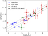 |
Fig. 7. Luminosity-stellar [Fe/H] relation for Local Group dwarf galaxies. Blue stars represent the MW-dSph satellites; red squares are M31-dSph satellites; green diamonds are dIrrs in the LG; the black circle is the position of Aquarius based on the [Fe/H] derived in this work; gray lines are the least-squares linear fit for the dIrrs and MW dSphs and the 0.16 scatter limits. All the values apart from Aquarius were taken from Kirby et al. (2013). |
Figure 8 shows the variation of [Fe/H] as a function of the elliptical (left) and circular (right) radius8. In this figure we also include the points from K17 since we have verified that their metallicity distribution function compares well with that from our FORS2 sample, as in general do the individual [Fe/H] measurements for the stars in common.
 |
Fig. 8. [Fe/H] as a function of the elliptical radius (left) and circular radius (right) for Aquarius member stars observed with FORS2 (red circles) and with DEIMOS (blue squares; Kirby et al. 2017a). The error bars show the uncertainties on the [Fe/H] measurements for the individual stars. The solid green line represents a running median boxcar with a kernel size of 7 points; the green band shows the 1σ error for the running median boxcar, taken as the standard deviation of 1000 Monte Carlo realizations of the running median itself, where the metallicities are extracted from Gaussians centered on the measured [Fe/H] of each star and dispersion given by the measurement uncertainty; the light green band is the same error band with the MDF intrinsic scatter added in quadrature. The black solid line represents the result of a Gaussian process regression analysis using a Gaussian kernel and taking into account an intrinsic scatter; the gray band indicates the corresponding 1σ confidence interval. |
It has been shown in the literature that a linear fit does not always fully capture the trend of spatial variations in the metallicity properties of Local Group dwarf galaxies; for example, in some systems a decline in the mean metallicity properties is followed by a flattening in the outer parts (see, e.g., Sextans, Battaglia et al. 2011; Cetus, T18). Therefore, we adopt more flexible ways to determine the general trend as a function of radius, such as a running median and a Gaussian-process (GP) regression. In order to take into account the effect of measurement errors (and of the intrinsic scatter), we obtain 1000 Monte Carlo realizations of the individual metallicities, extracting them from Gaussians centered at the observed values and with dispersion given by the metallicity errors (added in quadrature to the intrinsic scatter in the MDF). In the case of the GP regression, we use a Gaussian kernel together with a noise component to take into account the intrinsic scatter of the data. This method has the advantage of not depending on a fixed boxcar, like the running median, and the output has a probabilistic meaning. In both cases there is a very mild negative metallicity gradient. This is also seen when considering the run of the metallicity as a function of circular radius (not corrected for ellipticity). There are hints of a flattening of the slope at large radii; however, the current sample size does not allow us to draw firm conclusion. We have verified that considering only the FORS2 sample would lead to a very similar trend from the running median or the GP analysis.
Since the GP analysis returns a trend similar to a very simple linear relation, we performed a simple Bayesian linear regression, including an intrinsic scatter term, to estimate the significance of the metallicity gradient. The resulting cumulative posterior distribution of the slope of the metallicity gradient indicates that the possibility of no gradient is within 96% (∼1.75σ) and 94% (∼1.55σ) of the distribution, when considering the elliptical radius and the circular radius, respectively. So, while there are indications of a gradient, with this data set we cannot exclude a flat trend within 2σ in both cases.
From an observational point of view, should the presence of a metallicity gradient in an isolated dwarf galaxy such as Aquarius be strengthened in the future with larger data sets, it would lend further support to the hypothesis that negative metallicity gradients in Local Group dwarf galaxies are not to be ascribed to interactions with the large Local Group galaxies (see, e.g., the case of VV 124 and Phoenix; Kirby et al. 2012; Kacharov et al. 2017). Factors such as the dwarf galaxy’s star formation history, gravitational potential, and rotational versus dispersion support, as well as specific accretion events, are indeed expected to contribute to producing metallicity gradients (e.g., Marcolini et al. 2008; Schroyen et al. 2013; Benítez-Llambay et al. 2016; Revaz & Jablonka 2018). For satellite galaxies, it is possible that effects such as tidal and ram-pressure stripping of the gaseous component could modify the strength of such gradients, exacerbating them depending on the infall time onto the host halo versus the time when star formation ceased, or on the contrary blurring them in the case of strong tidal interactions (Sales et al. 2010). We defer to a future study the analysis of the possible correlations between rotational support and spatial variations of the metallicity properties of Local Group dwarf galaxies (Taibi et al. in prep.), along the lines of the work by Leaman et al. (2013).
The possible presence of a metallicity gradient has led us to look for subpopulations with different chemo-kinematic properties. We divided our data set into a metal-rich (MR) and a metal-poor (MP) sample based on the median [Fe/H] value of the entire set (22 and 23 stars, respectively). We then performed a Bayesian maximum likelihood analysis on both samples (see Sect. 4.2); the resulting parameters and evidence are reported in Table 3. We can see, independently from the fitted kinematic model, that the velocity dispersion values for the two samples are at ∼2σ from each other. We also note that the evidence of rotation has decreased, due to the low number of targets in each set. This tentative result of a spatially concentrated metal-rich population with a lower velocity dispersion compared to a spatially extended metal-poor one with a higher dispersion value, adds to what has already been found in several other dwarf galaxies of the LG (e.g., Tolstoy et al. 2004; Battaglia et al. 2006, 2008; Amorisco & Evans 2012; Breddels & Helmi 2014; Taibi et al. 2018). However, in our case we would benefit from a larger sample in order to place stronger constraints on the velocity dispersion of the MR and MP stars.
6. Discussion
In Fig. 9 we compare the structural and kinematic properties of the HI and stellar component of Aquarius.
 |
Fig. 9. Comparison between the HI (Iorio et al. 2017) and stellar (this work) velocity field. Left: Voronoi-binned stellar velocity field (S/N ∼ 3, see text for details); the gray contours show the HI surface density at 0.6, 1.2, 1.8, 2.4 M⊙ pc−2, with the lowest contour at 3σ above the noise (also shown in the middle and right panels). Middle: HI velocity field. Right: pixel-to-pixel difference between the stellar and HI velocity field; the small ellipse in the bottom right corner shows the beam of the HI observations. In the first two panels the circles represent the stars in our sample; the color indicates the vhel, and the size is proportional to vhel/δ vhel. In each panel the dashed ellipse is the same as Fig. 1, while the solid ellipse shows the PA and the inclination obtained through the analysis of the HI kinematics disk by Iorio et al. (2017). The cross indicates the galactic center (see Table 1). |
Iorio et al. (2017) found a weak velocity gradient in the HI gas whose amplitude is not dissimilar to what we measure for the stars at comparable radii, but with a kinematic major-axis of PA = 77.3 ± 15.2 degrees (in their definition this implies receding velocities on the east side). This velocity gradient is misaligned and counter-rotating with the kinematic PA of the stellar component, and with the PA of the surface density maps of the stellar and HI components (see ellipses in Fig. 9).
It is possible that the PA of the optical component is affected by the small fraction of bright young stars in Aquarius. On the other hand, Iorio et al. (2017) note that the HI map is quite peculiar with isodensity contours that are not elliptical. In fact, judging from Fig. 9, the density map of the HI component appears to have a PA of ∼130–140 degrees and there appears to be HI missing in the SE quadrant around that position angle (see also McConnachie et al. 2006). This might raise a question: If HI were present in this region, could the kinematic PA of the HI component be reconciled with the kinematic PA of the stars?
Nonetheless, it is clear that the HI gas and the RGB stars appear to counter-rotate: the former have the most negative velocities on the west side, while the latter display them on the east side. In Sect. 4.4 it was established that if the underlying kinematic properties of Aquarius stellar component were like the HI gas, there would be less than 1% probability of measuring the observed misalignment between the HI and stellar kinematic major axes.
In Fig. 9 we compare directly the stellar (left panel) and HI (middle panel) velocity fields. In order to make a pixel-by-pixel comparison of the velocity fields, we binned the Aquarius FORS2 members using the same pixel size of the HI map (1.5 arcsec). Then we applied a Voronoi binning technique increasing the Poisson S/N of each bin to 3 (≈9 star per Voronoi bin). The resultant velocity field for the stars is shown as colored areas in the left panel of Fig. 9. The presence of a velocity gradient is obvious, approximately along the stellar major axis in agreement with the results obtained in Sect. 4. The right panel of Fig. 9 shows the pixel-by-pixel difference between the stellar (left panel) and the HI velocity field (middle panel). The velocity difference is approximately 5 km s−1 along the HI PA and reaches ≈10 km s−1 close to the east and northwest edges of the HI disk.
This phenomenon of counter- or misaligned rotation of two different components of a galaxy has already been observed in the Local Group dwarf galaxy NGC 6822 (Demers et al. 2006) and systems outside the Local Group. The first event of counter-rotation was reported by Bettoni (1984) when studying the stellar and gas kinematics of six elliptical galaxies. It could be related to mergers with other galaxies that may have determined the internal evolution of the systems, to internal instabilities (Evans & Collett 1994) or to accretion of the gas, which should have produced star formation, so two different stellar populations can be differentiated (Pizzella et al. 2004).
Recently Starkenburg et al. (2019) tried to understand the origin of such counter-rotation using a large sample of low-mass galaxies (M⋆ ∼ 109 − 1010 M⊙) from the Illustris simulations. They found that only ∼1% of their sample showed signs of star–gas counter-rotation at the present time, when considering disks and spheroids together. The origin of counter-rotation was ascribed to a significant episode of gas-loss followed by the acquisition of new gas with misaligned angular momentum. They identified two main mechanisms for the gas removal: internally induced by a strong feedback burst or environmentally induced by a fly-by passage with a large host causing the gas stripping. On the other hand they found no significant relation between the counter-rotation and the presence of a major merger event. Taking into account the extreme isolation at which Aquarius is found, the hypothesis of the internally induced counter-rotation seems appealing. In Starkenburg et al. (2019), galaxies exhibiting counter-rotation were predominantly found among dispersion dominated systems. Given that in general Local Group dwarf galaxies in the Aquarius stellar mass range are not rotation supported, it is possible that in this regime the overall fraction of galaxies that could have experienced events resulting in counter-rotation of gas and stars could be larger than the 1% estimated in Starkenburg et al. (2019).
Iorio et al. (2017) find signs of a possible inflow or outflow of gas in Aquarius, as an extended region of HI emission along the minor axis not connected with the rotating HI disk. We postulate that in general the kinematics of the HI component in Aquarius might be dominated by recently accreted gas, while the RGB stars, which according to the Cole et al. (2014) SFH are likely to be dominated by ∼8 Gyr old stars, are tracing the kinematic properties as they were imprinted a much longer time ago along a different kinematic axis.
7. Summary and conclusions
We present an analysis of the kinematic and metallicity properties of the isolated Local Group dwarf galaxy Aquarius. The data set consisted of VLT/FORS2 MXU spectroscopic observations in the region of the near-IR CaT for 53 individual targets. The spectra have a median S/N of 26 pix−1 and led to the determination of l.o.s. velocities and [Fe/H] measurements with median uncertainties of ±4.8 and 0.13 dex, respectively. Of the 53 individual stars observed, 45 are probable RGB stars that are members of Aquarius, which doubles the number of RGB stars with l.o.s. velocities and [Fe/H] measurements available in the literature for this galaxy.
The systemic velocity derived for Aquarius is −142.2 ± 1.8 km s−1, in agreement with prior determinations from samples of individual stars (Kirby et al. 2017a) and also fully consistent with that of the HI component (Iorio et al. 2017). We find the internal kinematics of Aquarius to be best modelled by a combination of random motions (with l.o.s. velocity dispersion  km s−1) and linear rotation, with a velocity gradient of
  km s−1 arcmin−1 along an axis with PA
  degrees, broadly consistent (within 2σ) with the optical projected major axis of the galaxy.
On the other hand, the HI gas has a weak velocity gradient of comparable amplitude but along an axis with PA = 77.3 ± 15.2 degrees (Iorio et al. 2017). According to the definitions used in this work, this implies counter-rotation of the stellar and HI component.
We have run a set of mock tests to better understand the rotational properties that can be derived from the FORS2 data. The results of these tests indicate that such misalignment is not the result of the characteristics of our FORS2 data (number statistics, coverage, measurement errors). A direct comparison of the stars and HI velocity fields lends further support to the detection of such counter-rotation.
We speculate that the kinematics of the HI is dominated by recently accreted gas which is not tracing the kinematic properties of the RGB stars, the bulk of which are likely to have formed ≈8 Gyr ago (Cole et al. 2014) (although the observed sample is likely to be biased toward younger stars; Manning & Cole 2017). It is possible that this HI gas could simply be gas within Aquarius that was affected by particularly strong episodes of internal stellar feedback, rather than having been recently acquired from the intergalactic medium.
Finally, we characterized the metallicity properties of Aquarius. The median metallicity ([Fe/H] = − 1.59 ± 0.05 dex) indicates that it is a metal-poor galaxy, in agreement with the results from Kirby et al. (2017a). We analyzed the distribution of the metallicities as a function of radius, characterizing them through a running median and a Gaussian process regression; this shows the presence of a very mild negative metallicity gradient, with the more metal-rich stars found in the innerparts of the galaxy. Should the presence of such a gradient be confirmed with larger data sets, it would add to the number of isolated Local Group dwarf galaxies that display negative metallicity gradients and live in an environment where interactions with the large LG spirals cannot be invoked to explain these properties.
It is beyond the scope of this paper to review the taxonomy of dwarf galaxies, for which we refer the readers to other works in the literature (e.g., Tolstoy et al. 2009; Ivkovich & McCall 2019). There are no blue compact dwarfs in the LG, with the possible exception of IC 10.
IRAF is the Image Reduction and Analysis Facility distributed by the National Optical Astronomy Observatories (NOAO) for the reduction and analysis of astronomical data. http://iraf.noao.edu/
The authors quote the maximum circular velocity within the observed radial range as the data for Aquarius did not reach parts of the galaxy far enough out to include the flat part of the rotation curve. The value for the circular velocity, after the highly dominating asymmetric-drift correction, is V0 = 16.4 ± 9.5 km s−1.
The “elliptical radius” is the semi-major axis of the ellipse that passes through the (x, y) location of a given star and that has center, ellipticity, and PA as in Table 1; instead, the “circular radius” is simply (x2 + y2)1/2. Here x and y are the star’s projected celestial coordinates.
Acknowledgments
The authors thank the referee for a thorough report that has helped improving the manuscript. L.H.M. acknowledges financial support from the State Agency for Research of the Spanish MCIU through the “Center of Excellence Severo Ochoa” award for the Instituto de Astrofísica de Andalucía (SEV-2017-0709) and through the grants AYA2016-76682-C3 and BES-2017-082471. G.B. and S.T. acknowledge financial support through the grants (AEI/FEDER, UE) AYA2017-89076-P, AYA2014-56795-P, as well as by the Ministerio de Ciencia, Innovación y Universidades (MCIU), through the State Budget and by the Consejería de Economía, Industria, Comercio y Conocimiento of the Canary Islands Autonomous Community, through the Regional Budget. G.B. acknowledges financial support through the grant RYC-2012-11537. E.S. gratefully acknowledges funding by the Emmy Noether program from the Deutsche Forschungsgemeinschaft (DFG). This research has made use of NASA’s Astrophysics Data System, IRAF and Python, specifically with Astropy, (http://www.astropy.org), a community-developed core Python package for Astronomy (Astropy Collaboration 2013; Price-Whelan et al. 2018), Scipy, Matplotlib (Hunter 2007), Scikit-learn (Pedregosa et al. 2011) and PyMultinest (Buchner et al. 2014).
References
- Amorisco, N. C., & Evans, N. W. 2012, MNRAS, 419, 184 [NASA ADS] [CrossRef] [Google Scholar]
- Astropy Collaboration (Robitaille, T. P., et al.) 2013, A&A, 558, A33 [NASA ADS] [CrossRef] [EDP Sciences] [Google Scholar]
- Battaglia, G., Tolstoy, E., Helmi, A., et al. 2006, A&A, 459, 423 [NASA ADS] [CrossRef] [EDP Sciences] [Google Scholar]
- Battaglia, G., Irwin, M., Tolstoy, E., et al. 2008, MNRAS, 383, 183 [NASA ADS] [CrossRef] [MathSciNet] [Google Scholar]
- Battaglia, G., Tolstoy, E., Helmi, A., et al. 2011, MNRAS, 411, 1013 [NASA ADS] [CrossRef] [MathSciNet] [Google Scholar]
- Begum, A., & Chengalur, J. N. 2004, A&A, 413, 525 [NASA ADS] [CrossRef] [EDP Sciences] [Google Scholar]
- Benítez-Llambay, A., Navarro, J. F., Abadi, M. G., et al. 2016, MNRAS, 456, 1185 [NASA ADS] [CrossRef] [Google Scholar]
- Bettoni, D. 1984, The Messenger, 37, 17 [NASA ADS] [Google Scholar]
- Breddels, M. A., & Helmi, A. 2014, ApJ, 791, L3 [NASA ADS] [CrossRef] [Google Scholar]
- Buchner, J., Georgakakis, A., Nandra, K., et al. 2014, A&A, 564, A125 [NASA ADS] [CrossRef] [EDP Sciences] [Google Scholar]
- Carrera, R. 2012, A&A, 544, A109 [NASA ADS] [CrossRef] [EDP Sciences] [Google Scholar]
- Carrera, R., Pancino, E., Gallart, C., & del Pino, A. 2013, MNRAS, 434, 1681 [NASA ADS] [CrossRef] [Google Scholar]
- Cole, A. A., Weisz, D. R., Dolphin, A. E., et al. 2014, ApJ, 795, 54 [NASA ADS] [CrossRef] [Google Scholar]
- Demers, S., Battinelli, P., & Kunkel, W. E. 2006, ApJ, 636, L85 [NASA ADS] [CrossRef] [MathSciNet] [Google Scholar]
- Evans, N. W., & Collett, J. L. 1994, ApJ, 420, L67 [NASA ADS] [CrossRef] [Google Scholar]
- Fraternali, F., Tolstoy, E., Irwin, M. J., & Cole, A. A. 2009, A&A, 499, 121 [NASA ADS] [CrossRef] [EDP Sciences] [Google Scholar]
- Gallart, C., Monelli, M., Mayer, L., et al. 2015, ApJ, 811, L18 [NASA ADS] [CrossRef] [Google Scholar]
- Gregory, A. L., Collins, M. L. M., Read, J. I., et al. 2019, MNRAS, 485, 2010 [NASA ADS] [CrossRef] [Google Scholar]
- Hunter, J. D. 2007, Comput. Sci. Eng., 9, 90 [NASA ADS] [CrossRef] [Google Scholar]
- Iorio, G., Fraternali, F., Nipoti, C., et al. 2017, MNRAS, 466, 4159 [NASA ADS] [Google Scholar]
- Irwin, M., & Tolstoy, E. 2002, MNRAS, 336, 643 [NASA ADS] [CrossRef] [Google Scholar]
- Ivkovich, N., & McCall, M. L. 2019, MNRAS, 486, 1964 [NASA ADS] [CrossRef] [Google Scholar]
- Kacharov, N., Battaglia, G., Rejkuba, M., et al. 2017, MNRAS, 466, 2006 [NASA ADS] [CrossRef] [Google Scholar]
- Karachentsev, I. D., Karachentseva, V. E., Huchtmeier, W. K., & Makarov, D. I. 2004, AJ, 127, 2031 [Google Scholar]
- Karachentsev, I. D., Makarov, D. I., & Kaisina, E. I. 2013, AJ, 145, 101 [NASA ADS] [CrossRef] [Google Scholar]
- Kazantzidis, S., Łokas, E. L., Mayer, L., Knebe, A., & Klimentowski, J. 2011, ApJ, 740, L24 [NASA ADS] [CrossRef] [Google Scholar]
- Kirby, E. N., Bullock, J. S., Boylan-Kolchin, M., Kaplinghat, M., & Cohen, J. G. 2014, MNRAS, 439, 1015 [Google Scholar]
- Kirby, E. N., Cohen, J. G., & Bellazzini, M. 2012, ApJ, 751, 46 [NASA ADS] [CrossRef] [Google Scholar]
- Kirby, E. N., Cohen, J. G., Guhathakurta, P., et al. 2013, ApJ, 779, 102 [NASA ADS] [CrossRef] [Google Scholar]
- Kirby, E. N., Rizzi, L., Held, E. V., et al. 2017a, ApJ, 834, 9 [NASA ADS] [CrossRef] [Google Scholar]
- Kirby, E. N., Cohen, J. G., Simon, J. D., et al. 2017b, ApJ, 838, 83 [NASA ADS] [CrossRef] [Google Scholar]
- Koleva, M., Bouchard, A., Prugniel, P., De Rijcke, S., & Vauglin, I. 2013, MNRAS, 428, 2949 [NASA ADS] [CrossRef] [Google Scholar]
- Leaman, R., Venn, K. A., Brooks, A. M., et al. 2013, ApJ, 767, 131 [NASA ADS] [CrossRef] [Google Scholar]
- Lee, J. C., Gil de Paz, A., Tremonti, C., et al. 2009, ApJ, 706, 599 [NASA ADS] [CrossRef] [Google Scholar]
- Lee, M. G., Aparicio, A., Tikonov, N., Byun, Y.-I., & Kim, E. 1999, AJ, 118, 853 [NASA ADS] [CrossRef] [Google Scholar]
- Manning, E. M., & Cole, A. A. 2017, MNRAS, 471, 4194 [NASA ADS] [CrossRef] [Google Scholar]
- Marcolini, A., D’Ercole, A., Battaglia, G., & Gibson, B. K. 2008, MNRAS, 386, 2173 [NASA ADS] [CrossRef] [Google Scholar]
- Marconi, G., Focardi, P., Greggio, L., & Tosi, M. 1990, ApJ, 360, L39 [NASA ADS] [CrossRef] [Google Scholar]
- Mateo, M. L. 1998, ARA&A, 36, 435 [NASA ADS] [CrossRef] [Google Scholar]
- Mayer, L., Governato, F., Colpi, M., et al. 2001, ApJ, 547, L123 [NASA ADS] [CrossRef] [Google Scholar]
- Mayer, L., Mastropietro, C., Wadsley, J., Stadel, J., & Moore, B. 2006, MNRAS, 369, 1021 [NASA ADS] [CrossRef] [Google Scholar]
- McConnachie, A. W. 2012, AJ, 144, 4 [NASA ADS] [CrossRef] [Google Scholar]
- McConnachie, A. W., Irwin, M. J., Ferguson, A. M. N., et al. 2005, MNRAS, 356, 979 [NASA ADS] [CrossRef] [Google Scholar]
- McConnachie, A. W., Arimoto, N., Irwin, M., & Tolstoy, E. 2006, MNRAS, 373, 715 [NASA ADS] [CrossRef] [Google Scholar]
- Oh, S.-H., Hunter, D. A., Brinks, E., et al. 2015, AJ, 149, 180 [NASA ADS] [CrossRef] [Google Scholar]
- Pedregosa, F., Varoquaux, G., Gramfort, A., et al. 2011, J. Mach. Learn. Res., 12, 2825 [Google Scholar]
- Pizzella, A., Corsini, E. M., Vega Beltrán, J. C., & Bertola, F. 2004, A&A, 424, 447 [NASA ADS] [CrossRef] [EDP Sciences] [Google Scholar]
- Price-Whelan, A. M., Sipőcz, B. M., Günther, H. M., et al. 2018, AJ, 156, 123 [Google Scholar]
- Revaz, Y., & Jablonka, P. 2018, A&A, 616, A96 [NASA ADS] [CrossRef] [EDP Sciences] [Google Scholar]
- Rutledge, G. A., Hesser, J. E., & Stetson, P. B. 1997, PASP, 109, 907 [NASA ADS] [CrossRef] [Google Scholar]
- Sales, L. V., Helmi, A., & Battaglia, G. 2010, Adv. Astron., 2010, 194345 [Google Scholar]
- Schlafly, E. F., & Finkbeiner, D. P. 2011, ApJ, 737, 103 [NASA ADS] [CrossRef] [Google Scholar]
- Schroyen, J., De Rijcke, S., Koleva, M., Cloet-Osselaer, A., & Vandenbroucke, B. 2013, MNRAS, 434, 888 [NASA ADS] [CrossRef] [Google Scholar]
- Starkenburg, E., Hill, V., Tolstoy, E., et al. 2010, A&A, 513, A34 [NASA ADS] [CrossRef] [EDP Sciences] [Google Scholar]
- Starkenburg, T. K., Sales, L. V., Genel, S., et al. 2019, ApJ, 878, 143 [NASA ADS] [CrossRef] [Google Scholar]
- Taibi, S., Battaglia, G., Kacharov, N., et al. 2018, A&A, 618, A122 [NASA ADS] [CrossRef] [EDP Sciences] [Google Scholar]
- Tolstoy, E., Irwin, M. J., Cole, A. A., et al. 2001, MNRAS, 327, 918 [NASA ADS] [CrossRef] [Google Scholar]
- Tolstoy, E., Irwin, M. J., Helmi, A., et al. 2004, ApJ, 617, L119 [NASA ADS] [CrossRef] [Google Scholar]
- Tolstoy, E., Hill, V., & Tosi, M. 2009, ARA&A, 47, 371 [NASA ADS] [CrossRef] [Google Scholar]
- van den Bergh, S. 1959, Publications of the David Dunlap Observatory, 2, 147 [NASA ADS] [Google Scholar]
- van den Bergh, S. 1979, in The Large-Scale Characteristics of the Galaxy, ed. W. B. Burton, IAU Symp., 84, 577 [NASA ADS] [CrossRef] [Google Scholar]
- Weisz, D. R., Dalcanton, J. J., Williams, B. F., et al. 2011, ApJ, 739, 5 [NASA ADS] [CrossRef] [Google Scholar]
- Wheeler, C., Pace, A. B., Bullock, J. S., et al. 2017, MNRAS, 465, 2420 [NASA ADS] [CrossRef] [Google Scholar]
- Young, L. M., van Zee, L., Lo, K. Y., Dohm-Palmer, R. C., & Beierle, M. E. 2003, ApJ, 592, 111 [NASA ADS] [CrossRef] [Google Scholar]
Appendix A: Output tables
Observing log of VLT/FORS2 MXU observations of RGB targets along the line of sight to the Aquarius dwarf galaxy.
Summary of the results for the 53 target stars in the line of sight of Aquarius.
All Tables
VLT/FORS2 and Keck/DEIMOS l.o.s. velocities and [Fe/H] for the stars in common between this work and Kirby et al. (2017a).
Parameters and evidence resulting from the application of the Bayesian analysis to the whole FORS2/MXU sample of members, as well as divided in metal-rich (MR) and metal-poor (MP) samples.
Observing log of VLT/FORS2 MXU observations of RGB targets along the line of sight to the Aquarius dwarf galaxy.
Summary of the results for the 53 target stars in the line of sight of Aquarius.
All Figures
|
Fig. 1. Spatial distribution (left) of the targets projected onto the tangential plane and color-magnitude diagram of the stars along the line of sight to Aquarius (right). Shown are the stars observed with VLT/FORS2 MXU and classified as Aquarius members (red circles), the sample of stars members from Kirby et al. (2017a) (blue squares), the stars in common between these two studies (yellow diamonds), and the VLT/FORS2 MXU RGB stars that have been classified as probable non-members of the galaxy (black crosses). In the left panel, the ellipse has a semi-major axis equal to 3 times the half-light radius of the galaxy, with a position angle of 99° and ellipticity of 0.5 (see Table 1). The black dot represents the galactic center. In the right panel, gray points represent the objects classified with high confidence as stars in the Subaru/SuprimeCam photometric data (34′×27′). Magnitudes have been corrected for extinction assuming a uniform Galactic screen and adopting E(B-V) from Table 1 along with reddening law AV = 3.1 × E(B − V). |
| In the text | |
|
Fig. 2. Example spectra of the stars aqu0c1star2 (upper panel) and aqu1c2star3 (lower panel). The CaT lines and S/N for each spectra are indicated. |
| In the text | |
|
Fig. 3. Histogram of the heliocentric velocities of all the targets (black) and the 45 targets that were considered as members of the galaxy (blue). |
| In the text | |
|
Fig. 4. Velocity distribution of the probable Aquarius members with respect to their distance to the minor axis. Shown are the best weighted linear fit to the stars’ velocities (solid blue line) and the systemic velocity derived from the fit (dashed line). |
| In the text | |
|
Fig. 5. Bayes factor of the mock tests performed on the FORS2/MXU (left) and K17 (right) samples. Each panel represents the results for a different value of vrot, mock/σ, as given in the panel title. Squares and crosses refer to the linear and flat rotational model (LM, FM), respectively. The color of the markers (red, green, and blue) represents a different simulated position angle (99, 144, and 189 degrees, respectively). The purple circle indicates the Bayes factor derived for the real data sets (for the one referring to the K17 sample, see Sect. 4). Black solid lines discriminate between the strengths of the evidence for each case (yellow: strong; pink: moderate; green: weak; gray: inconclusive). |
| In the text | |
|
Fig. 6. Rotation velocity at Rmax = 3′ vs. kinematic position angle recovered from the tests on mock catalogues reproducing the characteristics of the FORS2 data set and simulating a linear rotation model. Gray circles represent input values at n = 1.5, 1.0, 0.75, 0.5, 0.25, 0.; colored circles, squares, and triangles represent recovered values at different simulated kinematic PA; colors from blue to brown represent decreasing values of n, while the error bars are the 99% confidence interval (C.I.); in black the observed value from our data set with error bars at 68% C.I. |
| In the text | |
|
Fig. 7. Luminosity-stellar [Fe/H] relation for Local Group dwarf galaxies. Blue stars represent the MW-dSph satellites; red squares are M31-dSph satellites; green diamonds are dIrrs in the LG; the black circle is the position of Aquarius based on the [Fe/H] derived in this work; gray lines are the least-squares linear fit for the dIrrs and MW dSphs and the 0.16 scatter limits. All the values apart from Aquarius were taken from Kirby et al. (2013). |
| In the text | |
|
Fig. 8. [Fe/H] as a function of the elliptical radius (left) and circular radius (right) for Aquarius member stars observed with FORS2 (red circles) and with DEIMOS (blue squares; Kirby et al. 2017a). The error bars show the uncertainties on the [Fe/H] measurements for the individual stars. The solid green line represents a running median boxcar with a kernel size of 7 points; the green band shows the 1σ error for the running median boxcar, taken as the standard deviation of 1000 Monte Carlo realizations of the running median itself, where the metallicities are extracted from Gaussians centered on the measured [Fe/H] of each star and dispersion given by the measurement uncertainty; the light green band is the same error band with the MDF intrinsic scatter added in quadrature. The black solid line represents the result of a Gaussian process regression analysis using a Gaussian kernel and taking into account an intrinsic scatter; the gray band indicates the corresponding 1σ confidence interval. |
| In the text | |
|
Fig. 9. Comparison between the HI (Iorio et al. 2017) and stellar (this work) velocity field. Left: Voronoi-binned stellar velocity field (S/N ∼ 3, see text for details); the gray contours show the HI surface density at 0.6, 1.2, 1.8, 2.4 M⊙ pc−2, with the lowest contour at 3σ above the noise (also shown in the middle and right panels). Middle: HI velocity field. Right: pixel-to-pixel difference between the stellar and HI velocity field; the small ellipse in the bottom right corner shows the beam of the HI observations. In the first two panels the circles represent the stars in our sample; the color indicates the vhel, and the size is proportional to vhel/δ vhel. In each panel the dashed ellipse is the same as Fig. 1, while the solid ellipse shows the PA and the inclination obtained through the analysis of the HI kinematics disk by Iorio et al. (2017). The cross indicates the galactic center (see Table 1). |
| In the text | |
Current usage metrics show cumulative count of Article Views (full-text article views including HTML views, PDF and ePub downloads, according to the available data) and Abstracts Views on Vision4Press platform.
Data correspond to usage on the plateform after 2015. The current usage metrics is available 48-96 hours after online publication and is updated daily on week days.
Initial download of the metrics may take a while.