| Issue |
A&A
Volume 633, January 2020
|
|
|---|---|---|
| Article Number | A133 | |
| Number of page(s) | 11 | |
| Section | Planets and planetary systems | |
| DOI | https://doi.org/10.1051/0004-6361/201936689 | |
| Published online | 23 January 2020 | |
An ultra-short period rocky super-Earth orbiting the G2-star HD 80653★,★★
1
INAF – Osservatorio Astronomico di Brera,
Via E. Bianchi 46,
23807
Merate,
Italy
e-mail: This email address is being protected from spambots. You need JavaScript enabled to view it.
2
Dipartimento di Fisica G. Occhialini, Università degli Studi di Milano-Bicocca,
Piazza della Scienza 3,
20126
Milano,
Italy
3
Fundación Galileo Galilei-INAF,
Rambla José Ana Fernandez Pérez 7,
38712
Breña Baja,
TF,
Spain
4
Department of Physics, Harvard University,
17 Oxford Street,
Cambridge
MA 02138, USA
5
Center for Astrophysics ∣ Harvard & Smithsonian,
60 Garden Street,
Cambridge,
MA 01238, USA
6
INAF – Osservatorio Astrofisico di Catania,
Via S. Sofia 78,
95123
Catania,
Italy
7
Astrophysics Group, Cavendish Laboratory, University of Cambridge,
J.J. Thomson Avenue,
Cambridge
CB3 0HE,
UK
8
INAF – Osservatorio Astrofisico di Torino,
Via Osservatorio 20,
10025
Pino Torinese,
Italy
9
DTU Space, National Space Institute, Technical University of Denmark,
Elektrovej 328,
2800
Kgs. Lyngby, Denmark
10
Department of Earth and Planetary Sciences, Harvard University,
20 Oxford Street,
Cambridge,
MA 02138, USA
11
Observatoire de Genève, Département d’Astronomie de l’Université de Genève,
51 ch. des Maillettes,
1290
Versoix,
Switzerland
12
INAF – Osservatorio Astronomico di Roma,
Via Frascati 33,
00040
Monte Porzio Catone,
Italy
13
Centre for Exoplanet Science, SUPA, School of Physics and Astronomy, University of St. Andrews,
St. Andrews,
KY169SS,
UK
14
Instituto de Astrofísica de Canarias,
C/Vía Láctea s/n,
38205
La Laguna, Spain
15
INAF – Osservatorio Astronomico di Palermo,
Piazza del Parlamento 1,
90124
Palermo, Italy
16
INAF – Osservatorio Astronomico di Cagliari,
Via della Scienza 5,
09047
Selargius, Italy
17
SUPA, Institute for Astronomy, Royal Observatory, University of Edinburgh,
Blackford Hill,
Edinburgh
EH93HJ,
UK
18
Centre for Exoplanetary Science, University of Edinburgh,
Edinburgh, UK
Received:
13
September
2019
Accepted:
18
December
2019
Abstract
Ultra-short period (USP) planets are a class of exoplanets with periods shorter than one day. The origin of this sub-population of planets is still unclear, with different formation scenarios highly dependent on the composition of the USP planets. A better understanding of this class of exoplanets will, therefore, require an increase in the sample of such planets that have accurate and precise masses and radii, which also includes estimates of the level of irradiation and information about possible companions. Here we report a detailed characterization of a USP planet around the solar-type star HD 80653 ≡EP 251279430 using the K2 light curve and 108 precise radial velocities obtained with the HARPS-N spectrograph, installed on the Telescopio Nazionale Galileo. From the K2 C16 data, we found one super-Earth planet (Rb = 1.613 ± 0.071 R⊕) transiting the star on a short-period orbit (Pb = 0.719573 ± 0.000021 d). From our radial velocity measurements, we constrained the mass of HD 80653 b to Mb = 5.60 ± 0.43 M⊕. We also detected a clear long-term trend in the radial velocity data. We derived the fundamental stellar parameters and determined a radius of R⋆ = 1.22 ± 0.01 R⊙ and mass of M⋆ = 1.18 ± 0.04 M⊙, suggesting that HD 80653 has an age of 2.7 ± 1.2 Gyr. The bulk density (ρb = 7.4 ± 1.1 g cm−3) of the planet is consistent with an Earth-like composition of rock and iron with no thick atmosphere. Our analysis of the K2 photometry also suggests hints of a shallow secondary eclipse with a depth of 8.1 ± 3.7 ppm. Flux variations along the orbital phase are consistent with zero. The most important contribution might come from the day-side thermal emission from the surface of the planet at T ~ 3480 K.
Key words: techniques: radial velocities / techniques: photometric / planets and satellites: detection / planets and satellites: composition / stars: individual: HD 80653
HARPS-N spectroscopic data are only available at the CDS via anonymous ftp to cdsarc.u-strasbg.fr (130.79.128.5) or via http://cdsarc.u-strasbg.fr/viz-bin/cat/J/A+A/633/A133
Based on observations made with the Italian Telescopio Nazionale Galileo (TNG) operated by the Fundación Galileo Galilei (FGG) of the Istituto Nazionale di Astrofisica (INAF) at the Observatorio del Roque de los Muchachos (La Palma, Canary Islands, Spain).
© ESO 2020
1 Introduction
The discovery that the most common type of exoplanets with a period less than ~ 100 d has a radius whose length is between that of the Earth (1 R⊕) and that of Neptune (~ 4 R⊕) (Queloz et al. 2009; Pepe et al. 2013), and with masses below 10 M⊕ (Mayor et al. 2011; Howard et al. 2012) is among the most exciting results in the study of their statistical properties (Fulton et al. 2017; Fulton & Petigura 2018). It appears that the transition from being rocky and terrestrial to having a substantial gaseous atmosphere occurs within this size range (Rogers 2015). According to recent studies (Fulton et al. 2017; Zeng et al. 2017; Van Eylen et al. 2018), there is a radius gap in the exoplanet distribution between 1.5 and 2 R⊕, as predicted by Owen & Wu (2013) and Lopez & Fortney (2013). Planets with radii less than ~ 1.5R⊕ tend to be predominantly rocky, while planets that have radii above 2 R⊕ sustain a substantial gaseous envelope.
Among small radius exoplanets, the so-called ultra-short period (USP) planets are of particular interest. These planets orbit with extremely short periods (P ≤ 1 d), are smaller than about 2 R⊕ and appear to have compositions similar to that of the Earth (Winn et al. 2018). There is also evidence that some of them might have iron-rich compositions (e.g., Santerne et al. 2018). The origin of this sub-population of planets is still unclear. According to an early hypothesis, USP planets were originally hot Jupiters that underwent strong photo evaporation (Owen & Wu 2013; Ehrenreich et al. 2015), ending up with the complete removal of their gaseous envelope and their solid core exposed. The radius gap could then be explained as being due to highly irradiated, close-in planets losing their gaseous atmospheres, while planets on longer period orbits, not being strongly irradiated, are able to retain their atmospheres (Owen & Wu 2017; Fulton et al. 2017; Van Eylen et al. 2018).
Another similar hypothesis suggests that the progenitors of USP planets are not the hot Jupiters, but are instead the so-called mini-Neptunes, that is planets with rocky cores and hydrogen-helium envelopes, with radii typically between 1.7 and 3.9 R⊕ and masses lower than ~ 10M⊕ (Winn et al. 2017). This origin is compatible with the fact that there is an absence of USP planets with radii between 2.2 and 3.8 R⊕ (Lundkvist et al. 2016), the radius valleybetween 1.5 and 2 R⊕ in the planets with periods shorter than 100 d (Fulton et al. 2017), and that USP planets are typically accompanied by other planets with periods in the range 1–50 d (Sanchis-Ojeda et al. 2014). In addition, there are also alternative hypotheses, such as USP planets starting on more distant orbits and then migrating to their current locations (e.g., Rice 2015; Lee & Chiang 2017), or the in situ formation of rocky planets on very short-period orbits (e.g., Chiang & Laughlin 2013).
Understanding of the origin and composition of USP planets requires precise and accurate measurements of masses and sizes, along with the evaluation of the irradiation received and the presence of companions. The problem is that most of the Kepler and K2 USP candidates orbit stars too faint for precise radial velocity (RV) follow-up. In this paper, we report on the discovery and characterization of a USP super-Earth orbiting a bright (V = 9.4 mag) G2 star, HD 80653, based on K2 Campaign 16 photometry and high-precision HARPS-N spectra. This candidate was originally identified byYu et al. (2018) in the K2 raw data, with the additional comment “somewhat V-shaped” on the light curve of the transit.
Our paper is structured as follows. Section 2 describes the data obtained from both photometric and spectroscopic observations. Stellar properties, including stellar activity indicators, are discussed in Sect. 3. We analyze the transit and the secondary eclipse in Sect. 4. Section 5 describes the analysis we performed on the RVs. Finally, we discuss our results and conclusions in Sect. 6.
2 Observations
2.1 K2 photometry
HD 80653 was observed by K2 for about 80 days between 2017 December 9 and 2018 February 25. We downloaded the raw images fromthe Mikulski Archive for Space Telescopes (MAST), and we extracted the light curve from the calibrated pixel files following the procedures described by Vanderburg & Johnson (2014) and Vanderburg et al. (2016). We confirmed Yu et al. (2018), detection of a planet candidate around the star using our Box Least Squares (BLS) transit search pipeline (Kovács et al. 2002; Vanderburg et al. 2016). After the identification of the candidate, we re-derived the K2 systematics correction by simultaneously modeling the spacecraft roll systematics, planetary transits, and long-term variability (Vanderburg et al. 2016). The K2 measurements show a continuous decrease, very probably due to an instrumental drift (black dots in the top panel of Fig. 1). We removed this drift using a second-order polynomial (blue line), thus obtaining the stellar photometric behaviour of HD 80653 (red dots). The preliminary analysis of the K2 photometry detected the transits, with Pb = 0.7195 d and a duration of 1.67 h, superimposed on a peak-to-valley variability of ~ 0.1%, likely due to the rotational modulation of active regions on the stellar surface (Fig. 1, bottom panel).
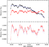 |
Fig. 1 K2 photometry of HD 80653. Top panel: light curve extracted from the MAST raw images (black dots), second-order polynomial fit of the long-term instrumental trend (blue line), corrected light-curve (red dots). Bottom panel: corrected data (red dots) with highlighted measurements obtained during transits (blue dots). Low-frequency flux variations due to the rotational modulation of photospheric active regions are clearly visible. |
2.2 HARPS-N spectroscopy
The results obtained from the analysis of the K2 photometry prompted us to include HD 80653 in our HARPS-N Collaboration’s Guaranteed Time Observations (GTO) program with the goal of precisely determining the mass of the planet. We collected 115 spectra from November 2018 to May 2019 with the HARPS-N spectrograph (R = 115 000) installed on the 3.6-m Telescopio Nazionale Galileo (TNG), located at the Observatorio del Roque de los Muchachos in La Palma, Spain (Cosentino et al. 2012).
The spectra were reduced with the version 3.8 of the HARPS-N Data Reduction Software (DRS), which includes corrections for color systematics introduced by variations in observing conditions (Cosentino et al. 2014). A numerical weighted G2 mask was used to calculate the weighted cross correlation function (CCF; Pepe et al. 2002). The DRS also provides some activity indicators, such as the full width athalf maximum (FWHM) of the CCF, the line bisector inverse slope (BIS) of the CCF, and the Mount Wilson S-index (SMW). We acquiredsimultaneous Fabry-Perot calibration spectra to correct for the instrumental drift.
All the spectra were taken with an exposure time of 900 s. Due to the short orbital period, we took between 2 and 4 spectra per night on several nights. Seven spectra with low signal-to-noise ratio (S/N) taken on two nights were no longer considered. The 108 remaining spectra have S/N in the range 40–127 (median S∕N = 84) at 550 nm.
The time series of the RVs and activity indicators are shown in Fig. 2. Error bars on the FWHM and BIS values have been taken as twice those of the RV ones (Santerne et al. 2018). A positive trend is clearly visible for the RVs, with no counterparts in the stellar activity indicators, pointing out the presence of an outer companion. We investigate this possibility in Sect. 5.
We performed a frequency analysis of the RV time series using both the generalized Lomb-Scargle periodogram (GLS; Zechmeister & Kürster 2009). and the Iterative Sine-Wave method (ISW; Vaníček 1971). The latter allowed us to remove the effects of the prewhitening by recomputing the amplitudes of the frequencies and trends previously identified (indicated as known constituents) for each new trial frequency. As expected, the long-term trend is the most prominent feature (Fig. 3, top panel). Since it is unconstrained by the time span of the observations, its value is practically 0.0 d−1 and the peak structure is very similar to the spectral window (insert in the top panel). The alias structure centered at the orbital frequency f = 1.40 d−1 is already discernible in the first power spectrum and becomes very evident when a quadratic term is introduced in the frequency analysis (bottom panel). A linear term leaves residual power close to 0.0 d−1, evidence of an unsatisfactory fit. Note that the aliases are as high as the true peak (see again the spectral window). Indeed, even if we performed more than one measurement per night, the time separation was not very large due to the high number of nights with the star visible only in the second half of the night. This did not allow the effective damping of the ±1 d−1 aliases.
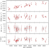 |
Fig. 2 Radial velocities and stellar activity indicators time series extracted from HARPS-N spectra. A long-term trend is a strong feature in the RV time series, but no counterpart is visible in the indicators. |
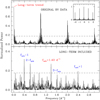 |
Fig. 3 ISW power spectra of the HARPS-N radial velocity data. The horizontal line marks FAP = 1%. Top panel: the long-term trend is the main feature in the original data. The insert shows the spectral window of the data. Bottom panel: the orbital frequency of HD 80653 b is clearly detected when a quadratic trend is added as a known constituent. |
Known stellar parameters of HD 80653.
3 Stellar modeling
Table 1 lists the known stellar parameters of HD 80653, used in the following analyses. The adopted value for the distance is discussed in Sect. 3.2.
HD 80653 atmospheric parameters. ARES+MOOG errors inflated for systematics.
3.1 Atmospheric parameters
We used three different methods to determine the stellar atmospheric parameters. The first method, CCFpams1, is based on the empirical calibration of temperature, gravity and metallicity on the equivalent width of CCFs obtained with selected subsets of stellar lines, according to their sensitivity to temperature (Malavolta et al. 2017). We obtained Teff = 5947 ± 33 K, log g = 4.41 ± 0.06 dex (cgs units), and [Fe/H] = 0.30 ± 0.03 dex.
ARES+MOOG, the second method we used, is based on the measurement of the equivalent widths of a set of iron lines. For more details, we refer the reader to Sousa (2014) and references therein. We added all HARPS-N spectra together for this analysis. Equivalent widths were automatically measured using ARESv2 (Sousa et al. 2015). The linelist comprises of roughly 300 neutral and ionised iron lines (Sousa et al. 2011). Using a grid of ATLAS plane-parallel model atmospheres (Kurucz 1993), the 2017 version of the MOOG code2 (Sneden 1973) and assuming local thermodynamic equilibrium, we determined the atmospheric parameters by imposing excitation and ionisation balance. Following the recipe from Mortier et al. (2014), we corrected the surface gravity based on the effective temperature to obtain a more accurate value. Systematic errors were added quadratically to our internal errors (Sousa et al. 2011). We obtained Teff = 6022 ± 72 K, log g = 4.36 ± 0.12 dex and [Fe/H] = 0.35 ± 0.05 dex.
Finally, we used SPC, the Stellar Parameter Classification tool (Buchhave et al. 2014), to obtain the atmospheric parameters. SPC was run on the individual RV-shifted spectra after which the values of the atmospheric parameters were averaged and weighted by their S/N. From this method, we obtained Teff = 5896 ± 50 K, log g = 4.35 ± 0.10 dex and [Fe/H] = 0.26 ± 0.08 dex. As SPC is a spectral synthesis method, it also measured the projected rotational velocity, v sin i = 3.5 ± 0.5 km s−1. The v sin i determinations made with the SPC tool have been shown to be very reliable for such lower rotational velocities (Torres et al. 2012). Table 2 summarizes the parameters determined with the different tools.
3.2 Massand radius
We determined the stellar mass and radius by fitting stellar isochrones using the adopted atmospheric parameters (Sect. 3.1), the apparent B and V magnitudes, photometry from the Two Micron All Sky Survey (2MASS; Cutri et al. 2003; Skrutskie et al. 2006) and the Wide-field Infrared Survey Explorer (WISE: Wright et al. 2010). For the atmospheric parameters, we assumed  K, σlog g= 0.12 dex and σ[Fe/H] = 0.08 dex as realistic errors for all our parameter estimates, based on the combination of the expected systematic errors (e.g. Sousa et al. 2011)and the most conservative internal error estimate for each parameter from all the techniques.
We used the code isochrones (Morton 2015) to obtain our stellar parameters. The evolutionary models are both the MESA isochrones and Stellar Tracks (MIST; Paxton et al. 2011; Choi et al. 2016; Dotter 2016) and the Dartmouth Stellar Evolution Database (Dotter et al. 2008). We ran a fit for each set of stellar atmospheric parameters and repeated the analysis for each set of stellar evolutionary models, for a total of six different fits.
As a final step, we joined the six posterior distributions from the individual fits and calculated the median and 16th and 84th percentile of the combined posterior distribution (e.g., Rice et al. 2019). We obtained consistent values within errors by using the distance values given by the Gaia DR2 parallax (Gaia Collaboration 2016, 2018), by correcting it for a systematic bias (Stassun & Torres 2018) and for the nonlinearity of the parallax-distance transformation and the asymmetry of the probability distribution (Bailer-Jones et al. 2018). We used the latter value (Table 1), intermediate between the three, to conclude that HD 80653 has a mass M⋆ = 1.18 ± 0.04 M⊙, a radius of R⋆ = 1.22 ± 0.01 R⊙ and an age of 2.7 ± 1.2 Gyr (Table 3). Note the excellent agreement between the Gaia and spectroscopic values of log g (Tables 2 and 3).
HD 80653 stellar parameters from isochrone fits as obtained from the joined posteriors of six individual fits.
3.3 Stellar activity
The light curve of HD 80653 (Fig. 1) clearly shows modulated rotational cycles due to active regions on the stellar surface, with clearly evident cycle-to-cycle variations. In particular, we note that the standstill at the level of the average flux around BJD 2458145 seems to strongly modify the shape of the light curve. To investigate this, we firstly removed the in-transit measurements and then we performed the frequency analysis on the whole dataset and then on two subsets: the first composed of the measurements before BJD 2458145 and the second composed of those after BJD 2458145. The resulting GLS power spectra are shown in Fig 4. They suggest a rotational modulation with frot = 0.055 d−1 and harmonics in the first subset and frot = 0.037 d−1 and harmonics in the second subset. The presence of harmonics indicates a double-wave shape over the rotational period. This suggests that the star is seen nearly equator-on with activity in both hemispheres. The frequencies correspond to Prot = 18 d and 27 d, respectively, but the latter value is poorly constrained due to the short time coverage. The power spectrum of the full data set does not supply useful hints, since several peaks appear as the mergingof the incoherent frequencies detected in the two subsets. We can conjecture that in the two time intervals two small spots (or groups) appear on well separated regions of the stellar surface.
The measured v sin i (Table 2) and inferred stellar radius (Table 3) result in a maximum rotation period Prot = 18 ± 3 d. This is in excellent agreement with the value of the first subset, while that of the second subset is too long. Therefore, it is probable that such a long period is spurious due to the simultaneous visibility of several spots widely distributed in longitude. Taking into account that the flux variability of HD 80653 is very small (~0.1%), the appearance of small spots can easily alter the light curve. The scenario becomes still more complicated if the spots are also in differential rotation.
We also investigated the periodicities in the spectroscopic time series. Firstly, we reanalyzed the RV data by including the long-term trend and the orbital frequency as known constituents. No clear peak suggesting other planetary signals was detected (Fig. 5, top panel). Then we analyzed the main activity indicators FWHM, BIS, and SMW. We immediately noted that none of the periodograms of these indicators show a peak at the frequency f =1.40 d−1 detected in the RV data (Fig. 5, other panels), definitely supporting its full identification as the orbital frequency of HD 80653 b. This absence also suggests a weak star-to-planet interaction, if any. On the other hand, these periodograms show some peaks in the frequency range where we found signals in the K2 photometry, namely, 0.03–0.06 d−1 (the grey region). In particular, the SMW data and the RV residuals show peaks above the FAP = 1% threshold at f = 0.060 d−1, that is, P = 16.6 d. Therefore K2 photometry, v sin i measurement, and activity indicators all suggest a stellar rotation period in the range 16–20 d.
Finally, we calculated the Spearman correlation coefficients for the original RV versus FWHM, BIS, and SMW weighted values (Fig. 6). We obtained 0.355, − 0.014, and 0.378, respectively.
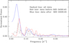 |
Fig. 4 GLS power spectra of the K2 data. The full data set has been subdivided into two subsets, before and after BJD 2458145. Two different rotational frequencies are then detected. The power spectrum of the full data set appears as an average of the two. |
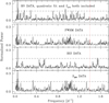 |
Fig. 5 Top to bottom: ISW power spectra of the RV (long-term trend and orbital frequency considered as known constituents), FWHM, BIS, SMW (no known constituent) timeseries. The vertical red line indicates the orbital period of the transiting planet. The grey region at low frequencies delimits the interval where the rotational frequency is expected from the K2 photometry. The horizontal lines mark the 1% FAP. |
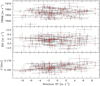 |
Fig. 6 RVs versus activity indicators FWHM, BIS, and SMW. |
4 Photometric modeling
The planetary transits are clearly detected in the K2 light curve, both when extracted from the raw images (top panel of Fig. 1) and after correction for the instrumental drift (bottom panel). This is thanks to the limited variability (~0.1%) of HD 80653 and to the sharpness of the planetary transits. Moreover, due to the ultra-short orbital period, the transits have been observed at almost all the stellar activity levels, thus making very effective the cancellation of the effects produced by unocculted small spots and faculae. Therefore, we were able to perform a very reliable analyses both for the transit and the occultation of the exoplanet.
4.1 Primary transit
We performed the transit fit using PyORBIT (Malavolta et al. 2016, 2018). We assumed a circular orbit for the planet, applying a parametrisation for the limb darkening (Kipping 2013) and imposing a prior on the stellar density directly derived from the posterior distributions of M⋆ and R⋆. We note that a Keplerian fit with no assumption on the eccentricity returned a value consistent with zero.
We removed stellar variability from the K2 light curve by dividing away the best-fit spline from our simultaneous systematics fit described in Sect. 2.1, and used this flattened light curve in our transit-fit analysis. PyORBIT relies on the batman code (Kreidberg 2015) to model the transit, with an oversampling factor of 10 when accounting for the 1764.944 s exposure time of the K2 observations (Kipping 2010). Posterior sampling was performed with an affine-invariant Markov chain Monte Carlo (MCMC) emcee sampler (Foreman-Mackey et al. 2013), with starting points for the chains obtained from the global optimization code PyDE3. We ran the sampler for 50 000 steps, discarding the first 15 000 steps as a conservative burn-in.
We obtained an orbital period Pb = 0.719573 ± 0.000021 d and a reference central time of transit Tc = 2 458 134.4244 ± 0.0007 BJD. The stellar density as derived from the transit fit agrees with that determined in Sect. 3.2 (Table 3). The planetary radius is therefore Rb = 1.613 ± 0.071 R⊕, given the stellar radius presented in Sect. 3. We also ran a fit using the raw light curve and modelling it with a Gaussian Process through the celerite package (Foreman-Mackey et al. 2017). The results were perfectly consistent with the results from the pre-flattened light curve. All parameters are reported in Table 4 and the phase-folded light curve with the best fit is shown in Fig. 7. We also measured a much lower value of the K2 correlated noise (14 ppm) than that of the photometric errors (60 ppm). The procedures to compute them are described in Pont et al. (2006) and Bonomo et al. (2012). The resulting total noise is then 62 ppm.
The values of v sin i, transit depth and impact parameter provide an expected semi-amplitude of 47 ± 10 cm s−1 for the Rossiter-McLaughlin effect. This amplitude is smaller than our σRV errors.
HD 80653 system parameters.
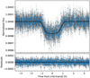 |
Fig. 7 Top: HD 80653 b transit light curve phase-folded to a period of Pb = 0.719573 d, as determined using PyORBIT. Bottom: residuals of the transit fit. |
4.2 Secondary eclipse and phase curve
For a few USP planets, namely Kepler-10b (Batalha et al. 2011), Kepler-78b (Sanchis-Ojeda et al. 2013) and K2-141b (Malavolta et al. 2018), Kepler data have also allowed us to detect the optical secondary eclipse and the flux variations along the orbital phase4. Assuming that the secondary eclipse is mainly due to the planet’s thermal emission in the Kepler bandpass for the high day-side temperature, the comparison between the depth of the secondary eclipse, δec, and the amplitude of the flux variations along the phase, Aill, may providesome constraints on the nature of the USP planets.
To search for the secondary eclipse and flux variations along the phase in HD 80653, we removed the stellar variability in the K2 flux curve using the same method as in Sanchis-Ojeda et al. (2013). In the resulting filtered flux curve, we simultaneously modeled the primary transit, the secondary eclipse, and the flux variations along the phase by assuming a circular orbit and by using the modified model of Mandel & Agol (2002) without limb darkening for the secondary eclipse, and the prescriptions in Esteves et al. (2013) for the flux variations along the phase. Doppler boosting and ellipsoidal variations are negligible and hence were not incorporated in our model. The model was created with a 1-min time sampling and then binned to the long cadence sampling of the K2 data points. We imposed a Gaussian prior on the stellar density (Table 3) and fixed the quadratic limb-darkening coefficients to the values previously found (Sect. 4.1 and Table 4). We employed a differential evolution MCMC technique (DE-MCMC; Ter Braak 2006) as implemented in the ExofastV2 code (Eastman et al. 2013; Eastman 2017) to derive the posterior distributions of the fitted parameters (Fig. A.1).
The values and uncertainties of the primary transit parameters are fully consistent with those determined in Sect. 4.1. Our procedure pointed out a possible secondary eclipse with a depth of δec = 8.1 ± 3.7 ppm at 0.50 Pb (Fig. 8). We computed the values of the Bayesian Information Criterion (BIC; Liddle 2007) for the two models with and without the secondary eclipse. We obtained ΔBIC = 5.2 and hence a Bayes factor B10 ~ 13.5 in favor of the former (Burnham & Anderson 2004). By using appropriate guidelines (see Sect. 3.2 in Kass & Raftery 1995), this value provides a positive evidence for the detection of the secondary eclipse. Due to the large relative uncertainty on the occultation depth, the threshold for a strong detection (B10 = 20) could not be reached.
The flux variations along the phase are not detected since their amplitude is consistent with zero: Aill = 2.7 ± 3.5 ppm. Despite the large uncertainty on δec, we estimated the planet geometric albedo as a function of the day-side temperature (Fig. 9). Since the planet is highly irradiated, the most important contribution to the secondary eclipse depth might come from the day-side thermal emission rather than the light reflected by the planet surface. Figure 9 shows that the maximum achievable day-side temperature could be  K for a null Bond albedo. Theoretical computations for a null Bond albedo and an efficient heat circulation predict a maximum night-side temperature
  K.
K.
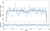 |
Fig. 8 Phase-folded secondary eclipse with the best-fit model and the residuals at the bottom. The data has been binned by a factor of 100 for clarity. |
5 Radial velocity modeling
We used two different methods to model the RVs. In both methods we assumed a circular orbit. This assumption is mainly based on the extremely short circularization time for such a close-in planet, that is, < 0.5 Myr (Matsumura et al. 2008), computed from a modified tidal quality factor similar to that of the Earth ( ), which is reasonable given the rocky composition of HD 80653 b (Table 4 and Sect. 6).
In the first method we computed the planetary RVs relative to nightly offsets. This was possible since the orbital period is much shorter than the rotational period. We modeled the planetary signal fitting for nightly offset values calculated every two orbital periods, using the formula
![Mathematical equation: \[ \textrm{RV} = K\sin{\left(\frac{2\pi}{P} x(t)\right)} + \sum_{i\,=\,0}^{N}B_i\Theta(t-t_0 - 2iP),\vspace*{-3pt} \]](/articles/aa/full_html/2020/01/aa36689-19/aa36689-19-eq5.png)
where P is the orbital period determined from the light curve, Θ(t) is the Heaviside step function, t0 is the time of the first HARPS-N RV measurement, N is the number of nightly offsets, and x(t) is the phase-folded mid-exposure time. We find the best-fit parameters via simple likelihood estimate (i.e., χ2), and then use an MCMC technique (as implemented in python by emcee; Foreman-Mackey et al. 2013) to determine appropriate errors on the RV amplitude and RV offsets, K and {Bi} respectively, while P and Tc are determined from the photometric analysis and are thus held constant. We use flat, non-informative priors for all values and 700 walkers taking 600 steps. The walkers are initially placed in a small sphere (or Gaussian ball) around the values of the Maximum Likelihood Estimate parameters. The first 50 samples are removed as burn-in, and we then marginalize over all Bi s to obtain the posterior distribution for K; the width of this distribution gives us the errors on the RV amplitude. We obtained an RV semi-amplitude of K = 3.46 ± 0.27 m s−1 due to planet b, corresponding to a mass Mb = 5.5 ± 0.5M⊕, and a density ρb = 7.2 ± 1.1 g cm−3.
In the second method we used PyORBIT to simultaneously model an orbit for the planetary signal and a polynomial to account for the trend in the RV data (Fig. 2). We imposed Gaussian priors based on the light-curve fit on Porb and Tc (Sect. 4). A first attempt at fitting the data without any modelling of the stellar activity resulted in a RV jitter of 2.9 ± 0.3 m s−1, clearly indicating the presence of an additional signal in the data. We then included in our analysis a Gaussian Process (GP) trained on both the SMW index and FWHM, since these indicators show hints of rotational modulation (Sect. 3.3). We used a quasi-periodic kernel with independent amplitudes of covariance function h for each dataset, but with the rotational period Prot, coherence scale w, and decay timescale of activity regions λ in common. We used the george library (Ambikasaran et al. 2015) to implement the mathematical definition of the kernel given by Grunblatt et al. (2015). We constrained w to  as suggested by López-Morales et al. (2016), but taking care to recompute the proposed prior of
  to take into account the different coefficients in the kernel definition. Non-informative, uniform priors with broad intervals were used for all the other parameters. Posterior sampling and confidence intervals were obtained following the same procedure described in Sect. 4.
We obtained very consistent results from the GPs trained firstly on the SMW indicator and then on the FWHM one. Both match very well the photometric determination of the rotational period, namely, Prot = 19.2 d. We report the confidence intervals relative to the approach using the FWHM index (Table 4). We emphasize that the posterior distributions of the planet’s parameters were not affected by the exact choices for the GP regression. Indeed, for sake of completeness, we repeated the analysis using the RV data alone, obtaining again similar results, but larger errors. The GP analysis yielded an RV semi-amplitude of K = 3.55 ± 0.26 m s−1 for the planet b, corresponding to a mass Mb= 5.60 ± 0.43M⊕ after taking into account the error on the period, stellar mass and the orbital inclination.
The two methods used to model the RVs yield consistent results on the RV semi-amplitude and planetary mass. The parameters obtained with PyORBIT (Table 4) were used to continue our analysis. The resulting RV values with the best-fit model are shown in Fig. 10.
For sake of completeness, we performed the PyORBIT analysis not assuming a circular orbit. It returned an eccentricity value consistent with zero and parameters all consistent with the circular case. We also repeated the analysis described above to search for another short-period planet in the system, in a circular or eccentric orbit, but we did not detect any clear signal.
The long-term trend seen in the RV plot only (Fig. 2) strongly suggests an additional Keplerian motion, since long-term activity cycles should show analogues in the specific indicators and HARPS-N has a proven long-term instrumental stability. The steady increase ( = 0.17 m s−1d−1) spans about 150 days. There is a relation between
  and some properties of the companion (Winn et al. 2009)
![Mathematical equation: \[ \frac{m_{\textrm{c}} \sin{i_{\textrm{c}}}}{a_{\textrm{c}}^{2}} \sim \frac{\dot{\gamma}}{G} = (0.37 \pm 0.08)\,{M_{\textrm{Jup}} \,\textrm{AU}}^{-2}, \]](/articles/aa/full_html/2020/01/aa36689-19/aa36689-19-eq11.png)
where mc is the companion mass, ic its orbital inclination relative to the line ofsight, and ac its orbital distance. Assuming i ≃ 90o, a substellar companion of 15 MJup would orbit at 6.4 AU, with a period of 5500 d. However, the last RV measurements seem to suggest a possible curvature, as noted in the frequency analysis (Sect. 2.2). In such a case, and assuming a moderate eccentricity, we can estimate a period in the range 260−400 d and a RV amplitude 2Kc ≃ 25 m s−1. Under these hypothetical conditions, we can tentatively suggest a mass of 0.35−0.50 MJup for the companion. The only way to solve the ambiguities on its presence and location is to continue monitoring the system in future observing seasons.
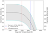 |
Fig. 9 Geometric albedo vs day-side temperature. The dashed lines correspond to the maximum planet day-side temperature (black), the equilibrium temperature in the no-albedo and no-circulation limit (blue) and the uniform temperature for a null Bond albedo and extreme heat circulation (red). The shaded grey region displays the 1σ interval for the geometric albedo. |
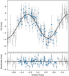 |
Fig. 10 Top panel: phase-folded RV fit obtained using PyORBIT. Activity jitter and long-term trend both removed. Larger blue dots delimitate the RV variation over a single orbital cycle. Bottom panel: residuals from the best fit. |
6 Discussion and conclusions
We used K2 photometry and high-resolution spectroscopy to determine the HD 80653 system parameters and, in particular, the mass and density of its USP transiting planet. A combined analysis of the high-precision HARPS-N RVs and the K2 data reveals that this planet has an orbital period Pb = 0.719573 ± 0.000021 d, a radius Rb = 1.613 ± 0.071 R⊕, and a mass Mb = 5.60 ± 0.43 M⊕. Its density is then ρb = 7.4 ± 1.1 g cm−3.
Figure 11 shows the mass-radius diagram for all small planets (Rp< 2.8 R⊕) with a mass determined with a precision better than 30%5. HD 80653 b has a bulk density consistent, within uncertainties, with that of an Earth-like rocky composition (32.5% Fe/Ni-metal+ 67.5% Mg-silicates-rock). Owing to its proximity to the host star (1/60 AU), 1Gand the host star being brighter than our own Sun (a factor of 1.67 times the bolometric luminosity of the Sun), HD 80653 b receives very high bolometric irradiation (radiation flux received per unit surface area is about 6000 times the insolation at the Earth’s surface). Thus, its equilibrium surface temperature for null albedo and uniform redistribution Tunif of heat to the night-side is on the order of 2500 K, enough to completely melt most silicates-rocky materials as well as iron and its alloys under 1-bar surface pressure. Therefore, it is expected to be a lava-ocean world, especially at the substellar point facing the star. The uncertainty in our mass determination is small enough that our density estimate excludes the presence of any significant envelope of volatiles or H/He on the surface of the planet.
Other similar exoplanets can provide useful information about the physical conditions on the surface of HD 80653 b. 55 Cnc e is a super-Earth orbiting a sun-like star in 0.7 d (Crida et al. 2018). Spitzer infrared observations (Demory et al. 2016)show that 55 Cnc e is tidally-locked to the host star, meaning that one hemisphere of the planet always faces the host star, with a hot spot phase-shifted eastward of the substellar point by about 40 degrees. Furthermore, the 4.5 μm phase curveshows that there is a significant temperature difference, on the order of ~1000 K, between theday-side and night-side of the planet. Under the intense stellar irradiation on the day-side, which results in the estimated high temperature, there is likely a hemispherical silicate-vapor atmosphere developed on top of the molten liquid silicates (magma pool; Kite et al. 2016). This silicate-vapor atmosphere would include gaseous species such as SiO and Na (Schaefer & Fegley 2009). On the other hand, LHS 3844 b is a 1.3 R⊕ world orbiting a small-size, low-mass and cool star (R⋆ = 0.18 R⊙, M = 0.16 M⊙, and Teff = 3036 K) in 0.46 d. Ithas been modeled as a bare-rock planet, with no atmosphere, but unfortunately we do not know the mass (Kreidberg et al. 2019). Spitzer light curve shows symmetric, large amplitude flux variations along the orbital phase, implying a day-side T =1040 K and a night-side close to 0 K.
In the case of HD 80653, assuming that both the depth of the secondary eclipse (8.1 ± 3.7 ppm) and the flux variations along the phase (consistent with zero) are due to the planet’s thermal light, this might indicate non-negligible night-side emission, which would be at odds with the lava-ocean planet model (Léger et al. 2011) predicting inefficient circulation. Two reasons prevent us from drawing any firm conclusion: (i) the large uncertainties on the amplitudes of the secondary eclipse and of the flux variations along the phase, (ii) the well-known degeneracy between reflected and thermal light in the Kepler optical bandpass (Cowan & Agol 2011). Precise space-based photometry (e.g., JWST, CHEOPS) would be extremely useful to unveil the nature of the USP super-Earth HD 80653 b.
We may also consider the process by which HD 80653 b formed. It is unlikely that such an USP planet could form in situ, because a simple equilibrium condensation calculation shows that Magnesium-Silicates, one of the major chemical components of rocks, would only condense out of the nebula from gas phase into solid phase below around 1400 K (Lewis 2004). It is more likely that it initially formed on a wider orbit and was subsequently transported to its current proximity to the star through migration.
In such a scenario the unseen companion could play a relevant role. Indeed, HD 80653 exhibits a long-term RV trend, with possible hints of curvature towards the end of the observing period. This is suggestive of the existence of an outer, more massive companion. Continued RV monitoring of the system, significantly extending the present time baseline, would enable tight constraints on its orbital parameters and mass, thereby allowing investigations of its role in the formation of the USP super-Earth HD 80653 b. Given that HD 80653 is bright, and in proximity of the Sun, intermediate-separation giant planetary and brown dwarf companions are likely to be detectable using Gaia (e.g., Sozzetti & de Bruijne 2018, and references therein). In less than two years time, the third major Gaia Data Release, based on about three years of data collection, might allow us to place an additional, independent constraint on the orbital architecture of the HD 80653 planetary system.
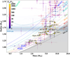 |
Fig. 11 Mass-radius diagram of planets smaller than ~2.8 R⊕. The data points are shaded according to the precision on the mass, with a full color indicating a value better than 20%. Earth and Venus are shown for comparison. The dashed lines show planetary interior models for different compositions as labelled (Zeng et al. 2019). Planets are color-coded according to the incident flux Fp, relative to the solar constant F⊙ The horizontal light-blue shade centered on R ~ 1.70 R⊕ shows the radius Gap. The shaded gray region marks the maximum value of iron content predicted by collisional stripping (Marcus et al. 2010). |
Acknowledgements
The HARPS-N project has been funded by the Prodex Program of the Swiss Space Office (SSO), the Harvard University Origins of Life Initiative (HUOLI), the Scottish Universities Physics Alliance (SUPA), the University of Geneva, the Smithsonian Astrophysical Observatory (SAO), and the Italian National Astrophysical Institute (INAF), the University of St Andrews, Queen’s University Belfast, and the University of Edinburgh. Based on observations made with the Italian Telescopio Nazionale Galileo (TNG) operated by the Fundación Galileo Galilei (FGG) of the Istituto Nazionale di Astrofisica (INAF) at the Observatorio del Roque de los Muchachos (La Palma, Canary Islands, Spain). G.F. acknowlwdges support from the INAF/FRONTIERA project through the “Progetti Premiali” funding scheme of the Italian Ministry of Education, University, and Research. A.M. acknowledges support from the senior Kavli Institute Fellowships. A.C.C. acknowledges support from the Science and Technology Facilities Council (STFC) consolidatedgrant number ST/R000824/1 and UKSA grant ST/R003203/1. F.P. kindly acknowledges the Swiss National Science Foundation for its continuous support to the HARPS-N GTO programme through the grants Nr. 184618, 166227 and 200020_152721. R.D.H. and A.V performed this work under contract with the California Institute of Technology (Caltech)/Jet Propulsion Laboratory (JPL) funded by NASA through the Sagan Fellowship Program executed by the NASA Exoplanet Science Institute. This research has made use of the SIMBAD database, operated at CDS, Strasbourg, France, and NASA’s Astrophysics Data System. This research has made use of the NASA Exoplanet Archive, which is operated by the California Institute of Technology, under contract with the National Aeronautics and Space Administration under the Exoplanet Exploration Program. This material is based upon work supported by the National Aeronautics and Space Administration under grant No. NNX17AB59G issued through the Exoplanets Research Program. This work has made use of data from the European Space Agency (ESA) mission Gaia (https://www.cosmos.esa.int/gaia), processed by the Gaia Data Processing and Analysis Consortium (DPAC, https://www.cosmos.esa.int/web/gaia/dpac/consortium). Funding for the DPAC has been provided by national institutions, in particular the institutions participating in the Gaia Multilateral Agreement. This paper includes data collected by the K2 mission. Funding for the K2 mission is provided by the NASA Science Mission directorate. Some of the data presented in this paper were obtained from the Mikulski Archive for Space Telescopes (MAST). STScI is operated by the Association of Universities for Research in Astronomy, Inc., under NASA contract NAS5-26555. Support for MAST for non-HST data is provided by the NASA Office of Space Science via grant NNX13AC07G and by other grants and contracts.
Appendix A Additional figure
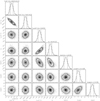 |
Fig. A.1 Posterior distributions of the best-fit DE-MCMC parameters estimating a secondary eclipse of 8 ± 4 ppm and flux variations along the phase consistent with zero within 1σ. |
References
- Ambikasaran, S., Foreman-Mackey, D., Greengard, L., Hogg, D. W., & O’Neil, M. 2015, IEEE Trans. Pattern Anal. Mach. Intell., 38, 252 [NASA ADS] [CrossRef] [Google Scholar]
- Bailer-Jones, C. A. L., Rybizki, J., Fouesneau, M., Mantelet, G., & Andrae, R. 2018, AJ, 156, 58 [NASA ADS] [CrossRef] [Google Scholar]
- Batalha, N. M., Borucki, W. J., Bryson, S. T., et al. 2011, ApJ, 729, 27 [NASA ADS] [CrossRef] [Google Scholar]
- Bonomo, A. S., Chabaud, P. Y., Deleuil, M., et al. 2012, A&A, 547, A110 [NASA ADS] [CrossRef] [EDP Sciences] [Google Scholar]
- Buchhave, L. A., Bizzarro, M., Latham, D. W., et al. 2014, Nature, 509, 593 [NASA ADS] [CrossRef] [Google Scholar]
- Burnham, K. P., & Anderson, D. R. 2004, Sociol. Methods Res., 33, 261 [Google Scholar]
- Chiang, E., & Laughlin, G. 2013, MNRAS, 431, 3444 [Google Scholar]
- Choi, J., Dotter, A., Conroy, C., et al. 2016, ApJ, 823, 102 [NASA ADS] [CrossRef] [Google Scholar]
- Cosentino, R., Lovis, C., Pepe, F., et al. 2012, SPIE Conf. Ser., 8446, 84461V [Google Scholar]
- Cosentino, R., Lovis, C., Pepe, F., et al. 2014, SPIE Conf. Ser., 9147, 91478C [Google Scholar]
- Cowan, N. B., & Agol, E. 2011, ApJ, 729, 54 [NASA ADS] [CrossRef] [Google Scholar]
- Crida, A., Ligi, R., Dorn, C., & Lebreton, Y. 2018, ApJ, 860, 122 [NASA ADS] [CrossRef] [Google Scholar]
- Cutri, R. M., Skrutskie, M. F., van Dyk, S., et al. 2003, VizieR Online Data Catalog: II/246 [Google Scholar]
- Demory, B.-O., Gillon, M., de Wit, J., et al. 2016, Nature, 532, 207 [NASA ADS] [CrossRef] [Google Scholar]
- Dotter, A. 2016, ApJS, 222, 8 [NASA ADS] [CrossRef] [Google Scholar]
- Dotter, A., Chaboyer, B., Jevremović, D., et al. 2008, ApJS, 178, 89 [NASA ADS] [CrossRef] [Google Scholar]
- Eastman, J. 2017, EXOFASTv2: Generalized publication-quality exoplanet modeling code [Google Scholar]
- Eastman, J., Gaudi, B. S., & Agol, E. 2013, PASP, 125, 83 [NASA ADS] [CrossRef] [Google Scholar]
- Ehrenreich, D., Bourrier, V., Wheatley, P. J., et al. 2015, Nature, 522, 459 [Google Scholar]
- Esteves, L. J., De Mooij, E. J. W., & Jayawardhana, R. 2013, ApJ, 772, 51 [NASA ADS] [CrossRef] [Google Scholar]
- Foreman-Mackey, D., Hogg, D. W., Lang, D., & Goodman, J. 2013, PASP, 125, 306 [CrossRef] [Google Scholar]
- Foreman-Mackey, D., Agol, E., Ambikasaran, S., & Angus, R. 2017, AJ, 154, 220 [NASA ADS] [CrossRef] [Google Scholar]
- Fulton, B. J., & Petigura, E. A. 2018, AJ, 156, 264 [NASA ADS] [CrossRef] [Google Scholar]
- Fulton, B. J., Petigura, E. A., Howard, A. W., et al. 2017, AJ, 154, 109 [NASA ADS] [CrossRef] [Google Scholar]
- Gaia Collaboration (Prusti, T., et al.) 2016, A&A, 595, A1 [NASA ADS] [CrossRef] [EDP Sciences] [Google Scholar]
- Gaia Collaboration (Brown, A. G. A., et al.) 2018, A&A, 616, A1 [NASA ADS] [CrossRef] [EDP Sciences] [Google Scholar]
- Grunblatt, S. K., Howard, A. W., & Haywood, R. D. 2015, ApJ, 808, 127 [NASA ADS] [CrossRef] [Google Scholar]
- Howard, A. W., Marcy, G. W., Bryson, S. T., et al. 2012, ApJS, 201, 15 [NASA ADS] [CrossRef] [Google Scholar]
- Kass, R. E., & Raftery, A. E. 1995, J. Am. Stat. Assoc., 90, 773 [Google Scholar]
- Kipping, D. M. 2010, MNRAS, 408, 1758 [NASA ADS] [CrossRef] [Google Scholar]
- Kipping, D. M. 2013, MNRAS, 435, 2152 [Google Scholar]
- Kite, E. S., Fegley, Jr. B., Schaefer, L., & Gaidos, E. 2016, ApJ, 828, 80 [NASA ADS] [CrossRef] [Google Scholar]
- Kovács, G., Zucker, S., & Mazeh, T. 2002, A&A, 391, 369 [NASA ADS] [CrossRef] [EDP Sciences] [Google Scholar]
- Kreidberg, L. 2015, PASP, 127, 1161 [NASA ADS] [CrossRef] [Google Scholar]
- Kreidberg, L., Koll, D. D. B., Morley, C., et al. 2019, Nature, 573, 87 [NASA ADS] [CrossRef] [Google Scholar]
- Kurucz, R. L. 1993, SYNTHE Spectrum Synthesis Programs and Line Data (Cambridge, MA: Smithsonian Astrophysical Observatory) [Google Scholar]
- Lee, E. J., & Chiang, E. 2017, ApJ, 842, 40 [NASA ADS] [CrossRef] [Google Scholar]
- Léger, A., Grasset, O., Fegley, B., et al. 2011, Icarus, 213, 1 [NASA ADS] [CrossRef] [Google Scholar]
- Lewis, J. S. 2004, Physics and Chemistry of the Solar System (Cambridge, MA: Elsevier Academic Press), 655 [Google Scholar]
- Liddle, A. R. 2007, MNRAS, 377, L74 [NASA ADS] [Google Scholar]
- Lopez, E. D., & Fortney, J. J. 2013, ApJ, 776, 2 [NASA ADS] [CrossRef] [Google Scholar]
- López-Morales, M., Haywood, R. D., Coughlin, J. L., et al. 2016, AJ, 152, 204 [NASA ADS] [CrossRef] [Google Scholar]
- Lundkvist, M. S., Kjeldsen, H., Albrecht, S., et al. 2016, Nat. Commun., 7, 11201 [Google Scholar]
- Malavolta, L., Nascimbeni, V., Piotto, G., et al. 2016, A&A, 588, A118 [NASA ADS] [CrossRef] [EDP Sciences] [Google Scholar]
- Malavolta, L., Lovis, C., Pepe, F., Sneden, C., & Udry, S. 2017, MNRAS, 469, 3965 [NASA ADS] [CrossRef] [Google Scholar]
- Malavolta, L., Mayo, A. W., Louden, T., et al. 2018, AJ, 155, 107 [NASA ADS] [CrossRef] [Google Scholar]
- Mandel, K., & Agol, E. 2002, ApJ, 580, L171 [NASA ADS] [CrossRef] [Google Scholar]
- Marcus, R. A., Sasselov, D., Hernquist, L., & Stewart, S. T. 2010, ApJ, 712, L73 [NASA ADS] [CrossRef] [Google Scholar]
- Matsumura, S., Takeda, G., & Rasio, F. A. 2008, ApJ, 686, L29 [NASA ADS] [CrossRef] [Google Scholar]
- Mayor, M., Marmier, M., Lovis, C., et al. 2011, ArXiv e-prints [arXiv:1109.2497] [Google Scholar]
- Mortier, A., Sousa, S. G., Adibekyan, V. Z., Brandão, I. M., & Santos, N. C. 2014, A&A, 572, A95 [NASA ADS] [CrossRef] [EDP Sciences] [Google Scholar]
- Morton, T. D. 2015, Astrophysics Source Code Library [record ascl:1503.010] [Google Scholar]
- Owen, J. E., & Wu, Y. 2013, ApJ, 775, 105 [Google Scholar]
- Owen, J. E., & Wu, Y. 2017, ApJ, 847, 29 [NASA ADS] [CrossRef] [Google Scholar]
- Paxton, B., Bildsten, L., Dotter, A., et al. 2011, ApJS, 192, 3 [Google Scholar]
- Pepe, F., Mayor, M., Rupprecht, G., et al. 2002, The Messenger, 110, 9 [NASA ADS] [Google Scholar]
- Pepe, F., Cameron, A. C., Latham, D. W., et al. 2013, Nature, 503, 377 [NASA ADS] [CrossRef] [PubMed] [Google Scholar]
- Pont, F., Zucker, S., & Queloz, D. 2006, MNRAS, 373, 231 [NASA ADS] [CrossRef] [Google Scholar]
- Queloz, D., Bouchy, F., Moutou, C., et al. 2009, A&A, 506, 303 [NASA ADS] [CrossRef] [EDP Sciences] [Google Scholar]
- Rice, K. 2015, MNRAS, 448, 1729 [NASA ADS] [CrossRef] [Google Scholar]
- Rice, K., Malavolta, L., Mayo, A., et al. 2019, MNRAS, 484, 3731 [NASA ADS] [CrossRef] [Google Scholar]
- Rogers, L. A. 2015, ApJ, 801, 41 [NASA ADS] [CrossRef] [Google Scholar]
- Sanchis-Ojeda, R., Rappaport, S., Winn, J. N., et al. 2013, ApJ, 774, 54 [NASA ADS] [CrossRef] [Google Scholar]
- Sanchis-Ojeda, R., Rappaport, S., Winn, J. N., et al. 2014, ApJ, 787, 47 [NASA ADS] [CrossRef] [Google Scholar]
- Santerne, A., Brugger, B., Armstrong, D. J., et al. 2018, Nat. Astron., 2, 393 [NASA ADS] [CrossRef] [Google Scholar]
- Schaefer, L., & Fegley, B. 2009, ApJ, 703, L113 [NASA ADS] [CrossRef] [Google Scholar]
- Schneider, J., Dedieu, C., Le Sidaner, P., Savalle, R., & Zolotukhin, I. 2011, A&A, 532, A79 [NASA ADS] [CrossRef] [EDP Sciences] [Google Scholar]
- Skrutskie, M. F., Cutri, R. M., Stiening, R., et al. 2006, AJ, 131, 1163 [NASA ADS] [CrossRef] [Google Scholar]
- Sneden, C. A. 1973, PhD Thesis, The University of Texas at Austin, Austin, USA [Google Scholar]
- Sousa, S. G. 2014, Determination of Atmospheric Parameters of B-, A-, F- and G-Type Stars (Berlin: Springer), 297 [Google Scholar]
- Sousa, S. G., Santos, N. C., Israelian, G., et al. 2011, A&A, 526, A99 [NASA ADS] [CrossRef] [EDP Sciences] [Google Scholar]
- Sousa, S. G., Santos, N. C., Adibekyan, V., Delgado-Mena, E., & Israelian, G. 2015, A&A, 577, A67 [NASA ADS] [CrossRef] [EDP Sciences] [Google Scholar]
- Sozzetti, A., & de Bruijne, J. 2018, Handbook of Exoplanet, Space Astrometry Missions for Exoplanet Science: Gaia and the Legacy of Hipparcos (Berlin: Springer), 81 [Google Scholar]
- Stassun, K. G., & Torres, G. 2018, ApJ, 862, 61 [NASA ADS] [CrossRef] [Google Scholar]
- Ter Braak, C. J. F. 2006, Stat. Comput., 16, 239 [Google Scholar]
- Torres, G., Fischer, D. A., Sozzetti, A., et al. 2012, ApJ, 757, 161 [NASA ADS] [CrossRef] [Google Scholar]
- Vanderburg, A., & Johnson, J. A. 2014, PASP, 126, 948 [NASA ADS] [CrossRef] [Google Scholar]
- Vanderburg, A., Latham, D. W., Buchhave, L. A., et al. 2016, ApJS, 222, 14 [NASA ADS] [CrossRef] [Google Scholar]
- Van Eylen, V., Agentoft, C., Lundkvist, M. S., et al. 2018, MNRAS, 479, 4786 [NASA ADS] [CrossRef] [Google Scholar]
- Vaníček, P. 1971, Ap&SS, 12, 10 [NASA ADS] [CrossRef] [Google Scholar]
- Winn, J. N., Johnson, J. A., Albrecht, S., et al. 2009, ApJ, 703, L99 [NASA ADS] [CrossRef] [Google Scholar]
- Winn, J. N., Sanchis-Ojeda, R., Rogers, L., et al. 2017, AJ, 154, 60 [NASA ADS] [CrossRef] [Google Scholar]
- Winn, J. N., Sanchis-Ojeda, R., & Rappaport, S. 2018, New Astron. Rev., 83, 37 [NASA ADS] [CrossRef] [Google Scholar]
- Wright, E. L., Eisenhardt, P. R. M., Mainzer, A. K., et al. 2010, AJ, 140, 1868 [NASA ADS] [CrossRef] [Google Scholar]
- Yu, L., Crossfield, I. J. M., Schlieder, J. E., et al. 2018, AJ, 156, 22 [NASA ADS] [CrossRef] [Google Scholar]
- Zechmeister, M., & Kürster, M. 2009, A&A, 496, 577 [NASA ADS] [CrossRef] [EDP Sciences] [Google Scholar]
- Zeng, L., Jacobsen, S. B., & Sasselov, D. D. 2017, Res. Notes AAS, 1, 32 [Google Scholar]
- Zeng, L., Jacobsen, S. B., Sasselov, D. D., et al. 2019, Proc. Natl. Acad. Sci., 116, 9723 [Google Scholar]
Exoplanet papers usually call these “phase variations”. However, that is misleading with regards to the originary definition used in the study of variable stars. In the latter, “phase variations” indicate variations in the phase values of periodic light-curves, e.g. ϕi in m(t) = mo + ∑iAi cos[2π i f(t − To) + ϕi], along the time. It thus defines cycle-to-cycle variations, which is not what is meant in the context of exoplanets.
Data from exoplanetarchive.ipac.caltech.edu (Exoplanet Archive) and www.exoplanet.eu (Schneider et al. 2011).
All Tables
HD 80653 stellar parameters from isochrone fits as obtained from the joined posteriors of six individual fits.
All Figures
|
Fig. 1 K2 photometry of HD 80653. Top panel: light curve extracted from the MAST raw images (black dots), second-order polynomial fit of the long-term instrumental trend (blue line), corrected light-curve (red dots). Bottom panel: corrected data (red dots) with highlighted measurements obtained during transits (blue dots). Low-frequency flux variations due to the rotational modulation of photospheric active regions are clearly visible. |
| In the text | |
|
Fig. 2 Radial velocities and stellar activity indicators time series extracted from HARPS-N spectra. A long-term trend is a strong feature in the RV time series, but no counterpart is visible in the indicators. |
| In the text | |
|
Fig. 3 ISW power spectra of the HARPS-N radial velocity data. The horizontal line marks FAP = 1%. Top panel: the long-term trend is the main feature in the original data. The insert shows the spectral window of the data. Bottom panel: the orbital frequency of HD 80653 b is clearly detected when a quadratic trend is added as a known constituent. |
| In the text | |
|
Fig. 4 GLS power spectra of the K2 data. The full data set has been subdivided into two subsets, before and after BJD 2458145. Two different rotational frequencies are then detected. The power spectrum of the full data set appears as an average of the two. |
| In the text | |
|
Fig. 5 Top to bottom: ISW power spectra of the RV (long-term trend and orbital frequency considered as known constituents), FWHM, BIS, SMW (no known constituent) timeseries. The vertical red line indicates the orbital period of the transiting planet. The grey region at low frequencies delimits the interval where the rotational frequency is expected from the K2 photometry. The horizontal lines mark the 1% FAP. |
| In the text | |
|
Fig. 6 RVs versus activity indicators FWHM, BIS, and SMW. |
| In the text | |
|
Fig. 7 Top: HD 80653 b transit light curve phase-folded to a period of Pb = 0.719573 d, as determined using PyORBIT. Bottom: residuals of the transit fit. |
| In the text | |
|
Fig. 8 Phase-folded secondary eclipse with the best-fit model and the residuals at the bottom. The data has been binned by a factor of 100 for clarity. |
| In the text | |
|
Fig. 9 Geometric albedo vs day-side temperature. The dashed lines correspond to the maximum planet day-side temperature (black), the equilibrium temperature in the no-albedo and no-circulation limit (blue) and the uniform temperature for a null Bond albedo and extreme heat circulation (red). The shaded grey region displays the 1σ interval for the geometric albedo. |
| In the text | |
|
Fig. 10 Top panel: phase-folded RV fit obtained using PyORBIT. Activity jitter and long-term trend both removed. Larger blue dots delimitate the RV variation over a single orbital cycle. Bottom panel: residuals from the best fit. |
| In the text | |
|
Fig. 11 Mass-radius diagram of planets smaller than ~2.8 R⊕. The data points are shaded according to the precision on the mass, with a full color indicating a value better than 20%. Earth and Venus are shown for comparison. The dashed lines show planetary interior models for different compositions as labelled (Zeng et al. 2019). Planets are color-coded according to the incident flux Fp, relative to the solar constant F⊙ The horizontal light-blue shade centered on R ~ 1.70 R⊕ shows the radius Gap. The shaded gray region marks the maximum value of iron content predicted by collisional stripping (Marcus et al. 2010). |
| In the text | |
|
Fig. A.1 Posterior distributions of the best-fit DE-MCMC parameters estimating a secondary eclipse of 8 ± 4 ppm and flux variations along the phase consistent with zero within 1σ. |
| In the text | |
Current usage metrics show cumulative count of Article Views (full-text article views including HTML views, PDF and ePub downloads, according to the available data) and Abstracts Views on Vision4Press platform.
Data correspond to usage on the plateform after 2015. The current usage metrics is available 48-96 hours after online publication and is updated daily on week days.
Initial download of the metrics may take a while.