| Issue |
A&A
Volume 633, January 2020
|
|
|---|---|---|
| Article Number | A31 | |
| Number of page(s) | 9 | |
| Section | Stellar structure and evolution | |
| DOI | https://doi.org/10.1051/0004-6361/201936317 | |
| Published online | 03 January 2020 | |
The long-term enhanced brightness of the magnetar 1E 1547.0–5408
1
Institute of Space Sciences (ICE, CSIC), Campus UAB, Carrer de Can Magrans, s/n, 08193 Barcelona, Spain
e-mail: This email address is being protected from spambots. You need JavaScript enabled to view it.
2
Institut d’Estudis Espacials de Catalunya (IEEC), Gran Capità 2-4, 08034 Barcelona, Spain
3
Departament de Física, Universitat de les Illes Balears, Palma de Mallorca, Baleares, 07122, Spain
4
Institut Aplicacions Computationals (IAC3) Universitat de les Illes Balears, Palma de Mallorca, Baleares 07122, Spain
5
Department of Astronomy, Kyoto University, Kitashirakawa-Oiwake-cho, Sakyo-ku, Kyoto 606-8502, Japan
6
Scuola Universitaria Superiore IUSS Pavia, piazza della Vittoria 15, 27100 Pavia, Italy
7
INAF – Istituto di Astrofisica Spaziale e Fisica Cosmica di Milano, via A. Corti 12, 20133 Milano, Italy
8
Departament de Fisica Aplicada, Universitat d’Alacant, Ap. Correus 99, 03080 Alacant, Spain
9
INAF – Osservatorio Astronomico di Brera, via Emilio Bianchi 46, 23807 Merate (LC), Italy
10
INAF – Osservatorio Astronomico di Roma, via Frascati 33, 00040 Monte Porzio Catone, Roma, Italy
Received:
15
July
2019
Accepted:
21
November
2019
Abstract
We present the evolution of the X-ray emission properties of the magnetar 1E 1547.0–5408 since February 2004 over a time period covering three outbursts. We analyzed new and archival observations taken with the Swift, NuSTAR, Chandra, and XMM–Newton X-ray satellites. The source has been observed at a relatively steady soft X-ray flux of ≈10−11 erg cm−2 s−1 (0.3–10 keV) over the last 9 years, which is about an order of magnitude fainter than the flux at the peak of the last outburst in 2009, but a factor of ∼30 larger than the level in 2006. The broad-band spectrum extracted from two recent NuSTAR observations in April 2016 and February 2019 showed a faint hard X-ray emission up to ∼70 keV. Its spectrum is adequately described by a flat power law component, and its flux is ∼7 × 10⁻¹² erg cm−2 s−1 (10–70 keV), that is a factor of ∼20 smaller than at the peak of the 2009 outburst. The hard X-ray spectral shape has flattened significantly in time, which is at variance with the overall cooling trend of the soft X-ray component. The pulse profile extracted from these NuSTAR pointings displays variability in shape and amplitude with energy (up to ≈25 keV). Our analysis shows that the flux of 1E 1547.0–5408 is not yet decaying to the 2006 level and that the source has been lingering in a stable, high-intensity state for several years. This might suggest that magnetars can hop among distinct persistent states that are probably connected to outburst episodes and that their persistent thermal emission can be almost entirely powered by the dissipation of currents in the corona.
Key words: stars: magnetars / stars: magnetic field / X-rays: individuals: 1E 1547.0–5408
© ESO 2020
1. Introduction
The current census of the isolated neutron star (NS) population includes 26 magnetars, that is NSs endowed with an ultra-strong magnetic field (typically B ∼ 1013–1015 G), whose dissipation is thought to provide the driver for their emission (see Turolla et al. 2015; Kaspi & Beloborodov 2017; Esposito et al. 2018 for recent reviews). With the notable exception of 1E 161348−5055 at the centre of the supernova remnant RCW 103, which holds the record as the slowest magnetar ever observed with a spin period of about 6.67 h (e.g. Rea et al. 2016), the spin periods of these NSs lie in a restricted range of values, ∼0.3–12 s. Magnetars show a rich phenomenology of high-energy transient episodes, including X-ray and gamma-ray bursts lasting from milliseconds to hundreds of seconds, as well as outbursts in which the X-ray flux rises up by a factor between a few and several orders of magnitude, and subsequently decreases again on timescales from weeks to years (see the Magnetar Outburst Online Catalog1; Coti Zelati et al. 2018).
1E 1547.0–5408 was discovered in 1980 with the Einstein satellite (Lamb & Markert 1981) and proposed as a magnetar only three decades later based on the considerable long-term X-ray variability (Gelfand & Gaensler 2007). It was identified conclusively as a magnetar following the discovery of pulsations at a period of ∼2.07 s in the radio band (Camilo et al. 2007), later detected also in the X-ray band (Halpern et al. 2008).
1E 1547.0–5408 was caught at an observed flux of ≈2×10⁻¹² erg cm−2 s−1 (0.3–10 keV) both with Einstein in 1980 and with ASCA in 1998. The following pointings with XMM–Newton in 2004 and XMM–Newton and Chandra in 2006 found the source at a flux of ∼(3–4) × 10−13 erg cm−2 s−1 (0.3–10 keV) – the minimum measured so far. In June 2007, the Neil Gehrels Swift Observatory detected 1E 1547.0–5408 at a flux larger than that measured in 2006 by a factor of ∼20. Follow-up observations over the subsequent few months revealed that 1E 1547.0–5408 was recovering from an outburst occurred before June 2007 (Halpern et al. 2008). The source emitted a magnetar-like burst on 2008 October 3, which marked the onset of a second outburst with an abrupt increase in the soft X-ray flux by a factor of ∼200 above the value measured in 2006 (Israel et al. 2010). It then experienced a state of extreme bursting activity on 2009 January 22 (e.g., Savchenko et al. 2010), which coincided with the most powerful outburst hitherto detected from this source. The soft X-ray flux increased by a factor of ∼260 above the value observed in 2006, up to ∼8 × 10⁻¹¹ erg cm−2 s−1 (0.3–10 keV; Bernardini et al. 2011; Ng et al. 2011; Scholz & Kaspi 2011). Emission was also detected at higher energies, up to at least 200 keV. The flux was larger in the hard X-rays than in the soft X-rays by a factor of ∼5 during the initial phases of the outburst (Enoto et al. 2010; Kuiper et al. 2012).
Multiple expanding X-ray rings were detected around the source during the first weeks of the outburst decay. They were interpreted in terms of scattering of photons emitted during a bright burst by different layers of interstellar dust (Tiengo et al. 2010; see also Pintore et al. 2017). Spectral analysis of these structures led to an estimate for the source distance of about 4–5 kpc (Tiengo et al. 2010). In the following, we adopt a value of 4.5 kpc. The value for the dipolar component of the magnetic field at the polar caps, assuming the long-term average value for the spin-down rate ( s s−1; Dib et al. 2012), is
  G ∼ 6.4 × 10¹⁴ G.
This paper presents the long-term X-ray monitoring campaign of 1E 1547.0–5408 since February 2004. We describe the data reduction in Sect. 2. We present the results of the data analysis in Sect. 3. Discussion of the results and conclusions follow in Sects. 4 and 5, respectively.
2. Observations and data reduction
2.1. Swift observations
1E 1547.0–5408 was monitored 392 times with the X-ray Telescope (XRT; Burrows et al. 2005) on board Swift between 2007 June 22 and 2019 February 17 for a total exposure of ∼1.26 Ms. The single exposures ranged from ∼0.2 to ∼15 ks, with the XRT configured either in photon counting mode (PC; time resolution of 2.51 s) or windowed timing mode (WT; time resolution of 1.77 ms). The results of the spectral analysis for the observations performed until the end of 2011 have already been presented by Coti Zelati et al. (2018). Here, we focus on the observations performed since the beginning of 2012. Only data sets with at least 40 source net counts were retained for the analysis.
Data processing, creation of exposure maps, pile-up corrections, creation of the observation-specific ancillary response files, and extraction of source and background spectra were all performed following the standard prescriptions described on the online threads2. A circular region of radius 15 pixels (1 XRT pixel ∼2.36 arcsec), was adopted to collect the source counts for both PC and WT mode data. For WT-mode data, photons with energy <1 keV were discarded owing to known calibration issues at low energies related to this operating mode.
2.2. NuSTAR observations
The NuSTAR satellite (Harrison et al. 2013) observed 1E 1547.0–5408 twice: on 2016 April 23–24 (observation ID: 30101035002) and on 2019 February 15–17 (observation ID: 30401008002). The dead-time corrected on-source exposure times were similar in the two pointings, yielding total exposures of 173.1 and 172.0 ks for the focal plane module A (FPMA) and B (FPMB), respectively. We processed the event lists and filtered out passages of the satellite through the South Atlantic Anomaly using the script NUPIPELINE of the NuSTAR Data Analysis Software (NUSTARDAS, version 1.9.3, distributed along with HEASOFT v. 6.25) and the calibration files stored in the most recent version of the calibration database (CALDB v. 20180419).
Figure 1 shows the exposure-corrected images of the field around 1E 1547.0–5408 obtained from the merged FPMA+FPMB event files for the two observations over two different energy intervals. Stray light contamination is evident in both datasets. For each of the two observations, we accumulated the source photon counts within a circular region of radius 40 arcsec centered on the most accurate position and the background counts from different regions (an annulus with inner and outer radii of 80 and 130 arcsec, a closeby circle with the same radius as the source extraction region on the same detector chip or a circle of radius 100 arcsec placed on a region affected by high stray light contamination; see the dashed white circle in Fig. 1). We verified that the different choices for the background regions yielded similar results in the following analysis. The source average net count rates over the 3–79 keV energy band were (0.110 ± 0.003) counts s−1 and (0.114 ± 0.002) counts s−1 (summing up the two FPMs) during the first and the second observation, respectively; hence, they are consistent with each other within the uncertainties.
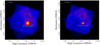 |
Fig. 1. NuSTAR FPMA+FPMB exposure-corrected images combined for the two observations of the field around 1E 1547.0–5408 over the 3–10 keV (left-hand panel) and 10–79 keV (right-hand panel) energy bands. North is up, East to the left. The roll angles were 208.3° and 162.8° for the first and the second observation, respectively, measured from North towards East. Both images were smoothed with a Gaussian filter with a kernel radius of 3 pixels (one NuSTAR FPM pixel corresponds to about 2.46 arcsec), and the same color code was applied to both cases. The green circle indicates the extraction region adopted to collect the source counts, while the dashed white circle marks an example of an extraction region used to estimate the background level (see the text for details). |
We applied the NUPRODUCTS tool to extract background-subtracted spectra and to generate instrumental response and auxiliary files for each FPM and for both observations. All photons outside the 3–79 keV energy interval were flagged as bad. Given the similarity of the net count rates along the two epochs (see above), we decided to combine all the spectra and response files to increase the photon counting statistics and better constrain the source spectral shape. The resulting background-subtracted spectrum was then grouped so as to contain at least 20 photons per energy bin. For the timing analysis, we referred the photon arrival times of the source event files to the Solar System barycenter using the BARYCORR tool and version 91 of the NuSTAR clock file to correct for drifts of the spacecraft clock3.
3. Analysis and results
3.1. Spectral analysis and long-term light curves
We modeled the Swift XRT spectra acquired since the beginning of 2012 within the XSPEC package (v. 12.10.1; Arnaud 1996) following the prescriptions reported by Coti Zelati et al. (2018): we employed an absorbed blackbody (BB) plus power law (PL) model, adopting the TBABS model with cross-sections of Verner et al. (1996) and elemental abundances of Wilms et al. (2000) to describe the photo-electric absorption by the interstellar medium along the line of sight. We fixed the column density to NH = 4.9 × 1022 cm−2 (see Coti Zelati et al. 2018).
As a first step, we allowed all the parameters to vary among the spectra. The best-fitting values for the BB temperature and radius and the PL photon index were found to be compatible with each other over the past ∼9 yr within a 2σ confidence level. To better constrain the temporal evolution of these parameters, we jointly fit the spectra acquired during the same year, tying up the above-mentioned parameters among the data sets. We obtained statistically acceptable results in all cases (the reduced chi-squared  ranged from 0.89 to 1.05). The BB temperature and emitting radius were between kTBB ∼ 0.6–0.8 keV and RBB ∼ 0.6–1.3 km, while the PL photon index varied between Γ ∼ 2.4–3.3. However, we did not observe any clear trend in the time evolution of these parameters.
The upper panel of Fig. 2 shows the combined spectra extracted from the NuSTAR and Swift XRT data acquired in WT-mode close to the epoch of the first NuSTAR observation (obs ID: 00030956189; exposure time of ∼1.7 ks). A change in the spectral slope can be clearly seen at an energy of ≈15 keV, calling for an additional spectral component at higher energies. Hence, we fitted different multi-component models to the NuSTAR plus Swift spectrum: a double-BB plus a PL model (2BB+PL), a BB plus a broken PL model (BB+2PL), and the resonant Compton scattering model NTZ (see Nobili et al. 2008) plus a PL component (NTZ+PL). The hydrogen column density was fixed to the values we obtained for the outbursts in 2008 and 2009 under the same assumptions for the absorption model (Coti Zelati et al. 2018), that is, NH = 4.9 × 1022 cm−2 for the BB+2PL model and NH = 4.6 × 1022 cm−2 for the 2BB and NTZ+PL models. A renormalization constant was also included to account for intercalibration uncertainties, and was found to be consistent within the 1σ uncertainties across the different instruments in all cases.
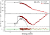 |
Fig. 2. Spectrum of 1E 1547.0–5408 extracted over the 0.7–70 keV energy band from the Swift XRT (black triangles) and merged NuSTAR data sets (red circles). Data points were re-binned for plotting purpose. The solid line represents the best-fitting BB+2PL model. The E2f(E) unfolded spectrum is shown in the middle panel. Dashed lines mark the contribution of the single components to the spectral model. Post-fit residuals in units of standard deviations are shown in the bottom panel. |
All three models provided satisfactory results ( , 0.97 and 0.99 for 301 d.o.f., for the 2BB+PL, BB+2PL and NTZ+PL models, respectively). The best-fitting values for the spectral parameters, the fluxes and the luminosities are listed in Table 1. Figure 2 shows the broad-band spectrum fitted with the BB+2PL model, the unfolded spectrum highlighting the contribution of the different components, and the post-fit residuals. We derived fully compatible results when modeling the NuSTAR spectrum together with the Swift XRT spectra acquired in PC mode in observations nearly simultaneous to the second NuSTAR observation (IDs: 00088680002, 00088680003 for a total exposure time of 3.3 ks). The observed fluxes in the 1–10 keV and 15–60 keV energy bands are
  erg cm−2 s−1 and
  erg cm−2 s−1, respectively (here and in the following, all uncertainties are quoted at a confidence level (c.l.) of 1σ). The flux hardness ratio, η = F15−60/F1−10 ≈ 0.6, is smaller than that obtained during past Suzaku observations in 2009 and 2010, η = 1.2−1.8 (see Enoto et al. 2017). However, it still follows the correlation between the spectral hardness and the dipole magnetic field reported by Enoto et al. (2017). To derive a constraint on the steepening of the hard PL component at high energies, we restricted our spectral analysis to energies above 13 keV, and fitted a PL model with high-energy exponential cutoff (CUTOFFPL in XSPEC) to the data. We inferred a lower limit on the high-energy roll-over of Ecut > 260 keV (3σ c.l.).
Results of the joint fits of the Swift spectrum and the combined spectrum extracted from the two NuSTAR observations of 1E 1547.0–5408.
Figure 3 shows the long-term evolution of the observed flux and of the luminosities for the single spectral components as well as the total one in the soft X-ray band. 1E 1547.0–5408 did not return to the level observed in 2006 following the three outbursts in 2007, 2008 and 2009. In particular, the X-ray flux over the past ∼9 yr has settled on a value of ≈10−11 erg cm−2 s−1. This is about an order of magnitude below the value at the peak of the 2009 outburst, a factor of ∼5 larger than those measured in 1980 and 1998, and a factor of ∼30 above that detected in July 2006.
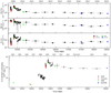 |
Fig. 3. Top: long-term evolution of the observed flux and of the luminosities of the BB and soft PL spectral components of 1E 1547.0–5408 between 2008 October 3 and 2019 February 15. Bottom: long-term evolution of the soft X-ray luminosity of 1E 1547.0–5408 between 2004 February 8 and 2019 February 15. The values derived from Chandra and XMM–Newton observations are taken from Coti Zelati et al. (2018). All quantities are evaluated over the 0.3–10 keV energy band. Luminosities have been estimated following the same procedure outlined in Table 1. The luminosities in the time interval between 2013 and 2017 are consistent with those measured after 2017, and are not shown for plotting purpose. |
The left-hand panel of Fig. 4 shows the time evolution of the flux (top) and spectral shape for the PL component (bottom) in the hard X-ray band since the onset of the 2009 outburst (when it was first detected), extracted using the values published by Enoto et al. (2010), Kuiper et al. (2012) and Iwahashi et al. (2013) for the archival observations. The hard X-ray flux measured in the recent NuSTAR observations, ∼7 × 10⁻¹² erg cm−2 s−1 over the 10–70 keV energy band, is a factor of ≈20 smaller than that measured at the peak over the same band. The PL gradually hardened in time, with the photon index decreasing from Γhard ∼ 1.4 about 3 days after the 2009 outburst onset (Kuiper et al. 2012), to Γhard ∼ 0 about ten years later (see also Table 1). We estimated the rate of the PL hardening by fitting an exponential function of the form  to the time evolution of the photon index (t represents the time since the outburst onset and τh the e-folding time). We obtained a good description of the data (
 for 6 d.o.f.; see the dashed light grey line in Fig. 4), and derived best-fitting parameters Γ0 = 1.45 ± 0.03 and
  d. All in all, the decrease of the hard X-ray flux in time appears to be accompanied by a hardening of the spectrum at high energies (see the right-hand panel of Fig. 4).
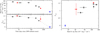 |
Fig. 4. Left: time evolution of the flux in the 10–70 keV energy band (top) and of the PL photon index in the hard X-rays (bottom) of 1E 1547.0–5408 since the onset of the last outburst on 2009 January 22 at 00:53 UTC. Black squares refer to INTEGRAL data, red triangles refer to Suzaku data, the blue star refers to the merged NuSTAR observations presented in this study. All fluxes for archival observations were referred to the 10–70 keV band using PIMMS (https://heasarc.gsfc.nasa.gov/cgi-bin/Tools/w3pimms/w3pimms.pl), assuming the spectral shapes reported in Table 3 by Enoto et al. (2010), Table 8 by Kuiper et al. (2012) and Table 3 by Iwahashi et al. (2013). The dashed grey line in the bottom panel denotes the best-fitting exponential function for the time evolution of the photon index (see the text for details). Right: evolution of the PL photon index for the hard X-ray component as a function of the hard X-ray flux. Marks and colors are the same as in the left panel. |
3.2. Pulse profiles and phase-resolved spectral analysis for the NuSTAR observations
We computed the  test (Buccheri et al. 1983) on the source event lists from the combined FPMA and FPMB data sets separately for the two observations. We detected a prominent peak at a period of P ∼ 2.08671 s in the first observation and P ∼ 2.08843 s in the second observation. We honed these values by dividing the time series of both observations in 6 time segments of approximately equal length, and applying a phase-fitting technique. Fitting a first order polynomial function to the phase evolution yielded P = 2.0867100(1) s at
  MJD and P = 2.0884305(3) s at
  MJD. This implies a net spin-down rate of ∼1.9 × 10⁻¹¹ s s−1 between April 2016 and February 2019.
The top and middle panels of Fig. 5 show the background-subtracted light curves extracted from the combined FPMA and FPMB data sets, folded on our best value for P measured in each observation. We detected pulsed emission up to ≈25 keV. The profile shape above 10 keV is apparently different from that observed at lower energies. Moreover, the peak of the pulse profile at higher energies appears to lag the peak at lower energies.
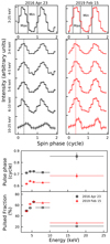 |
Fig. 5. Top: background-subtracted pulse profiles of 1E 1547.0–5408 extracted over the 3–25 keV energy range from the combined NuSTAR FPMA and FPMB data sets, and separately for both observations. The vertical black solid lines mark the phase intervals adopted to extract the phase-resolved spectra. Middle: pulse profiles extracted in selected energy ranges. The profiles have been shifted along the vertical axis for plotting purpose. The vertical dashed lines mark the phase of the pulse peak in the soft X-ray energy bands (up to 10 keV). All pulse profiles in the top and middle panels are sampled in 10 phase bins, and two phase cycles are shown. For display purposes, the 2016 pulse profiles have been phase-aligned to the 2019 ones. Bottom: pulse phase (top) and pulsed fraction (bottom) as a function of energy at both epochs. |
To evaluate the shift as well as the pulsed fraction values as a function of photon energy, we modeled the pulse profiles with a constant plus two sinusoidal functions, fixing the sinusoidal periods to those of the fundamental and second harmonic components. The inclusion of higher harmonic components in the fit was not statistically needed (F–test probability of 0.48 for the improvement in the fit). We evaluated the phase lags as the difference in the pulse phase of the fundamental component between the pulse profiles extracted over the 10–25 keV and 3–4 keV energy intervals (see the bottom panel of Fig. 5). We determined a phase lag of Δϕ1 = 0.15 ± 0.03 cycles in April 2016 and Δϕ2 = 0.07 ± 0.02 cycles in February 2019. We obtained compatible values when considering the 4–5 keV, 5–6 keV and 6–10 keV energy intervals as a reference for the soft X-ray band. We computed the pulsed fraction in the different energy intervals by dividing the value of the semi-amplitude for the fundamental component of the pulse profile by the average count rate. In both observations, the pulsed fraction shows an increasing trend up to 6 keV, from ∼49% in the 3–4 keV interval up to ∼65% in the 5–6 keV range. Then, it decreases at higher energies, down to ∼20–25% over the 10–25 keV energy range (see the bottom panel of Fig. 5). Pulsations are no more significantly detected at higher energies. We estimate 4σ upper limits on the pulsed fraction of 23% and 14% for the first and the second observation, respectively, over the 25–70 keV energy range.
The pulsed fraction at low energies is larger than that measured over the 1–6 keV energy range in 2006 (≈15%; Halpern et al. 2008). We reanalyzed the data taken in a 12-ks observation with Chandra ACIS-S (ID: 10186) on 2009 February 2, ∼10 d after the outburst onset. We detected the spin signal at P = 2.07211(1) s, and found pulsed fractions of ∼11% in the 3–4 and 4–5 keV ranges, ∼5 % in the 5–6 keV interval and ∼8% in the 6–10 keV range. Hence, the pulsed fraction increased considerably along the outburst decay in the soft X-ray energy bands. On the other hand, the detection of pulsed emission in the hard X-ray band appears quite surprising considering the decreasing trend of the pulsed fraction along the first year of the outburst, down to undetectable levels about 11 months after the outburst onset (Kuiper et al. 2012; see e.g. their Fig. 9), when the flux was a factor of ∼4.5 larger than the value measured in the recent NuSTAR observations (see the top panel of Fig. 4).
We performed a pulse phase-resolved spectral analysis for both NuSTAR observations using data from both FPMs. For each observation, we extracted the spectra within the phase intervals corresponding to the maximum and the minimum of the pulse profiles (these intervals were selected as indicated in the top panel of Fig. 5). We then combined the spectra for the maximum and the minimum from the two observations to increase the photon counting statistics4, and fitted them together using an absorbed BB+2PL model (the column density was fixed at the phase-averaged value). The BB temperatures were found to be consistent with each other and with the phase-averaged value, and were thus fixed to that value in the spectral fits. We obtained an acceptable result, with  (284 d.o.f.). The spectral shape changes significantly as a function of the rotational phase (see Fig. 6). We derived the following parameters: Γsoft, max = 3.4 ± 0.1, Γhard, max = 0.5 ± 0.3, Ebreak, max = (13.1 ± 0.6) keV at the maximum; Γsoft, min = 4.20 ± 0.09, Γhard, min = 1.0 ± 0.1, Ebreak, min = (9.2 ± 0.2) keV at the minimum.
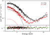 |
Fig. 6. Top: E2f(E) unfolded spectra of 1E 1547.0–5408 extracted from the merged NuSTAR data sets at the maximum (in black) and at the minimum (in red) of the pulse profile. Data points were re-binned for plotting purpose. The solid lines represent the best-fitting BB+2PL model. Dashed lines mark the contribution of the single components to the spectral model. Bottom: post-fit residuals in units of standard deviations. |
4. Discussion
4.1. A very slow luminosity decay?
The long-term light curve of 1E 1547.0–5408 in the soft X-ray band since the onset of its last outburst in 2009 reveals an initial decay by one order of magnitude in flux over the first year (see Fig. 3). Such a decay pattern is typically observed for magnetar outbursts (Coti Zelati et al. 2018). However, in the past 9 years, the source has always maintained a flux of ≈10−11 erg cm−2 s−1 which is a factor of ∼30 above the value measured in 2006, and a factor of ∼5 larger than the values observed in 1980 and 1998. Such a prolonged, possibly persistent, high X-ray flux is a property that, so far, has not been seen so clearly in other magnetars. The long-lasting high temperature (kTBB ≳ 0.6 keV) is an additional feature that so far has been observed over a few years only in other few cases, e.g. during the recent outbursts of the magnetars SGR J1745−2900 (Coti Zelati et al. 2015, 2017) and CXOU J1647–4552 (Borghese et al. 2019).
On the other hand, the conspicuous softening of the PL component in the soft X-rays (from Γ ∼ 1.2 at the outburst peak to Γ ∼ 3.8 about a decade later), the reduction of the BB emitting radius (from RBB ∼ 3 km down to RBB ∼ 1 km) and the weakening of the hard X-ray tail are all properties commonly seen in magnetars along the outburst decay (e.g., Kaspi & Beloborodov 2017; Esposito et al. 2018). The current broad-band X-ray properties of 1E 1547.0–5408 are also very similar to those observed in other magnetars. Changes in the profile structure with energy are observed in 1RXS J170849−400910 (Götz et al. 2007; den Hartog et al. 2008), 1E 1841−045 (An et al. 2015), 1E 2259+586 (Vogel et al. 2014), 4U 0142+61 (Tendulkar et al. 2015), 1E 1048.1−5937 (Yang et al. 2016), XTE J1810−197 (Gotthelf et al. 2019), SGR 1900+14 (Tamba et al. 2019). The pulse profiles of 1RXS J170849−400910, 1E 2259+586 and XTE J1810−197 also display a phase shift with energy. All these magnetars also show some degree of variability of the pulsed fraction with energy, as well as of the hard X-ray spectral shape along the rotational phase cycle.
In the following, we focus on the unusual long-term evolution of the X-ray flux of 1E 1547.0–5408 over the last decade. In a recent systematic study of magnetar outbursts (Coti Zelati et al. 2018), we characterized the post-outburst luminosity trend of a large sample of magnetars using a simple phenomenological model. In that work, the luminosity decay was fit using an exponential function with two free parameters:
 (1)
(1)
where Lmax is the luminosity at the outburst peak, L0 is the value to which the luminosity tends to decay, t is the time elapsed since the epoch of the outburst peak, and τ is the e-folding time. It was assumed that L0 corresponds to the pre-outburst luminosity (i.e., that each source returns back to the pre-outburst level, and that L0 is always the same for a given source).
The simple model above was used to predict the decay timescale, that is how long the luminosity takes to return to a value compatible with that before the outburst (the luminosity measured in 2006 for the case of 1E 1547.0–5408), as well as the total extra energy released during the outburst Eout = τ(Lmax − L0).
In a few cases, the functional form provided by Eq. (1) was too simple and a second exponential function was needed to fit adequately the data:
![Mathematical equation: $$ \begin{aligned} L(t)= (L_{\mathrm{max}} - L_0)\,[e^{-t/\tau _1}+e^{-t/\tau _2}] + L_0. \end{aligned} $$](/articles/aa/full_html/2020/01/aa36317-19/aa36317-19-eq20.gif) (2)
(2)
This is also the case for the 2009 outburst of 1E 1547.0–5408, if we apply the same procedure: once L0 is fixed to 2.2 × 1033 erg s−1 (i.e., the value measured in 2006; see Fig. 3), the best-fitting decay model is represented by a double-exponential function with τ1 = 164 ± 43 d and  d (yielding
  for 287 d.o.f.).
Figure 7 shows the energy emitted from magnetars during powerful outbursts as a function of the outburst decay timescale. Based on the extrapolation of the model above (i.e., assuming no changes in the decay pattern), we estimated that 1E 1547.0–5408 would return to a luminosity similar to that measured in 2006 (within ≲10%) in ≈50 yr, releasing an energy of Eout ∼ 7.3 × 1043 erg. These characteristics would make the 2009 event from 1E 1547.0–5408 by far the longest magnetar outburst ever observed (see the blue square in Fig. 7). For a comparison, the second longest outburst hitherto detected according to our models is the 1998 episode from SGR 1627–41, for which the long-term light curve can be described by a double-exponential function with τ1 ∼ 234 d and τ2 ∼ 1310 d. The value of the outburst energy for 1E 1547.0–5408 would be also exceptionally large, even larger than that estimated for SGR 1806−20 after the giant flare in December 2004, that is ∼2 × 1043 erg5.
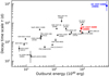 |
Fig. 7. Decay timescale (in terms of the e-folding time τ) as a function of the total energy released for all magnetar outbursts detected so far. For the cases where more exponential functions were adopted to model the light curve, the value of τ corresponding to the exponential function modeling the late-time evolution of the outburst was considered. The blue square refers to the case where 1E 1547.0–5408 is assumed to return to the 2006 level. The red star refers instead to the case where 1E 1547.0–5408 is assumed to have settled on a new persistent state over the last years. In a few cases, the size of the marker is larger than the error bars. Adapted from Borghese et al. (2019). |
The results obtained with the simple model above rely on the assumption that the value for L0 is equal to that observed before the outburst, meaning that magnetars are characterized by a quiescent state which remains the same over decades. However, there is virtually no observation for any magnetar which guarantees that their persistent luminosity remains actually constant over these timescales. If we relax the assumption of a fixed L0 in the light curve modeling of 1E 1547.0–5408, we obtain  for 286 d.o.f. The F-test yields a null hypothesis probability for the improvement of the fit of ≃6 × 10⁻⁶, implying that a model where L0 is allowed to vary provides a more accurate description of the luminosity evolution. The best-fitting parameters are
  d,
d,  d, L0 = (6 ± 1)×1034 erg s−1 and Eout ∼ 9 × 1042 erg. Hence, in this case, both the decay timescale and the energetics greatly reduce compared to the fit outlined above. These would be more in line with the values estimated for other magnetar outbursts (see the red star in Fig. 7).
The assumption of a fixed L0 is tightly connected to the physical mechanisms that trigger and sustain the outburst activity of magnetars, as described in the following sections.
4.2. Crustal cooling or coronal activity?
The emission observed during magnetar outbursts has been commonly interpreted as the result of the progressive cooling of a thermally-emitting hot spot on the star surface. The hot spot can be formed, arguably, owing to two different, but not mutually excluding, mechanisms. The first one is the sudden release of heat in the crust due to the long-term building-up of magnetic stresses in the crust, causing either a starquake (e.g. Perna & Pons 2011; Pons & Perna 2011; Pons & Rea 2012; Thompson et al. 2017) or a thermoplastic wave (Beloborodov & Levin 2014; Li et al. 2016). The second mechanism is the Ohmic dissipation and or particle bombardment upon the star surface due to the currents circulating in the magnetar corona (e.g. Beloborodov 2009, 2013a,b; Beloborodov & Li 2016; Chen & Beloborodov 2017).
On the one hand, in the crustal cooling scenario, the persistent luminosity L0 is expected to arise from the internal heat diffusion, which yields changes over timescales ≳103–104 yr (assuming a kyr-aged magnetar; see e.g. Viganò et al. 2013; Potekhin et al. 2015) that are longer than any observable time span. Hence, this scenario predicts that each source should approximately recover the pre-outburst temperature and thermal luminosity. According to this scenario, the size of the emitting region should increase in time due to heat spreading across the crustal layers and the envelope. In general, crustal cooling from a single heat release cannot sustain long-lived (several years) surface temperatures of kT ≳ 0.5 keV. Hence, to explain the behaviour of 1E 1547.0–5408 in terms of crustal cooling alone, a repeated or continuous heating would be required. Such a heating should be shallow, otherwise an enormous input energy would be required. However, crustal cooling alone cannot account for non-thermal hard X-ray emission, such as that observed in 1E 1547.0–5408.
On the other hand, in the coronal currents scenario, the currents are responsible for both thermal X-ray emission, via their slow dissipation in localized regions close to the surface of the star, which is highly resistive (e.g. González-Caniulef et al. 2019), and non-thermal X-ray emission, via resonant inverse Compton scattering of photons from the surface by the charged particles (e.g. Turolla et al. 2015). The resonant Compton scattering can manifest in the form of distinct soft and hard X-ray emission components. The former is fed by mildly relativistic charges, the latter by ultra-relativistic charges moving along an extended (≲10 stellar radii) closed twisted magnetic loop around the star. The up-scattered photons convert to electron-positron pairs close to the star surface. The radiated energy is processed into a relativistic outflow of pairs that experiences a radiative drag as it propagates away from the star, and annihilates at the top of the loop. A dominant contribution from long-lived coronal currents to the emitted radiation can account naturally for the shrinking of the emitting region and the relatively high temperatures observed in 1E 1547.0–5408 along the outburst decay (and seen also in several other magnetars; see e.g. Alford & Halpern 2016; Coti Zelati et al. 2017; Borghese et al. 2018). It can also explain adequately a number of broad-band spectral and timing properties observed for this source over the past few years:
-
(i)
the emergent spectra of the resonant Compton scattering for mono-energetic uncooled relativistic electrons moving along field loops have been computed by Wadiasingh et al. (2018). The slope of the PL tail at high energies is determined by the electron Lorentz factor, the loop orientation and the scattering kinematics. It strongly depends on the viewing angle and the location of resonant scattering, and is thus predicted to vary as a function of the rotational phase. This predicted behavior is consistent with our detection of a marked change in the values for the spectral parameters at the maximum and the minimum of the pulse profile in 1E 1547.0–5408;
-
(ii)
the hard X-ray emission is expected to be beamed along the magnetic loop, leading to detectable pulsed emission. The pulse profile shape strongly depends on the complex geometry of the emission from the electron-positron outflow, as well as the relative contribution of possible multiple loops to the observed emission (Wadiasingh et al. 2018). The loop does not necessarily extend above the small thermally-emitting hot spot on the star surface, along the line of sight. This is consistent with our detection of a misalignment between the peaks in the soft and hard X-ray pulse profiles of 1E 1547.0–5408. Photons are presumably up-scattered at different locations along the extended loop (i.e., at different heights above the stellar surface). Consequently, the hard X-ray emission shall be less anisotropic than the soft X-ray emission from the hot spot on the star surface. This is consistent with the smaller values for the pulsed fraction at higher energies in 1E 1547.0–5408.
Hence, while both crustal cooling and coronal activity might be possibly at work in other magnetars, the properties observed for 1E 1547.0–5408 seem to favour the latter scenario. However, besides this interpretative dichotomy (which is applicable to several other magnetars), the flux evolution of 1E 1547.0–5408 gives some additional new clues, as discussed in the next section.
4.3. A new persistent coronal state?
Our analysis suggests that 1E 1547.0–5408 is actually not decaying in luminosity any longer and has reached a persistent magnetospheric state that is different from the state observed in 2006, when the source was found at a much smaller luminosity. Such an interpretation is corroborated by the remarkable difference between the values for the pulsed fraction measured at low energies in the past few years and in 2006.
A magnetospheric reconnection, most likely triggered by a sudden event in the crust (a thermoplastic wave or a starquake) can lead to a local reorganization of the magnetic field, leaving in the wake of the transient event a new pattern of twisted field associated to current bundles that close within the envelope and the crust. Carrasco et al. (2019) performed 3D relativistic force-free simulations of the magnetospheric outburst due to the progressive twisting of the line footprints at the surface, extending previous axisymmetric non-relativistic simulations (Parfrey et al. 2013). When a critical twist is reached, the magnetosphere undergoes a state of instability. This, in turn, leads to a rapid expansion of the lines, which finally reconnect, expelling plasmoids. After this rapid (millisecond-long) phase, a new state is reached, with non-negligible currents threading the magnetosphere.
The key issue is then to assess the survival timescale of the magnetospheric currents. A phenomenological estimate can be obtained simply by assuming that the measured luminosity ultimately comes from Ohmic dissipation of the magnetic twist: tstate ∼ Etwist/LX, where Etwist is the free magnetic energy contained in the twisted bundle. According to 3D (Carrasco et al. 2019) and 2D (Beloborodov 2009; Parfrey et al. 2013) simulations, this magnetic energy is typically a fraction ffree ∼ 0.01–0.1 of the total energy budget, so that  , with B14 = Bp/1014 G and R10 = R⋆/10 km. Thus we get
 (3)
(3)
where L35 is the thermal luminosity in units of 1035 erg s−1. For a large enough free magnetic energy,  (i.e., a large twist and or a large background field), bundles could dissipate in tens of years, thus providing a persistent emission that is apparently constant on the typical observation timescales. On the other hand, smaller twists (associated to a smaller free magnetic energy) should dissipate faster. The estimate provided by Eq. (3) represents an upper limit, since it implicitly assumes a perfect efficiency in the Ohmic to radiative blackbody surface radiation. The more the Ohmic dissipation along the circuit is localized close to the surface, the more the approximation is correct.
A different, first-principles assessment of the survival timescales is provided by Beloborodov (2009). Using the estimate by Beloborodov & Thompson (2007) for the electrical potential along a field line due to pair production and electrical discharge, he infers values in the range from years to decades (depending on the uncertain input parameters). These estimates were obtained from an axially symmetric calculation, assuming that the magnetosphere is globally twisted and that the star, where the current loops close, is perfectly conductive. However, the latter assumption is not accurate when considering the external envelope. As a matter of fact, preliminary estimates have shown that the very high resistivity of the outermost layers (with depths of meters or tens of meters) can account for the prolonged high temperatures observed for magnetars, if one supposes that most of the Ohmic dissipation of the magnetospheric currents occurs there (Akgün et al. 2018; Carrasco et al. 2019). These approximate estimates should then be fine-tuned by a better understanding and a more detailed computation of the total impedence along the current loops (dominated by the contribution from the magnetosphere and the envelope). Given their lack and the considerable uncertainties, the predicted timescales for the dissipation are compatible with the typical time span over which magnetars have been observed to linger at roughly the same flux (about a decade or so).
5. Conclusions
We studied the long-term evolution of the X-ray emission properties of the magnetar 1E 1547.0–5408 since February 2004, reanalyzing its three outbursts using new and archival observations with Swift, NuSTAR, Chandra, and XMM–Newton. About one year after the last outburst in 2009, the source settled on a relatively steady high flux level, a factor of ∼30 larger than its quiescent flux in 2006. Recent NuSTAR observations revealed faint hard X-ray emission up to about 70 keV, and showed a peculiar progressive flattening of the high-energy power law spectral component in time. This is at variance with the cooling trend observed for the soft X-ray component, as well as with the typical overall gradual softening observed in other magnetar outbursts (see e.g. Esposito et al. 2018).
1E 1547.0–5408 provides compelling evidence that the persistent X-ray luminosity of magnetars should be necessarily dominated by magnetospheric currents, which are responsible for both surface heating (in the form of thermal emission) and resonant Compton scattering (non-thermal soft and hard X-ray emissions). In fact, peculiar signatures for such a dominant magnetospheric component would be: (i) frequent changes between different persistent luminosities (not viable with internal crustal cooling alone); (ii) comparatively large persistent temperatures; (iii) small – and possibly shrinking – size of the emitting regions.
Currently, not all magnetar outbursts have been followed over a long enough timescale to claim the full recovery to the pre-outburst level (Coti Zelati et al. 2018). However, except for 1E 1547.0–5408, none of the sources monitored so far have shown such a large difference between their post-outburst steady flux and their previous quiescent level.
In the near future, an on-going monitoring campaign with NICER (PI: A. Borghese; Borghese et al., in prep.) might reveal any peculiar timing behaviour possibly connected with the new state reached by 1E 1547.0–5408. Radio observations will also be valuable to reveal possible magnetospheric changes. Future Swift observations will play a crucial role to probe the flux steadiness of 1E 1547.0–5408 over an even more extended time span and further characterize the emission properties of a magnetar that, at present, has no equal within this class of sources.
Very similar parameter values were derived from the spectral analysis of the datasets separately at the two different epochs.
The value estimated for SGR 1806−20 represents, however, only a lower limit, because the source flux was already increasing by a factor of ∼2 during the first half of 2004 with respect to the level observed previously (Mereghetti et al. 2005).
Acknowledgments
We thank the referee for helpful and valuable comments. FCZ acknowledges Matthew Baring for helpful discussions. FCZ, AB, NR and DV acknowledge support from grants SGR2017-1383 and PGC2018-095512-B-I00 and the support of the PHAROS COST Action (CA16214). FCZ is also supported by a Juan de la Cierva fellowship. NR, AB and DV are also supported by the ERC Consolidator Grant “MAGNESIA” (nr. 817661). DV acknowledges support from grants AYA2016-80289-P and AYA2017-82089-ERC. TE is supported by JSPS KAKENHI grant numbers 16H02198, 18H01246 and 18H04584. JAP acknowledges support from the Spanish Agencia Estatal de Investigación (grant PGC2018-095984-B-I00) and the Generalitat Valenciana (grant PROMETEO/2019/071). The scientific results reported in this article are based on data obtained with Swift, the Chandra X-ray Observatory, XMM–Newton and the NuSTAR mission. XMM–Newton is an ESA science mission with instruments and contributions directly funded by ESA Member States and the National Aeronautics and Space Administration (NASA). The NuSTAR mission is a project led by the California Insitute of Technology, managed by the Jet Propulsion Laboratory, and funded by NASA. We made use of data supplied by the UK Swift Science Data Centre at the University of Leicester and of the XRT Data Analysis Software (XRTDAS) developed under the responsibility of the ASI Science Data Center (ASDC), Italy. We also made use of the NuSTAR Data Analysis Software (NUSTARDAS jointly developed by the ASI Science Data Center (ASDC, Italy) and the California Institute of Technology (USA), and of softwares and tools provided by the High Energy Astrophysics Science Archive Research Center (HEASARC), which is a service of the Astrophysics Science Division at NASA/GSFC and the High Energy Astrophysics Division of the Smithsonian Astrophysical Observatory.
References
- Akgün, T., Cerdá-Durán, P., Miralles, J. A., & Pons, J. A. 2018, MNRAS, 481, 5331 [NASA ADS] [CrossRef] [Google Scholar]
- Alford, J. A. J., & Halpern, J. P. 2016, ApJ, 818, 122 [NASA ADS] [CrossRef] [Google Scholar]
- An, H., Archibald, R. F., Hascoët, R., et al. 2015, ApJ, 807, 93 [NASA ADS] [CrossRef] [Google Scholar]
- Arnaud, K. A. 1996, in Astronomical Data Analysis Software and Systems V, eds. G. H. Jacoby, & J. Barnes, ASP Conf. Ser., 101, 17 [NASA ADS] [Google Scholar]
- Beloborodov, A. M. 2009, ApJ, 703, 1044 [NASA ADS] [CrossRef] [Google Scholar]
- Beloborodov, A. M. 2013a, ApJ, 777, 114 [NASA ADS] [CrossRef] [Google Scholar]
- Beloborodov, A. M. 2013b, ApJ, 762, 13 [NASA ADS] [CrossRef] [Google Scholar]
- Beloborodov, A. M., & Levin, Y. 2014, ApJ, 794, L24 [NASA ADS] [CrossRef] [Google Scholar]
- Beloborodov, A. M., & Li, X. 2016, ApJ, 833, 261 [NASA ADS] [CrossRef] [Google Scholar]
- Beloborodov, A. M., & Thompson, C. 2007, ApJ, 657, 967 [NASA ADS] [CrossRef] [Google Scholar]
- Bernardini, F., Israel, G. L., Stella, L., et al. 2011, A&A, 529, A19 [NASA ADS] [CrossRef] [EDP Sciences] [Google Scholar]
- Borghese, A., Coti Zelati, F., Esposito, P., et al. 2018, MNRAS, 478, 741 [NASA ADS] [CrossRef] [Google Scholar]
- Borghese, A., Rea, N., Turolla, R., et al. 2019, MNRAS, 484, 2931 [NASA ADS] [CrossRef] [Google Scholar]
- Buccheri, R., Bennett, K., Bignami, G. F., et al. 1983, A&A, 128, 245 [NASA ADS] [Google Scholar]
- Burrows, D. N., Hill, J. E., Nousek, J. A., et al. 2005, Space Sci. Rev., 120, 165 [NASA ADS] [CrossRef] [Google Scholar]
- Camilo, F., Ransom, S. M., Halpern, J. P., & Reynolds, J. 2007, ApJ, 666, L93 [NASA ADS] [CrossRef] [Google Scholar]
- Carrasco, F., Viganò, D., Palenzuela, C., & Pons, J. A. 2019, MNRAS, 484, L124 [NASA ADS] [CrossRef] [Google Scholar]
- Chen, A. Y., & Beloborodov, A. M. 2017, ApJ, 844, 133 [NASA ADS] [CrossRef] [Google Scholar]
- Coti Zelati, F., Rea, N., Papitto, A., et al. 2015, MNRAS, 449, 2685 [NASA ADS] [CrossRef] [Google Scholar]
- Coti Zelati, F., Rea, N., Turolla, R., et al. 2017, MNRAS, 471, 1819 [NASA ADS] [CrossRef] [Google Scholar]
- Coti Zelati, F., Rea, N., Pons, J. A., Campana, S., & Esposito, P. 2018, MNRAS, 474, 961 [NASA ADS] [CrossRef] [Google Scholar]
- den Hartog, P. R., Kuiper, L., & Hermsen, W. 2008, A&A, 489, 263 [NASA ADS] [CrossRef] [EDP Sciences] [Google Scholar]
- Dib, R., Kaspi, V. M., Scholz, P., & Gavriil, F. P. 2012, ApJ, 748, 3 [NASA ADS] [CrossRef] [Google Scholar]
- Enoto, T., Nakazawa, K., Makishima, K., et al. 2010, PASJ, 62, 475 [NASA ADS] [CrossRef] [Google Scholar]
- Enoto, T., Shibata, S., Kitaguchi, T., et al. 2017, ApJS, 231, 8 [NASA ADS] [CrossRef] [Google Scholar]
- Esposito, P., Rea, N., & Israel, G. L. 2018, ArXiv e-prints [arXiv:1803.05716] [Google Scholar]
- Gelfand, J. D., & Gaensler, B. M. 2007, ApJ, 667, 1111 [NASA ADS] [CrossRef] [Google Scholar]
- González-Caniulef, D., Zane, S., Turolla, R., & Wu, K. 2019, MNRAS, 483, 599 [NASA ADS] [CrossRef] [Google Scholar]
- Gotthelf, E. V., Halpern, J. P., Alford, J. A. J., et al. 2019, ApJ, 874, L25 [NASA ADS] [CrossRef] [Google Scholar]
- Götz, D., Rea, N., Israel, G. L., et al. 2007, A&A, 475, 317 [NASA ADS] [CrossRef] [EDP Sciences] [Google Scholar]
- Halpern, J. P., Gotthelf, E. V., Reynolds, J., Ransom, S. M., & Camilo, F. 2008, ApJ, 676, 1178 [NASA ADS] [CrossRef] [Google Scholar]
- Harrison, F. A., Craig, W. W., Christensen, F. E., et al. 2013, ApJ, 770, 103 [NASA ADS] [CrossRef] [Google Scholar]
- Israel, G. L., Esposito, P., Rea, N., et al. 2010, MNRAS, 408, 1387 [NASA ADS] [CrossRef] [Google Scholar]
- Iwahashi, T., Enoto, T., Yamada, S., et al. 2013, PASJ, 65, 52 [NASA ADS] [CrossRef] [Google Scholar]
- Kaspi, V. M., & Beloborodov, A. M. 2017, ARA&A, 55, 261 [NASA ADS] [CrossRef] [Google Scholar]
- Kuiper, L., Hermsen, W., den Hartog, P. R., & Urama, J. O. 2012, ApJ, 748, 133 [NASA ADS] [CrossRef] [Google Scholar]
- Lamb, R. C., & Markert, T. H. 1981, ApJ, 244, 94 [NASA ADS] [CrossRef] [Google Scholar]
- Li, X., Levin, Y., & Beloborodov, A. M. 2016, ApJ, 833, 189 [NASA ADS] [CrossRef] [Google Scholar]
- Mereghetti, S., Tiengo, A., Esposito, P., et al. 2005, ApJ, 628, 938 [NASA ADS] [CrossRef] [Google Scholar]
- Ng, C. Y., Kaspi, V. M., Dib, R., et al. 2011, ApJ, 729, 131 [NASA ADS] [CrossRef] [Google Scholar]
- Nobili, L., Turolla, R., & Zane, S. 2008, MNRAS, 386, 1527 [NASA ADS] [CrossRef] [Google Scholar]
- Parfrey, K., Beloborodov, A. M., & Hui, L. 2013, ApJ, 774, 92 [NASA ADS] [CrossRef] [Google Scholar]
- Perna, R., & Pons, J. A. 2011, ApJ, 727, L51 [NASA ADS] [CrossRef] [Google Scholar]
- Pintore, F., Mereghetti, S., Tiengo, A., et al. 2017, MNRAS, 467, 3467 [NASA ADS] [CrossRef] [Google Scholar]
- Pons, J. A., & Perna, R. 2011, ApJ, 741, 123 [NASA ADS] [CrossRef] [Google Scholar]
- Pons, J. A., & Rea, N. 2012, ApJ, 750, L6 [NASA ADS] [CrossRef] [Google Scholar]
- Potekhin, A. Y., Pons, J. A., & Page, D. 2015, Space Sci. Rev., 191, 239 [NASA ADS] [CrossRef] [Google Scholar]
- Rea, N., Borghese, A., Esposito, P., et al. 2016, ApJ, 828, L13 [NASA ADS] [CrossRef] [Google Scholar]
- Savchenko, V., Neronov, A., Beckmann, V., Produit, N., & Walter, R. 2010, A&A, 510, A77 [NASA ADS] [CrossRef] [EDP Sciences] [Google Scholar]
- Scholz, P., & Kaspi, V. M. 2011, ApJ, 739, 94 [NASA ADS] [CrossRef] [Google Scholar]
- Tamba, T., Bamba, A., Odaka, H., & Enoto, T. 2019, PASJ, 71, 90 [NASA ADS] [CrossRef] [Google Scholar]
- Tendulkar, S. P., Hascöet, R., Yang, C., et al. 2015, ApJ, 808, 32 [NASA ADS] [CrossRef] [Google Scholar]
- Thompson, C., Yang, H., & Ortiz, N. 2017, ApJ, 841, 54 [NASA ADS] [CrossRef] [Google Scholar]
- Tiengo, A., Vianello, G., Esposito, P., et al. 2010, ApJ, 710, 227 [NASA ADS] [CrossRef] [Google Scholar]
- Turolla, R., Zane, S., & Watts, A. L. 2015, Rep. Prog. Phys., 78, 116901 [Google Scholar]
- Verner, D. A., Ferland, G. J., Korista, K. T., & Yakovlev, D. G. 1996, ApJ, 465, 487 [NASA ADS] [CrossRef] [Google Scholar]
- Viganò, D., Rea, N., Pons, J. A., et al. 2013, MNRAS, 434, 123 [NASA ADS] [CrossRef] [Google Scholar]
- Vogel, J. K., Hascoët, R., Kaspi, V. M., et al. 2014, ApJ, 789, 75 [NASA ADS] [CrossRef] [Google Scholar]
- Wadiasingh, Z., Baring, M. G., Gonthier, P. L., & Harding, A. K. 2018, ApJ, 854, 98 [NASA ADS] [CrossRef] [Google Scholar]
- Wilms, J., Allen, A., & McCray, R. 2000, ApJ, 542, 914 [NASA ADS] [CrossRef] [Google Scholar]
- Yang, C., Archibald, R. F., Vogel, J. K., et al. 2016, ApJ, 831, 80 [NASA ADS] [CrossRef] [Google Scholar]
All Tables
Results of the joint fits of the Swift spectrum and the combined spectrum extracted from the two NuSTAR observations of 1E 1547.0–5408.
All Figures
|
Fig. 1. NuSTAR FPMA+FPMB exposure-corrected images combined for the two observations of the field around 1E 1547.0–5408 over the 3–10 keV (left-hand panel) and 10–79 keV (right-hand panel) energy bands. North is up, East to the left. The roll angles were 208.3° and 162.8° for the first and the second observation, respectively, measured from North towards East. Both images were smoothed with a Gaussian filter with a kernel radius of 3 pixels (one NuSTAR FPM pixel corresponds to about 2.46 arcsec), and the same color code was applied to both cases. The green circle indicates the extraction region adopted to collect the source counts, while the dashed white circle marks an example of an extraction region used to estimate the background level (see the text for details). |
| In the text | |
|
Fig. 2. Spectrum of 1E 1547.0–5408 extracted over the 0.7–70 keV energy band from the Swift XRT (black triangles) and merged NuSTAR data sets (red circles). Data points were re-binned for plotting purpose. The solid line represents the best-fitting BB+2PL model. The E2f(E) unfolded spectrum is shown in the middle panel. Dashed lines mark the contribution of the single components to the spectral model. Post-fit residuals in units of standard deviations are shown in the bottom panel. |
| In the text | |
|
Fig. 3. Top: long-term evolution of the observed flux and of the luminosities of the BB and soft PL spectral components of 1E 1547.0–5408 between 2008 October 3 and 2019 February 15. Bottom: long-term evolution of the soft X-ray luminosity of 1E 1547.0–5408 between 2004 February 8 and 2019 February 15. The values derived from Chandra and XMM–Newton observations are taken from Coti Zelati et al. (2018). All quantities are evaluated over the 0.3–10 keV energy band. Luminosities have been estimated following the same procedure outlined in Table 1. The luminosities in the time interval between 2013 and 2017 are consistent with those measured after 2017, and are not shown for plotting purpose. |
| In the text | |
|
Fig. 4. Left: time evolution of the flux in the 10–70 keV energy band (top) and of the PL photon index in the hard X-rays (bottom) of 1E 1547.0–5408 since the onset of the last outburst on 2009 January 22 at 00:53 UTC. Black squares refer to INTEGRAL data, red triangles refer to Suzaku data, the blue star refers to the merged NuSTAR observations presented in this study. All fluxes for archival observations were referred to the 10–70 keV band using PIMMS (https://heasarc.gsfc.nasa.gov/cgi-bin/Tools/w3pimms/w3pimms.pl), assuming the spectral shapes reported in Table 3 by Enoto et al. (2010), Table 8 by Kuiper et al. (2012) and Table 3 by Iwahashi et al. (2013). The dashed grey line in the bottom panel denotes the best-fitting exponential function for the time evolution of the photon index (see the text for details). Right: evolution of the PL photon index for the hard X-ray component as a function of the hard X-ray flux. Marks and colors are the same as in the left panel. |
| In the text | |
|
Fig. 5. Top: background-subtracted pulse profiles of 1E 1547.0–5408 extracted over the 3–25 keV energy range from the combined NuSTAR FPMA and FPMB data sets, and separately for both observations. The vertical black solid lines mark the phase intervals adopted to extract the phase-resolved spectra. Middle: pulse profiles extracted in selected energy ranges. The profiles have been shifted along the vertical axis for plotting purpose. The vertical dashed lines mark the phase of the pulse peak in the soft X-ray energy bands (up to 10 keV). All pulse profiles in the top and middle panels are sampled in 10 phase bins, and two phase cycles are shown. For display purposes, the 2016 pulse profiles have been phase-aligned to the 2019 ones. Bottom: pulse phase (top) and pulsed fraction (bottom) as a function of energy at both epochs. |
| In the text | |
|
Fig. 6. Top: E2f(E) unfolded spectra of 1E 1547.0–5408 extracted from the merged NuSTAR data sets at the maximum (in black) and at the minimum (in red) of the pulse profile. Data points were re-binned for plotting purpose. The solid lines represent the best-fitting BB+2PL model. Dashed lines mark the contribution of the single components to the spectral model. Bottom: post-fit residuals in units of standard deviations. |
| In the text | |
|
Fig. 7. Decay timescale (in terms of the e-folding time τ) as a function of the total energy released for all magnetar outbursts detected so far. For the cases where more exponential functions were adopted to model the light curve, the value of τ corresponding to the exponential function modeling the late-time evolution of the outburst was considered. The blue square refers to the case where 1E 1547.0–5408 is assumed to return to the 2006 level. The red star refers instead to the case where 1E 1547.0–5408 is assumed to have settled on a new persistent state over the last years. In a few cases, the size of the marker is larger than the error bars. Adapted from Borghese et al. (2019). |
| In the text | |
Current usage metrics show cumulative count of Article Views (full-text article views including HTML views, PDF and ePub downloads, according to the available data) and Abstracts Views on Vision4Press platform.
Data correspond to usage on the plateform after 2015. The current usage metrics is available 48-96 hours after online publication and is updated daily on week days.
Initial download of the metrics may take a while.