| Issue |
A&A
Volume 633, January 2020
|
|
|---|---|---|
| Article Number | A27 | |
| Number of page(s) | 8 | |
| Section | Interstellar and circumstellar matter | |
| DOI | https://doi.org/10.1051/0004-6361/201935021 | |
| Published online | 03 January 2020 | |
Kinematic study of the molecular gas associated with two cometary globules in Sh2−236
1
CONICET – Universidad de Buenos Aires, Instituto de Astronomía y Física del Espacio (IAFE),
CP 1428 Buenos Aires,
Argentina
e-mail: This email address is being protected from spambots. You need JavaScript enabled to view it.
2
Universidad de Buenos Aires, Facultad de Arquitectura, Diseño y Urbanismo,
Buenos Aires,
Argentina
3
Departamento de Astronomía, Universidad de Chile,
Casilla 36-D,
Santiago,
Chile
Received:
4
January
2019
Accepted:
14
November
2019
Abstract
Aims. Cometary globules, dense molecular gas structures exposed to UV radiation, are found inside H II regions. Understanding the nature and origin of these structures through a kinematic study of the molecular gas could be useful to advance in our knowledge of the interplay between radiation and molecular gas.
Methods. Using the Atacama Submillimeter Telescope Experiment (Chile), we carried out molecular observations toward two cometary globules (Sim129 and Sim130) in the H II region Sh2−236. We mapped two regions of about 1′ × 1′ with the 12CO J = 3−2 and HCO+ J = 4−3 lines. Additionally, we carried out two single pointings with the C2H N = 4–3, HNC, and HCN J = 4−3 transitions. The angular resolution was about 22′′. We combined our molecular observations with public infrared and optical data to analyze the distribution and kinematics of the molecular gas.
Results. We find kinematic signatures of infalling gas in the 12CO J = 3−2 and C2H N = 4−3 spectra toward Sim 129. We detect HCO+, HCN, and HNC J = 4−3 only toward Sim 130. The HCN/HNC integrated ratio of about three found in Sim 130 suggests that the possible star-formation activity inside this globule has not yet ionized the gas. The location of the NVSS source 052255+33315, which peaks toward the brightest border of the globule, supports this scenario. The non-detection of these molecules toward Sim 129 could be due to the radiation field arising from the star-formation activity inside this globule. The ubiquitous presence of the C2H molecule toward Sim 129 and Sim 130 evidences the action of the nearby O-B stars irradiating the external layer of both globules. Based on the mid-infrared 5.8 μm emission, we identify two new structures: (1) a region of diffuse emission (R1) located, in projection, in front of the head of Sim 129 and (2) a pillar-like feature (P1) placed besides Sim 130. Based on the 12CO J = 3−2 transition, we find molecular gas associated with Sim 129, Sim 130, R1, and P1 at radial velocities of −1.5, −11, +10, and +4 km s−1, respectively. Therefore, while Sim 129 and P1 are located at the far side of the shell, Sim 130 is placed at the near side, consistent with earlier results. Finally, the molecular gas related to R1 exhibits a radial velocity that differs in more than 11 km s−1 with the radial velocity of S129, which suggests that while S129 is located at the far side of the expanding shell, R1 would be placed well beyond.
Key words: ISM: molecules / HII regions / stars: formation
© ESO 2019
1 Introduction
It is well known that massive O-B stars originate the H II regions, three of which, during their expansion, compress and shape the material that surrounds them. Different kind of structures have been observed at the inner surface of the resulting dusty molecular shells. For instance, dense clumps at the interface between the H II region and the cloud, pillars of gas pointing toward the ionizing sources, and globules detached from the parental molecular cloud. The cometary globules (CGs) are among these last features. They are small and dense clouds consisting of a dense head, surrounded by a bright rim, and prolonged by a diffuse tail.
Several mechanisms have been suggested to explain the formation of this kind of structure, such as collect and collapse (Elmegreen & Lada 1977), radiation-driven implosion (e.g., Sandford et al. 1982; Bertoldi 1989; Lefloch & Lazareff 1994; Bisbas et al. 2011), shadowing (Cerqueira et al. 2006; Mackey & Lim 2010), and collapse due to the shell curvature (Tremblin et al. 2012a). However, this is a matter still under debate. Understanding the origin of these structures would be useful to advance in our knowledge of the interplay between radiation and molecular gas.
The initial morphology and the clumpiness of the molecular cloud play a key role in the formation of these structures, since they can generate deformations and curvatures in the shell during the expansion of the H II region (Walch et al. 2013). Numerical simulations have shown how pillars can arise from the collapse of the shell (e.g., Gritschneder et al. 2010; Tremblin et al. 2012a), and how globules can be formed from the interplay between a turbulent molecular cloud and the ionization from massive stars (Tremblin et al. 2012b).
Surrounding the open cluster NGC 1893, Sh2−236 is a semi-shell like H II region of about 55′ in size, centered at RA = 05:22:36.0; Dec = +33:22:00 (J2000) (Sharpless 1959). Blitz et al. (1982), based on CO (1−0) observations, found molecular gas related to Sh2−236 at the systemic velocity VLSR = (−7.2 ± 0.5) km s−1. To roughly appreciate the distribution of the molecular gas at the CO (1–0) line, see the yellow contours in Fig. 1. NGC 1893 is a well-studied open cluster that consists of at least five O-type stars (Avedisova & Kondratenko 1984; Marco & Negueruela 2002). The systemic velocity of this cluster was estimated to be (−3.9 ± 0.4) km s−1 (Lim et al. 2018).
The most striking features in the region are two CGs located toward the northeast of Sh2−236: Sim 129 and Sim 130 (hereafter S129 and S130), whose heads point toward the location of the stars HD 242935, BD+331025, and HD 242908 (see Fig. 2). Lim et al. (2018) suggested that these stars are the main ionization sources of S129 and S130. Table 1 shows their spectral type and radial velocity (RV) at VLSR. Regarding the ionized gas associated with these structures, which can be traced by the radio continuum emission, it is worth noting that the NVSS sources 052307+332832 with 36.1 mJy, and 052255+333156 with 35.3 mJy (Condon et al. 1998) coincide with the positions of S129 and S130, respectively.
Lim et al. (2018, and references therein) show evidence of a feedback-driven star formation related to NGC 1893. Despite a confusion with the names of the CGs (the names of Sim 129 and 130 are inverted in their work), they found several young stars, likely triggered by the action of the main cluster members. These young stars, spatially distributed in a region located between the center of the cluster and the CGs, show an age gradient, strongly suggesting that sequential star formation occurs in Sh2−236 (see also Maheswar et al. 2007). According to Lim et al. (2018), the RVs of these young stars are in agreement with the RV of S129. In summary, Lim et al. (2018) found two peaks in the RVs’ distribution associated with the stellar population in the region, one at the VLSR ~−4 km s−1, and other one at about +2 km s−1, corresponding to the systemic velocity of the main star cluster and to the RV of the young stars likely related to S129, respectively. Finally, the authors, based on optical and near-IR spectroscopic observations of the ionized and neutral gas, pointed out that S129 and S130 lie on different parts of an expanding bubble moving away from the cluster center.
Summarizing, several works have studied the regions of S129 and S130 in Sh2−236, but with the exception of Lim et al. (2018), who focused on the stellar content. Therefore, for a complete understanding of the processes occurring in the region, a study of the molecular gas associated with the globules is required. In this work, based on new molecular observations, we present a kinematic study of the molecular gas associated with S129 and S130 and their environments. Additionally, public multiwavelength data were used to complement the molecular study.
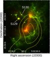 |
Fig. 1 WISE two-color image of H II region Sh2-236 and the cometary globules S129 and S130 at 12 μm in green, and22 μm in red. The yellow contours represent the 12CO (1–0) emission (angular resolution about 3.75 arcmin) integrated between − 10 and + 10 km s−1 extracted from the CfA 1.2 m CO Survey Archive (Dame et al. 2001). Contour levels are at 3, 4, and 5 K km s−1. The systemic velocity of the CO emission is about −7 km s−1. |
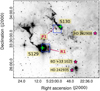 |
Fig. 2 Spitzer-IRAC emission at 5.8 μm of S129 and S130. The grayscale goes from 3 to 9 MJy sr−1. P1 and R1 indicate the position of a pillar-like feature and a region of diffuse gas, respectively. The blue squares indicate the regions mapped in 12CO J = 3−2 and HCO+ J = 4−3 lines. The green crosses represent the location of the single pointings of the HCO+, HCN, HNC J = 4−3, and C2 H N = 4−3 J = 9/2–7/2 lines. |
Ionizing stars of S129 and S130.
2 Molecular observations and data reduction
The observation of the molecular lines was carried out on October 3, 4, and 5, 2016 with the 10 m Atacama Submillimeter Telescope Experiment (ASTE, Ezawa et al. 2004). We used the DASH 345 GHz band receiver, which is a cartridge-type dual-polarization side-band separating (2SB) mixer receiver for 350 GHz band remotely tunable in the LO frequency range of 330–366 GHz. We simultaneously observed 12CO J = 3−2 at 345.79 GHz and HCO+ J = 4−3 at 356.734 GHz, mapping two regions of about 1′ × 1′ centered at RA = 05:23:06; Dec = +33:28:37 and RA = 05:22:58; Dec = +33:31:35 (J2000) (blue squares in Fig. 2), which mainly include the CGs S129 and S130, respectively, and other interesting nearby structures. The mapping grid spacing was 20′′, and the integration time was 60 s per pointing. We also performed two single pointings centered at RA = 05:23:08; Dec = +33:28:31, and RA = 05:22:55; Dec = +33:31:40 (J2000) (green crosses in Fig. 2) of C2H N = 4−3 at 349.34 GHz, and HNC J = 4−3 at 362.63 GHz simultaneously, and HCN J = 4−3 at 354.50 GHz with an integration time of about 30 min per pointing. Table 2 indicates whether the observed molecule was detected or not.
The observations were performed in position-switching mode. We used the XF digital spectrometer MAC with a bandwidth and spectral resolution set to 128 MHz and 125 kHz, respectively. The velocity resolution is 0.11 km s−1, and the beam size (FWHM) is 22′′ at 350 GHz. The system temperature varied from about Tsys = 150 to 250 K during the observations. The main beam efficiency was ηmb ~ 0.65. The data were reduced with NEWSTAR1 and the spectra processed using the XSpec software package2. The baseline fitting was done using second-order polynomials for all lines. The HCO+, HCN, HNC, and C2H J = 4−3 spectra were Hanning-smoothed to improve the signal-to-noise ratio. The resulting spectral resolution of the observations was about 0.4 km s−1. The rms noise level was about 100 mK for 12CO J = 3−2, and HCO+ J = 4−3 transitions, and about 30 mK for the rest of the molecules.
Molecules observed with ASTE.
3 Results
In the following section, we present the results derived from the analysis of our molecular observations complemented with public multiwavelength data.
3.1 Description of the infrared and optical emission
Figure 2 shows a zoom-up view of the region containing S129 and S130 as seen at 5.8 μm extracted from the Spitzer/GLIMPSE Survey (Benjamin et al. 2003; Churchwell et al. 2009). The green crosses indicate the positions of the single pointings observations of the HCN and HNC J = 4−3 and C2H N = 4−3 J = 9/2–7/2 line. The blue squares indicate the regions mapped in the 12CO J = 3−2 and HCO+ J = 4−3 transitions. These regions include S129 and S130, but also two striking structures, which are presented for the first time in this work. The first one is a small pillar-like feature that appears in projection close to S130 (P1in Fig. 2). The second one can be appreciated as the diffuse emission at 5.8 μm (R1 in Fig. 2), which is located, in projection, in front of the head of S129.
The central panel of Fig. 3 shows the optical emission toward S129 and S130 extracted from the Digital Sky Survey3. Both CGs exhibit conspicuous bright rims (BRs) facing the location of the ionizing stars. The orientation of the BR related to S130 suggests that the star HD 242908 is the main one responsible for ionizing the globule. In particular, toward S129 a striking nebulosity located, in projection, at the interior of the globule can be seen. This nebulosity could be associated with the young stars cluster found by Maheswar et al. (2007). In Fig. 3, the left and right panels show the Ks band emission extracted from UKIDSS survey4 toward S129and S130, respectively. The green contours represent the radio continuum emission at 1.4 GHz obtained from the NVSS5 which traces the ionized gas associated with the CGs. Despite the relatively low angular resolution of the survey (~ 45′′), its positional uncertainty of about 1 arcsec allows us to conclude that the peak of the radio continuum emission related to S129 coincides with the position of the over-density of stars likely embedded in the globule, suggesting that some of these young stars have begun to ionize the inner gas of S129. However, we can not discard a contribution of the ionized boundary layer to the radio continuum emission toward this globule. On the other hand, the radio continuum emission associated with S130 seems to peak at the brightest border of the globule, which suggests that this emission mostly arises from its ionized boundary layer. The elongated morphology of the radio continuum emission toward S130 is consistent with a globular cometary shape, reinforcing the scenario in which the ionized gas is related to the action of external sources.
3.2 The molecular gas
3.2.1 12CO J = 3−2 spectra
Figure 4 shows the 12CO J = 3−2 spectra obtained with ASTE toward S129 (bottom panel) and the region where these spectra were taken (green squares and crosses) superimposed on the Spitzer-IRAC 5.8 μm emission (top panel). The black contours represent the submillimeter continuum emission at 850 μm from the Submillimeter Common-User Bolometer Array (SCUBA; Di Francesco et al. 2008) extracted from the James Clerk Maxwell Telescope (JCMT) data archive6. The SCUBA sources JCMTS J052308.4+332837 and JCMTS J052304.1+332813, cataloged by Di Francesco et al. (2008), positionally coincide with the head of S129 and with the region of diffuse gas identified as R1 in Fig. 2, respectively. The mapped region of about 1′ × 1′ partially covers the location of both SCUBA sources, which seem to be connected in projection. Toward the (−20, 0) offset the spectrum shows two velocity components centered at about −2.6 and at −0.9 km s−1. These components also appear toward other offsets, but weaker. As we move from the head of S129 toward R1, a third velocity component appears centered at about +10.2 km s−1. This component is more intense at the (+20, −20) offset, which suggests that it corresponds to molecular gas related to R1. Toward the (0, 0) offset, the spectrum shows three velocity components centered at about −2.5, −0.7 (the same that at the (−20, 0) offset), and +10.2 km s−1 (likely related to R1 feature).
Table 3 presents the parameters derived from the Gaussian fittings to the spectra at the (−20, 0) and (0, 0) offsets, meaning the positions that coincide with S129 head.
Figure 5 shows the 12CO J = 3−2 spectra obtained with ASTE toward S130 (bottom panel) and the region where these spectra were taken (green squares and crosses) superimposed on the Spitzer-IRAC 5.8 μm emission (top panel). The mappedregion of about 1′ × 1′ partially covers the head of S130 and the small pillar-like feature, P1. The spectra at the (+20, +20) and (+20, 0) offsets, which were taken in positional coincidence with S130, show a velocity component centered at about −11 km s−1. This component corresponds to molecular gas associated with the CG. On the other hand, the spectrum at the (−20, +20) offset shows a velocity component centered at about +4 km s−1. This component is also present at the (0, +20), (−20, 0), and (0, 0) offsets, but weaker. Given the positions of these spectra, this velocity component would correspond to molecular gas associated with the small pillar-like feature P1.
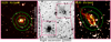 |
Fig. 3 Central panel: optical emission extracted from the Digital Sky Survey 2 (DSS2) toward S129 and S130. Left-panel: zoom-up view of S129 at the UKIDSS Ks band. Right-panel: zoom-up view of S130 at the UKIDSS Ks band. Green contours represent the radio continuum emission at 1.4 GHz extracted from the NRAO VLA Sky Survey (NVSS; Condon et al. 1998). Levels are at 5, 10, and 15 mJy beam−1. Radio continuum shows the NVSS sources 052307+332832 and 052255+333156 related to S129 and S130, respectively. |
3.2.2 High-density molecular gas tracers
The HCO+ molecule was only detected toward S130. Figure 6 shows the HCO+ J = 4−3 spectra, which were taken toward the same region as the 12CO spectra (seeFig. 5). The same two velocity components that were observed in the 12CO spectra at −11 km s−1 (S130) andat +4 km s−1 (P1) can be appreciated.
Figure 7 shows the HCN J = 4−3 (upper panel) and HNC J = 4−3 (lower panel) spectra obtained toward the head of S130 (green cross at the S130 position in Fig. 2). Both lines show the same velocity component centered at about −11 km s−1 as seen in the 12CO line toward the (+20, +20) and (+20, 0) offsets (see Fig. 5). The parameters obtained from Gaussian fittings are listed in Table 4. The HCN/HNC integrated ratio is about three. HCN and HNC were not detected in S129.
3.2.3 C2H molecule: a photo-dissociation region tracer
The C2H was the only molecule, with the exception of 12CO, detected toward both CGs. Figure 8 shows the C2H N = 4−3 J = 9/2–7/2 spectra obtained toward S129 and S130 (green crosses in Fig. 2). The spectrum obtained toward S129 shows two velocity components centered at about −3.6 and −0.8 kms−1. The shape of the profile is similar to that of the 12CO J = 3−2 at the (−20, 0) offset toward S129, but the central velocity of the blue-shifted components differs in 1 km s−1. The C2 H spectrum obtained toward S130 exhibits just one velocity component centered at about −11 km s−1, which corresponds to the same component detected in the 12CO J = 3−2 and HCO+ J = 4–3 at the (+20, +20) offset. The Gaussian fit parameters are listed in Table 4.
4 Discussion
In this section we discuss the more relevant spectral features presented above in order to: (1) unveil the nature of each individual object, and (2) disentangle the spatial distribution of the sources in the context of Sh2–236.
4.1 Infall signatures and molecular outflows in S129
An analysis of the molecular line profiles may help us to identify kinematic signatures associated with different dynamic processes that could be occurring in the interior of the molecular clouds, such as outflows, rotation, expansion, and infall. The inward motion of gas caused by gravity in regions of star formation, for instance, may lead to a self-absorbed emission line profile of an optically-thick line. Simple early models (see, e.g., Myers et al. 1996, and references therein) predict a “blue asymmetry” where the blue peak in the double-peak profile becomes brighter than the red one. Several studies found observational evidence supporting this model (e.g., Lee et al. 2004; Tsamis et al. 2008; Stahler & Yen 2010).
Figure 9 shows the 12CO J = 3−2 spectra toward S129 at the (−20, 0) and (0, 0) offsets. The blue component appears more intense than the red one, which may imply infall motions of the gas. The C2 H J = 4−3 spectrum toward the head of S129 shows the same “blue-skewed” profile (see Fig. 8). Thus, it is likely that the “dip” observed at −1.5 and at −2 km s−1 in the 12CO and C2 H profiles, respectively, is a self-absorption feature. Moreover, Lim et al. (2018) detected hydrogen molecular gas toward S129 with a velocity component at about −1.5 kms−1, which supports the “dip” interpretation of the profiles, and reinforces the scenario of infall gas motion in the CG.
On the other hand, the 12CO J = 3−2 spectrum presented in Fig. 9 shows evidence of turbulent gas. A red-wing at the (0, 0) offset is visible, likely related to the molecular outflow activity generated by the young stars that are forming inside S129.
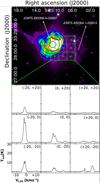 |
Fig. 4 12CO J = 3−2 spectra toward the region of S129. The region where the spectra were taken is shown superimposed on the Spitzer-IRAC 5.8 μm emission. The color scale goes from 10 MJy sr−1 (violet) to 60 MJy sr−1 (white). The black contours represent the submillimeter continuum emission at 850 μm as extracted from the SCUBA survey. The levels are at 40, 70, 100, 120, 180, and 250 mJy beam−1. |
4.2 Analyzing the high-density gas in the globules
We only detected HCO+ J = 4−3 toward the region of S130. The results showed in Sect. 3.1 suggest that, despite the low angular resolution of the NVSS data, the ionized gas related to S129 seems to have two contributions: one from the ionized boundary layer, and other one from the activity of young stars embedded in the globule, while most of the ionized gas associated with S130 seems to arise from the illuminated border of the globule. Goicoechea et al. (2009) found a decrease of the HCO+ abundance from the shielded core to the UV irradiated cloud edge in the Horsehead nebula. The authors attributed this diminishing of the HCO+ abundance to the electronic recombination, which becomes more significant as the number of free electrons increases. The angular resolution of our molecular observations does not allow us to discern whether the HCO+ emission arises from the interior of the globule or from the irradiated border of the cloud. However, it is likely that the HCO+ emission detected toward S130 comes from the neutral gas of its interior, while the non-detection of HCO+ toward S129 could be explained by the presence of ionized gas at both the interior and the edge of the globule. This points to different star-forming evolutionary stages between both globules (Sanhueza et al. 2012; Hoq et al. 2013).
The HCN and HNC molecules are also high-density gas tracers. As in the case of HCO+, we only detected HCN and HNC J = 4−3 lines toward S130. Graninger et al. (2014) suggested that the HCN/HNC abundance ratio can be used to trace the evolutionary stages of star-forming regions. Jin et al. (2015) found a statistically increasing tendency of the abundance ratio with the evolution of the objects, with values that go from about one in the starless clumps to about nine in the UCH II regions. According to the authors, this may be due to a temperature increase that favors the reaction: HNC + H → HCN + H. In addition, Chenel et al. (2016) and Aguado et al. (2017) showed that in the interstellar regions exposed to intense UV radiation fields, HCN should be more abundant than HNC. They showed that the destruction of both isomers is dominated by the photodissociation, and the HNC is destroyed faster than the HCN. Taking into account these results and assuming similar excitation conditions for both isomers toward the head of S130, which is a quite-likely assumption, the integrated ratio of about three derived in Sect. 3.2.2 is in agreement with a scenario of incipient star formation, where the young stars are not ionizing the interior of the globule. On the other hand, the non-detection of both isomers toward S129 could be due to a low abundance (emission undetectable for the ASTE sensitivity), or to both isomers being destroyed by the radiation field from the likely cluster of young stars within this globule as seen in the Ks band (Fig. 3 left).
Finally, the C2H N = 4−3 J = 9/2–7/2 line was detected toward S129 and S130. It is well known that the C2H molecule is a photo-dissociation regions (PDRs) tracer (Fuente et al. 1993, 1996; Jansen et al. 1995; Nagy et al. 2015). The PDR is the transition layer between the ionized gas directly irradiated by strong UV fields (e.g., from massive OB stars) and the cold neutral gas shielded from radiation (e.g. Tielens & Hollenbach 1985). Tielens (2013) present one of the most complete studies of the chemistry of this molecule involved in the PDRs.
The C2H N = 4−3 J = 9/2–7/2 toward S129 exhibits a similar blue-skewed spectrum as the 12CO spectra toward the (−20, 0) and (0, 0) offsets, supporting the interpretation of infall motions of the gas as was previously discussed. We suggest that while the HCO+, HCN, and HNC molecules exhibit the differences between the internal conditions of the gas of S129 and S130, the ubiquitous presence of the C2H molecule toward both globules shows that the nearby O-B stars are irradiating the external layers of S129 and S130.
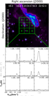 |
Fig. 5 12CO J = 3−2 spectra toward the region of S130. The region where the spectra were taken is shown superimposed on the Spitzer-IRAC 5.8 μm emission. The color scale goes from 10 MJy sr−1 (violet) to 50 MJy sr−1 (green). |
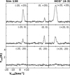 |
Fig. 6 HCO+ J = 4−3 spectra toward the region of S130. The region where the spectra were taken is the same as shown in Fig. 5. |
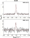 |
Fig. 7 HCN J = 4−3 (upper panel) and HNC J = 4−3 (lower panel) spectra toward S130. The spectra were obtained toward the position of the green cross shown in Fig. 2. The red curves correspond to Gaussian fittings. The derived parameters are shown in Table 4. |
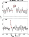 |
Fig. 8 C2H N = 4−3 J = 9/2–7/2 spectra toward S129 (upper panel) and S130 (lower panel). The spectra were obtained toward the positions of the green crosses shown in Fig. 2. The red curves correspond to Gaussian fittings. The derived parameters are shown in Table 4. The dashed vertical green line indicates the RV for the H2 1−0 S(1) line related to S129 found by Lim et al. (2018). |
4.3 Schematic view of the molecular features in the context of Sh2–236
Based on spectroscopic optical observations, Lim et al. (2018) found a bimodal distribution in RV of the stars in the region. The main peak is at −3.9 kms−1 and corresponds to the systemic velocity of NGC 1893. The secondary peak corresponds to a second subgroup of young stars at +2.6 km s−1. The authors also found a bimodal behavior in the RV of the ionized gas. From the forbidden line N II (λ6584), they observed two velocity components at −13 and +4.2 km s−1, which correspond to the near and far side, respectively, of a bubble with an expansion velocity of about 8.6 km s−1. Finally, based on spectroscopic observationsof the near-infrared H2 1−0 S(1) line, they found RVs of about −1.5 and −11 km s−1 for the hot molecular gas related to S129 and S130, respectively.
Based on our observations, we found similar RV components of the cold molecular gas associated with S129 and S130 (see Table 5), supporting that S129 and S130 should be located at the far and the near side of the shell, respectively. Additionally, the molecular gas related to the small pillar-like feature P1 has an RV of +4 kms−1, which is exactly the same RV of the far side of the shell of the expanding bubble.
Finally,the RV of the molecular gas related to R1 (about +10 km s−1) differs in more than 11 km s−1 with the RVof S129, which suggests that while S129 is located at the far side of the expanding shell, R1 would be placed well beyond.
Radial velocities of gas associated with the four molecular structures characterized in this work.
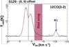 |
Fig. 9 12CO J = 3−2 spectrum toward S129 at the (0, 0) offset. The red curve corresponds to the Gaussian fitting. The dashed vertical blue line indicates the RV for the H2 1−0 S(1) line related to S129 found by Lim et al. (2018). |
5 Summary
In the literature, there are several studies about the cometary globules S129 and S130 in Sh2−236, but, with the exception of Lim et al. (2018), they focused on the stellar content. Therefore, for a complete understanding of the processes that are occurring in the region, a study of the molecular gas associated with globules was needed, and thus we present a kinematic study of the molecular gas associated with S129 and S130 and their environments. The main results are summarized as follows.
We find kinematic signatures of infalling gas in the 12CO J = 3−2 and C2H N = 4−3 J = 9/2–7/2 spectra toward S129. We detect HCO+, HCN, and HNC J = 4−3 only toward S130. The integrated ratio of HCN/HNC of about three is in agreement with a scenario of incipient star formation where the young stars are not ionizing the interior of the globule. The non-detection of these molecules toward S129 could be due to the radiation field arising from the star-formation activity inside this globule. The ubiquitous presence of the C2 H molecule toward S129 and S130 evidences the action of the nearby O-B stars irradiating the external layer of both globules.
Based on the mid-infrared 5.8 μm emission, we identify two new structures: (1) a region of diffuse emission (R1) located in front of the head of S129 and (2) a pillar-like feature (P1) placed beside S130. Based on the 12CO J = 3−2 line, we find molecular gas associated with S129, S130, R1 and P1 at radial velocities of −1.5, −11, +10, and +4 km s−1, respectively. Therefore, while S129 and P1 are located at the far side of the shell, S130 is placed at the near side.
Finally, the RV of the molecular gas related to R1 differs in more than 11 km s−1 with the RV of S129, which suggests that while S129 is located at the far side of the expanding shell, R1 would be placed well beyond.
Acknowledgements
We thank the anonymous referee for her/his fruitful comments. The ASTE project is led by Nobeyama Radio Observatory (NRO), a branch of National Astronomical Observatory of Japan (NAOJ), in collaboration with University of Chile, and Japanese institutes including University of Tokyo, Nagoya University, Osaka Prefecture University, Ibaraki University, Hokkaido University, and the Joetsu University of Education. M.O. and S.P. are members of the Carrera del investigador científico of CONICET, Argentina. M.B.A. is a doctoral fellow of CONICET, Argentina. This work was partially supported by grants awarded by ANPCYT and UBA (UBACyT) from Argentina. M.R. wishes to acknowledge support from FONDECYT(CHILE) grant No 1140839. M.O. is grateful to Dr. Natsuko Izumi for the support received during the ASTE observations.
References
- Aguado, A., Roncero, O., Zanchet, A., Agúndez, M., & Cernicharo, J. 2017, ApJ, 838, 33 [NASA ADS] [CrossRef] [Google Scholar]
- Avedisova, V. S., & Kondratenko, G. I. 1984, Nauchnye Informatsii, 56, 59 [NASA ADS] [Google Scholar]
- Benjamin, R. A., Churchwell, E., Babler, B. L., et al. 2003, PASP, 115, 953 [NASA ADS] [CrossRef] [Google Scholar]
- Bertoldi, F. 1989, ApJ, 346, 735 [NASA ADS] [CrossRef] [Google Scholar]
- Bisbas, T. G., Wünsch, R., Whitworth, A. P., Hubber, D. A., & Walch, S. 2011, ApJ, 736, 142 [Google Scholar]
- Blitz, L., Fich, M., & Stark, A. A. 1982, ApJS, 49, 183 [NASA ADS] [CrossRef] [Google Scholar]
- Cerqueira, A. H., Cantó, J., Raga, A. C., & Vasconcelos, M. J. 2006, Rev. Mex. Astron. Astrofis., 42, 203 [NASA ADS] [Google Scholar]
- Chenel, A., Roncero, O., Aguado, A., Agúndez, M., & Cernicharo, J. 2016, J. Chem. Phys., 144, 144306 [NASA ADS] [CrossRef] [Google Scholar]
- Churchwell, E., Babler, B. L., Meade, M. R., et al. 2009, PASP, 121, 213 [NASA ADS] [CrossRef] [Google Scholar]
- Condon, J. J., Cotton, W. D., Greisen, E. W., et al. 1998, AJ, 115, 1693 [NASA ADS] [CrossRef] [Google Scholar]
- Dame, T. M., Hartmann, D., & Thaddeus, P. 2001, ApJ, 547, 792 [NASA ADS] [CrossRef] [Google Scholar]
- Di Francesco, J., Johnstone, D., Kirk, H., MacKenzie, T., & Ledwosinska, E. 2008, ApJS, 175, 277 [NASA ADS] [CrossRef] [Google Scholar]
- Elmegreen, B. G., & Lada, C. J. 1977, ApJ, 214, 725 [NASA ADS] [CrossRef] [Google Scholar]
- Ezawa, H., Kawabe, R., Kohno, K., & Yamamoto, S. 2004, Proc. SPIE, 5489, 763 [NASA ADS] [CrossRef] [Google Scholar]
- Fuente, A., Martin-Pintado, J., Cernicharo, J., & Bachiller, R. 1993, A&A, 276, 473 [NASA ADS] [Google Scholar]
- Fuente, A., Rodriguez-Franco, A., & Martin-Pintado, J. 1996, A&A, 312, 599 [NASA ADS] [Google Scholar]
- Goicoechea, J. R., Pety, J., Gerin, M., Hily-Blant, P., & Le Bourlot, J. 2009, A&A, 498, 771 [NASA ADS] [CrossRef] [EDP Sciences] [Google Scholar]
- Graninger, D. M., Herbst, E., Öberg, K. I., & Vasyunin, A. I. 2014, ApJ, 787, 74 [NASA ADS] [CrossRef] [Google Scholar]
- Gritschneder, M., Burkert, A., Naab, T., & Walch, S. 2010, ApJ, 723, 971 [NASA ADS] [CrossRef] [Google Scholar]
- Hoq, S., Jackson, J. M., Foster, J. B., et al. 2013, ApJ, 777, 157 [NASA ADS] [CrossRef] [Google Scholar]
- Jansen, D. J., Spaans, M., Hogerheijde, M. R., & van Dishoeck, E. F. 1995, A&A, 303, 541 [NASA ADS] [Google Scholar]
- Jin, M., Lee, J.-E., & Kim, K.-T. 2015, ApJS, 219, 2 [NASA ADS] [CrossRef] [Google Scholar]
- Lee, C. W., Myers, P. C., & Plume, R. 2004, ApJS, 153, 523 [NASA ADS] [CrossRef] [Google Scholar]
- Lefloch, B., & Lazareff, B. 1994, A&A, 289, 559 [NASA ADS] [Google Scholar]
- Lim, B., Sung, H., Bessell, M. S., et al. 2018, MNRAS, 477, 1993 [NASA ADS] [CrossRef] [Google Scholar]
- Mackey, J., & Lim, A. J. 2010, MNRAS, 403, 714 [NASA ADS] [CrossRef] [Google Scholar]
- Maheswar, G., Sharma, S., Biman, J. M., Pandey, A. K., & Bhatt, H. C. 2007, MNRAS, 379, 1237 [NASA ADS] [CrossRef] [Google Scholar]
- Marco, A., & Negueruela, I. 2002, A&A, 393, 195 [NASA ADS] [CrossRef] [EDP Sciences] [Google Scholar]
- Myers, P. C., Mardones, D., Tafalla, M., Williams, J. P., & Wilner, D. J. 1996, ApJ, 465, L133 [NASA ADS] [CrossRef] [Google Scholar]
- Nagy, Z., Ossenkopf, V., Van der Tak, F. F. S., et al. 2015, A&A, 578, A124 [NASA ADS] [CrossRef] [EDP Sciences] [Google Scholar]
- Negueruela, I., Marco, A., Israel, G. L., & Bernabeu, G. 2007, A&A, 471, 485 [NASA ADS] [CrossRef] [EDP Sciences] [Google Scholar]
- Sandford, II, M. T., Whitaker, R. W., & Klein, R. I. 1982, ApJ, 260, 183 [NASA ADS] [CrossRef] [Google Scholar]
- Sanhueza, P., Jackson, J. M., Foster, J. B., et al. 2012, ApJ, 756, 60 [NASA ADS] [CrossRef] [Google Scholar]
- Sharpless, S. 1959, ApJS, 4, 257 [Google Scholar]
- Sota, A., Maíz Apellániz, J., Morrell, N. I., et al. 2014, ApJS, 211, 10 [NASA ADS] [CrossRef] [Google Scholar]
- Stahler, S. W., & Yen, J. J. 2010, MNRAS, 407, 2434 [NASA ADS] [CrossRef] [Google Scholar]
- Tielens, A. G. G. M. 2013, Rev. Mod. Phys., 85, 1021 [NASA ADS] [CrossRef] [Google Scholar]
- Tielens, A. G. G. M., & Hollenbach, D. 1985, ApJ, 291, 722 [NASA ADS] [CrossRef] [Google Scholar]
- Tremblin, P., Audit, E., Minier, V., Schmidt, W., & Schneider, N. 2012a, A&A, 546, A33 [NASA ADS] [CrossRef] [EDP Sciences] [Google Scholar]
- Tremblin, P., Audit, E., Minier, V., & Schneider, N. 2012b, A&A, 538, A31 [NASA ADS] [CrossRef] [EDP Sciences] [Google Scholar]
- Tsamis, Y. G., Rawlings, J. M. C., Yates, J. A., & Viti, S. 2008, MNRAS, 388, 898 [NASA ADS] [CrossRef] [Google Scholar]
- Walch, S., Whitworth, A. P., Bisbas, T. G., Wünsch, R., & Hubber, D. A. 2013, MNRAS, 435, 917 [NASA ADS] [CrossRef] [Google Scholar]
Reduction software based on AIPS developed at NRAO, extended to treat single-dish data with a graphical user interface (GUI).
XSpec is a spectral line-reduction package for astronomy, which has been developed by Per Bergman at Onsala Space Observatory.
All Tables
Radial velocities of gas associated with the four molecular structures characterized in this work.
All Figures
|
Fig. 1 WISE two-color image of H II region Sh2-236 and the cometary globules S129 and S130 at 12 μm in green, and22 μm in red. The yellow contours represent the 12CO (1–0) emission (angular resolution about 3.75 arcmin) integrated between − 10 and + 10 km s−1 extracted from the CfA 1.2 m CO Survey Archive (Dame et al. 2001). Contour levels are at 3, 4, and 5 K km s−1. The systemic velocity of the CO emission is about −7 km s−1. |
| In the text | |
|
Fig. 2 Spitzer-IRAC emission at 5.8 μm of S129 and S130. The grayscale goes from 3 to 9 MJy sr−1. P1 and R1 indicate the position of a pillar-like feature and a region of diffuse gas, respectively. The blue squares indicate the regions mapped in 12CO J = 3−2 and HCO+ J = 4−3 lines. The green crosses represent the location of the single pointings of the HCO+, HCN, HNC J = 4−3, and C2 H N = 4−3 J = 9/2–7/2 lines. |
| In the text | |
|
Fig. 3 Central panel: optical emission extracted from the Digital Sky Survey 2 (DSS2) toward S129 and S130. Left-panel: zoom-up view of S129 at the UKIDSS Ks band. Right-panel: zoom-up view of S130 at the UKIDSS Ks band. Green contours represent the radio continuum emission at 1.4 GHz extracted from the NRAO VLA Sky Survey (NVSS; Condon et al. 1998). Levels are at 5, 10, and 15 mJy beam−1. Radio continuum shows the NVSS sources 052307+332832 and 052255+333156 related to S129 and S130, respectively. |
| In the text | |
|
Fig. 4 12CO J = 3−2 spectra toward the region of S129. The region where the spectra were taken is shown superimposed on the Spitzer-IRAC 5.8 μm emission. The color scale goes from 10 MJy sr−1 (violet) to 60 MJy sr−1 (white). The black contours represent the submillimeter continuum emission at 850 μm as extracted from the SCUBA survey. The levels are at 40, 70, 100, 120, 180, and 250 mJy beam−1. |
| In the text | |
|
Fig. 5 12CO J = 3−2 spectra toward the region of S130. The region where the spectra were taken is shown superimposed on the Spitzer-IRAC 5.8 μm emission. The color scale goes from 10 MJy sr−1 (violet) to 50 MJy sr−1 (green). |
| In the text | |
|
Fig. 6 HCO+ J = 4−3 spectra toward the region of S130. The region where the spectra were taken is the same as shown in Fig. 5. |
| In the text | |
|
Fig. 7 HCN J = 4−3 (upper panel) and HNC J = 4−3 (lower panel) spectra toward S130. The spectra were obtained toward the position of the green cross shown in Fig. 2. The red curves correspond to Gaussian fittings. The derived parameters are shown in Table 4. |
| In the text | |
|
Fig. 8 C2H N = 4−3 J = 9/2–7/2 spectra toward S129 (upper panel) and S130 (lower panel). The spectra were obtained toward the positions of the green crosses shown in Fig. 2. The red curves correspond to Gaussian fittings. The derived parameters are shown in Table 4. The dashed vertical green line indicates the RV for the H2 1−0 S(1) line related to S129 found by Lim et al. (2018). |
| In the text | |
|
Fig. 9 12CO J = 3−2 spectrum toward S129 at the (0, 0) offset. The red curve corresponds to the Gaussian fitting. The dashed vertical blue line indicates the RV for the H2 1−0 S(1) line related to S129 found by Lim et al. (2018). |
| In the text | |
Current usage metrics show cumulative count of Article Views (full-text article views including HTML views, PDF and ePub downloads, according to the available data) and Abstracts Views on Vision4Press platform.
Data correspond to usage on the plateform after 2015. The current usage metrics is available 48-96 hours after online publication and is updated daily on week days.
Initial download of the metrics may take a while.