| Issue |
A&A
Volume 632, December 2019
|
|
|---|---|---|
| Article Number | A22 | |
| Number of page(s) | 6 | |
| Section | Numerical methods and codes | |
| DOI | https://doi.org/10.1051/0004-6361/201936487 | |
| Published online | 21 November 2019 | |
PreProFit: Pressure Profile Fitter for galaxy clusters
INAF-Osservatorio Astronomico di Brera, via Brera 28, 20121 Milano, Italy
e-mail: This email address is being protected from spambots. You need JavaScript enabled to view it.
Received:
9
August
2019
Accepted:
19
September
2019
Abstract
Galaxy cluster analyses based on high-resolution observations of the Sunyaev–Zeldovich (SZ) effect have become common in the last decade. We present PreProFit, the first publicly available code designed to fit the pressure profile of galaxy clusters from SZ data. PreProFit is based on a Bayesian forward-modelling approach, allows the analysis of data coming from different sources, adopts a flexible parametrization for the pressure profile, and fits the model to the data accounting for Abel integral, beam smearing, and transfer function filtering. PreProFit is computationally efficient, is extensively documented, has been released as an open source Python project, and was developed to be part of a joint analysis of X-ray and SZ data on galaxy clusters. PreProFit returns χ2, model parameters and uncertainties, marginal and joint probability contours, diagnostic plots, and surface brightness radial profiles. PreProFit also allows the use of analytic approximations for the beam and transfer functions useful for feasibility studies.
Key words: methods: data analysis / methods: numerical / methods: statistical / galaxies: clusters: intracluster medium / cosmic background radiation
© ESO 2019
1. Introduction
Galaxy clusters are the largest and most massive gravitationally bound objects in the Universe, and thus they offer a unique tracer of cosmic evolution. The thermodynamic properties of a galaxy cluster can be gathered from observation in the optical band, the X-ray band, or microwaves. The hot gas trapped in the cluster’s gravitational potential leaves an imprint on the microwave sky because its electrons Compton scatter the photons of the cosmic microwave background radiation (Sunyaev & Zeldovich 1970, 1972). The distortion is best observable at millimetre wavelengths and is directly proportional to the pressure distribution in the clusters. Specifically, the amplitude of the SZ effect is parametrized as the Compton y parameter.
The number of high-resolution SZ instruments has progressively increased throughout the last decade, including the NIKA1 camera (Monfardini et al. 2010) and the GISMO2 camera (Staguhn et al. 2008) at the IRAM3 30m telescope, the MUSTANG4 camera (Dicker et al. 2008) on the 100 m Robert C. Byrd Green Bank Telescope, the Planck satellite (Planck Collaboration Int. V 2013), the Bolocam array (Czakon et al. 2015) and the MUSIC5 camera (Sayers et al. 2019) on the Caltech Sub-millimeter Observatory, and the ALMA6+ACA7 and CARMA8 (Woody et al. 2004) arrays. Furthermore, a new generation of instruments such as NIKA2 (Calvo et al. 2016), MUSTANG2 (Dicker et al. 2014), and TolTEC (Austermann et al. 2018) have recently been developed, which have improved the quality and quantity of SZ data.
Several studies on the SZ effect have been performed (e.g. Birkinshaw et al. 2005; Mroczkowski et al. 2009; Korngut et al. 2011; Sayers et al. 2013; Adam et al. 2015; Romero et al. 2017) and the methodologies for operating with these data are constantly evolving. In most cases, the SZ data analysis improves in order to meet the specific demands of each analysis (e.g. using the actual beam in place of a Gaussian approximation of it).
In this paper, we present PreProFit, which is, to the best of our knowledge, the first publicly available code for fitting the pressure profile of galaxy clusters. PreProFit is meant to automate and generalize all the phases of data analyses in an efficient and easy-to-use software pipeline, and therein lies its most remarkable feature.
PreProFit includes highly time-consuming operations such as convolutions. As a result, our purpose throughout the software development was to find a way to perform these tasks sufficiently quickly, but without losing accuracy. PreProFit is able to analyse data coming from different sources and also allows the use of analytic approximations for the beam and transfer functions, useful for feasibility studies, or to make use of published data with only approximate information on theses quantities. PreProFit has been developed to be part of a joint analysis of X-ray and SZ data on galaxy clusters.
The paper is organised as follows: in Sect. 2 we provide an overview of the software, as well as the technical requirements; in Sect. 3 we describe in detail the methodology behind each step of the program; and in Sect. 4 we present an application of PreProFit on real data from the galaxy cluster CL J1226.9+3332. We conclude with the discussion and final remarks in Sect. 5.
2. PreProFit
2.1. Program flow
PreProFit adopts a flexible parametrization for the pressure profile of the cluster and properly derives the surface brightness profile to be compared with the observed data. It assumes spherical symmetry for the cluster, as in most analyses (e.g. Comis et al. 2011; Adam et al. 2015; Romero et al. 2015, 2017). As outlined in Fig. 1, PreProFit projects the three-dimensional pressure profile into a two-dimensional map using the forward Abel transform. The map is then convolved with the instrumental beam and the transfer function. With opportune conversion factors, we finally derive the surface brightness profile, whose fit to the data is measured through the likelihood function of the model. PreProFit automatically produces a number of diagnostic plots, including the model and data radial surface brightness profile.
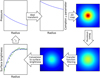 |
Fig. 1. Block diagram showing the program flow. |
2.2. Requirements and installation
PreProFit was developed and tested with Python 3.6. The following libraries were required to build: mbproj2, PyAbel, numpy, scipy, astropy, emcee, six, matplotlib, corner. PreProFit can be downloaded from GitHub9.
3. Methods
3.1. Key stages
To follow, we present a step by step description of PreProFit working principles, as illustrated in Fig. 1.
3.1.1. Pressure profile
The pressure profile is described by the generalized Navarro, Frenk & White (gNFW) model proposed by Nagai et al. (2007):
 (1)
(1)
where P0 is a normalizing constant and rp is a scale radius. The exponentials b and c describe the logarithmic slopes at r/rp ≫ 1 and r/rp ≪ 1, respectively, while a governs the rate of turnover between these two slopes. The five parameters make the model very flexible; they can fit current data and allow users to identify which parameters are constrained by the data.
3.1.2. Abel integral
The three-dimensional pressure model is numerically integrated along the line of sight in order to obtain a two-dimensional map of the Compton y parameter. This is performed according to the Abel transform:
 (2)
(2)
where σT is the electron Thompson scattering cross section, me is the electron rest mass, c is the speed of light, and Rb is the cluster radial extent. To calculate the integral, PreProFit makes use of the well-developed Python function direct_transform from the PyAbel library.
At this stage, we create a two-dimensional map for the Compton y parameter profile adopting a regular grid and complying with radial symmetry.
3.1.3. Beam smearing
In order to consider the effects of the instrument used for observing the cluster, we need to convolve our model map with the beam. PreProFit supports either to read the beam data from a file or to approximate it with a Gaussian distribution (e.g. based on the instrumental full width at half maximum) when, for example, these data are not available. By default, the beam map is normalized to have an integral of one, but it can even be left as such on user request. The convolution is performed via fast Fourier transform (FFT).
3.1.4. Transfer function
After convolving with the beam, the input transfer function10 is applied to the model in the Fourier space. If requested, PreProFit allows the use of an approximation based on the cumulative distribution function of a Gaussian with location, scale, and normalization parameters chosen by the user. From the radial transfer function profile, we construct a two-dimensional transmission image assuming radial symmetry. To pass our model through the signal transfer function, we multiply the unfiltered map in the Fourier space with the transmission image just created. Compared to implementations in Adam et al. (2015) and Romero et al. (2017), PreProFit adopts a more general approach for the transfer function filtering allowing free values for the image pixel size and the transfer function sampling step.
3.1.5. Conversion to surface brightness
To compare our model map with the observed data, the filtered Compton y parameter map is converted into surface brightness, measured in Jy beam−1, using the input conversion factor.
3.2. Model definition
The whole set of operations described in the previous sections represents our model, which allows us to derive a surface brightness map from a parametrized pressure profile. From the surface brightness map, we extract the radial profile and compare it with the measured data, thus setting up the likelihood function of the model, the probability of observing the data given the model parameters. As in previous analyses (e.g. Adam et al. 2015; Ruppin et al. 2017), we adopt the likelihood function:
 (3)
(3)
where
 (4)
(4)
Here fdata and fmodel are the observed and the estimated surface brightness value, respectively, while σdata is the error on the data and n is the number of available data points.
3.3. Markov chain Monte Carlo algorithm
The posterior is sampled with an affine-invariant ensemble sampler proposed by Goodman & Weare (2010) and implemented in emcee (Foreman-Mackey et al. 2013). The user has to specify the list of parameters to be fitted, and optionally can change the bounds of each parameter’s prior uniform distribution. The user is free to fix the desired number of random walkers, the number of iterations, and the burn-in period extent, as well as the starting values of the chains. Multi-threading computation is supported by PreProFit and is strongly encouraged to minimize the time of execution.
Qualitative and quantitative diagnostics are both provided by PreProFit to evaluate whether the chains adequately converge to the stationary distribution. First of all, the acceptance fraction is automatically displayed in the program output. Next, PreProFit allows the traceplot and the cornerplot to be reproduced, which inform about the evolution of the parameter values across the iterations and the joint posterior distribution, respectively. Finally, the user can visualize the best (median) fitting surface brightness profile, together with its confidence interval (CI), and compare it to the observed data. The χ2 value and the number of degrees of freedom are also given.
3.4. Validation
The whole processing pipeline has been validated in its entirety. The direct_transform function, which calculates the Abel integral, is approximately 50 times faster than the common quad function from the Scipy library (Jones et al. 2001) and keeps its accuracy within 0.8% of the true values. The fftconvolve, fft2, ifft2 functions, used for convolution, and direct and inverse Fourier transform computation, respectively, come from the well-known Scipy Python library. To the best of our knowledge, they are the most computationally efficient functions for performing such operations. The fftconvolve function is about 100 times faster than the standard convolve2d function, also from the Scipy library, and reports a < 10−7% approximation error. As an additional test of the beam smearing (see Sect. 3.1.3), we compared the performance of fftconvolve with a direct convolution using MIDAS (Banse et al. 1983): our implementation is more than ten times faster, with a systematic error lower than 10−7%. We even checked the computational accuracy in the case of a convolution between two Gaussians whose solution is analytic: the relative difference is below 10−7% again.
3.5. Execution time
The fit of pressure profile can be extremely slow (e.g. Ruppin et al. 2019) because of the Abel integral, beam convolution, and transfer function filtering. By working on the different steps, we achieved a balanced load: Abel transform requires 33% of the CPU time, two-dimensional image interpolation 18%, beam smearing 24%, transfer function filtering 23%, and other minor operations account for the remaining 2%.
4. A worked example
To highlight the potentiality of PreProFit, we present an application of the program on real data. We chose to analyse the high-redshift cluster of galaxies CL J1226.9+3332 (z = 0.89), which has been largely studied by several authors in recent years, both in the X-ray (Maughan et al. 2004, 2007; Donahue et al. 2014) and in SZ (Mroczkowski et al. 2009; Korngut et al. 2011; Sayers et al. 2013; Adam et al. 2015; Romero et al. 2017, 2018). CL J1226.9+3332 is a hot and massive cluster, discovered in 2001 with the ROSAT WARPS survey (Ebeling et al. 2001). The cluster presents a relaxed morphology on a large scale, with some possible evidence of a disturbed core (Maughan et al. 2007; Korngut et al. 2011; Adam et al. 2015; Romero et al. 2017). In our work we flagged the point source detected by Adam et al. (2015) at (RA, Dec) = (12:26:59.855,+33:32:35.21).
4.1. NIKA
The SZ observation, instrumental beam, transfer function, and spectral conversion coefficient used in the example come from the publicly available NIKA data release11. We refer the reader to Adam et al. (2015) for more details about the cluster observation, even though we remark how the data on the site were reduced and filtered in a slightly different way. In Fig. 2 we show the beam profile and the transfer function, as well as their normal and cumulative normal approximations, to illustrate the behaviour of PreProFit when using such approximations.
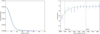 |
Fig. 2. Left panel: beam profile. Right panel: transfer function profile. Measured profiles are in blue, the approximations used for Fig. 6 in green. |
4.2. Model definition
By leaving all the gNFW parameters in Eq. (1) free, we found that parameter c is unconstrained by the data; therefore, we fixed c = 0.014 as in Adam et al. (2015) and let the other parameters free to vary. As priors we took
where P0 is expressed in keV cm−3 and rp in kpc.
We ran 5000 iterations of 14 chains and considered the first 3000 as the burn-in period. We extracted the starting values of the chains from a Gaussian distribution with μ = (0.4, 300, 1.33, 4.13) and σ = 0.1 for all parameters. We considered a sampling step of 2 arcsec and a cluster radial extent of 5 Mpc for the Abel integral computation. The Compton y to Jy beam−1 conversion factor is taken from Adam et al. (2015). We adopt a flat ΛCDM cosmology with H0 = 67.32 km s−1 Mpc−1, ΩM = 0.3158, and ΩΛ = 0.6842 (Planck Collaboration VI 2019).
4.3. Results
Trace plot and joint plus marginal posterior distributions, which are automatically produced by PreProFit, are shown in Fig. 3. The trace plot suggests that the chains adequately explored the parameter space and this regular behaviour is confirmed by the acceptance fraction value equal to 0.43. As expected, b is largely degenerate with rp. Figure 4, which is automatically generated as well, shows the best-fit profile and its 95% CI superimposed on the observed data. We found χ2 = 24.2 for 15 degrees of freedom.
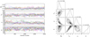 |
Fig. 3. Diagnostic plots automatically produced by PreProFit. Left panel: trace plot. Right panel: joint and marginal posterior distributions. |
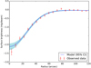 |
Fig. 4. Surface brightness profile (points with 68% error bars) and best fitting profile with 95% CI. This plot is automatically generated by PreProFit. |
Figure 5 compares our pressure profile against corresponding published results from Romero et al. (2018) and Adam et al. (2015) using the same NIKA data, even though they are differently reduced, and therefore have a different transfer function. The former made a non-parametric fit, which requires an unknown and uncertain deprojection correction of the outermost point, not included in the error budget. The latter added Planck and Chandra data and performed a joint fit: we read values without errors from their Fig. 8. There is a good agreement among the three derivations, except at scales corresponding to the instrument radial field of view (around 1 Mpc), where derivations are uncertain, as is clearly documented in the literature (e.g. Sayers et al. 2016; Romero et al. 2019).
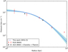 |
Fig. 5. Comparison of CL J1226.9+3332 pressure profiles. Our best fit is plotted in blue (95% CI shaded); the red points are from the non-parametric fit of Romero et al. (2018) on NIKA data (68% error bars); the black diamonds without error bars refer to the fit of Adam et al. (2015) on NIKA, Chandra, and Planck data. |
In Fig. 6, we demonstrate how close or different the results from either measured or approximated instrumental data turn out to be. Differences across surface brightness profiles are comparable to observed errors, indicating that approximated beam and transfer functions might be suitable for feasibility studies, but are unlikely to be useful for science analyses for data of this quality.
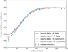 |
Fig. 6. Surface brightness profiles derived for various combinations of beam and transfer function, as specified in the inset, for a single set of pressure profile parameters. Points with 68% error bars show the data. |
5. Conclusion
The amount of data collected through SZ observations has regularly increased in recent years. We have introduced a Python program, PreProFit, that allows users to estimate the pressure profile of galaxy clusters through flexible and efficient modelization. PreProFit is the first publicly available code to perform this kind of analysis and, notably, it is extensively documented; by allowing the analysis of data coming from different sources, it can be useful to a wide community. PreProFit relies on a Bayesian forward-modelling approach.
Users are free to set up PreProFit in accordance with their needs and requirements. Among other things, users can decide how many and which parameters to fit, which (uniform) prior to adopt for the free parameters, and whether to conduct a feasibility study using approximations for the beam and the transfer function. PreProFit returns χ2, model parameters and uncertainties, marginal and joint probability contours, diagnostic plots, and surface brightness radial profiles.
After describing in detail each stage of the data processing pipeline, we presented an application of the program on the high-redshift galaxy cluster CL J1226.9+3332, using SZ observations from the NIKA camera. We outlined the main plots and Bayesian diagnostics produced by PreProFit. We noted that, as is documented in the literature (e.g. Sayers et al. 2016; Romero et al. 2019), it is very difficult to constrain the pressure profile near or beyond the instrument radial field of view.
The release of PreProFit lays the groundwork for an enhanced version of the code that allows us to join the SZ analysis to a three-dimensional (RA, Dec, energy) analysis of X-ray data to perform a powerful joint SZ-plus-X analysis.
New IRAM KIDs Array.
Goddard IRAM Superconducting Millimiter Observatory.
Institut de Radio Astronomie Millimétrique.
Multiplex SQUID TES Array at Ninety GHZ.
Multiwavelength Submillimeter kinetic Inductance Camera.
Atacama Large Millimeter/submillimeter Array.
Atacama Compact Array.
Combined Array for Research in Millimeter-wave Astronomy.
The transfer function (transmission) is often obtained as the square root of the ratio of the one-dimensional power spectra of the observed fake sky and input fake sky (Romero et al. 2017).
Acknowledgments
We thank the referee for the useful comments on the manuscript. F.C. acknowledges financial contribution from the agreement ASI-INAF n.2017-14-H.0 and PRIN MIUR 2015 Cosmology and Fundamental Physics: Illuminating the Dark Universe with Euclid.
References
- Adam, R., Comis, B., Macías-Pérez, J. F., et al. 2015, A&A, 576, A12 [NASA ADS] [CrossRef] [EDP Sciences] [Google Scholar]
- Austermann, J. E., Beall, J. A., Bryan, S. A., et al. 2018, J. Low Temp. Phys., 193, 120 [NASA ADS] [CrossRef] [Google Scholar]
- Banse, K., Crane, P., Grosbol, P., et al. 1983, The Messenger, 31, 26 [NASA ADS] [Google Scholar]
- Birkinshaw, M., & Lancaster, K. 2005, in Background Microwave Radiation and Intracluster Cosmology, eds. F. Melchiorri, & Y. Rephaeli, 127 [Google Scholar]
- Calvo, M., Benoît, A., Catalano, A., et al. 2016, J. Low Temp. Phys., 184, 816 [NASA ADS] [CrossRef] [Google Scholar]
- Comis, B., de Petris, M., Conte, A., Lamagna, L., & de Gregori, S. 2011, MNRAS, 418, 1089 [NASA ADS] [CrossRef] [Google Scholar]
- Czakon, N. G., Sayers, J., Mantz, A., et al. 2015, ApJ, 806, 18 [NASA ADS] [CrossRef] [Google Scholar]
- Dicker, S. R., Ade, P. A. R., Aguirre, J., et al. 2014, J. Low Temp. Phys., 176, 808 [NASA ADS] [CrossRef] [Google Scholar]
- Dicker, S. R., Korngut, P. M., Mason, B. S., et al. 2008, SPIE Conf. Ser., 7020, 702005 [Google Scholar]
- Donahue, M., Voit, G. M., Mahdavi, A., et al. 2014, ApJ, 794, 136 [NASA ADS] [CrossRef] [Google Scholar]
- Ebeling, H., Jones, L. R., Fairley, B. W., et al. 2001, ApJ, 548, L23 [NASA ADS] [CrossRef] [Google Scholar]
- Foreman-Mackey, D., Hogg, D. W., Lang, D., & Goodman, J. 2013, PASP, 125, 306 [CrossRef] [Google Scholar]
- Goodman, J., & Weare, J. 2010, Appl. Math. Comput. Sci., 5, 65 [Google Scholar]
- Jones, E., Oliphant, T., Peterson, P., et al. 2001, SciPy: Open source scientific tools for Python [Online; accessed 2015–04-14] [Google Scholar]
- Korngut, P. M., Dicker, S. R., Reese, E. D., et al. 2011, ApJ, 734, 10 [NASA ADS] [CrossRef] [Google Scholar]
- Maughan, B. J., Jones, L. R., Ebeling, H., & Scharf, C. 2004, MNRAS, 351, 1193 [NASA ADS] [CrossRef] [Google Scholar]
- Maughan, B. J., Jones, C., Jones, L. R., & Van Speybroeck, L. 2007, ApJ, 659, 1125 [NASA ADS] [CrossRef] [Google Scholar]
- Monfardini, A., Swenson, L. J., Bideaud, A., et al. 2010, A&A, 521, A29 [NASA ADS] [CrossRef] [EDP Sciences] [Google Scholar]
- Mroczkowski, T., Bonamente, M., Carlstrom, J. E., et al. 2009, ApJ, 694, 1034 [NASA ADS] [CrossRef] [Google Scholar]
- Nagai, D., Kravtsov, A. V., & Vikhlinin, A. 2007, ApJ, 668, 1 [NASA ADS] [CrossRef] [Google Scholar]
- Planck Collaboration Int. V. 2013, A&A, 550, A131 [NASA ADS] [CrossRef] [EDP Sciences] [Google Scholar]
- Planck Collaboration VI. 2019, A&A, submitted [arXiv:1807.06209] [Google Scholar]
- Romero, C. E., Mason, B. S., Sayers, J., et al. 2015, ApJ, 807, 121 [NASA ADS] [CrossRef] [Google Scholar]
- Romero, C. E., Mason, B. S., Sayers, J., et al. 2017, ApJ, 838, 86 [NASA ADS] [CrossRef] [Google Scholar]
- Romero, C., McWilliam, M., Macías-Pérez, J. F., et al. 2018, A&A, 612, A39 [NASA ADS] [CrossRef] [EDP Sciences] [Google Scholar]
- Romero, C. E., Sievers, J., Ghirardini, V., et al. 2019, ApJ, submitted [arXiv:1908.09200] [Google Scholar]
- Ruppin, F., Adam, R., Comis, B., et al. 2017, A&A, 597, A110 [NASA ADS] [CrossRef] [EDP Sciences] [Google Scholar]
- Ruppin, F., Sembolini, F., De Petris, M., et al. 2019, A&A, 631, A21 [NASA ADS] [CrossRef] [EDP Sciences] [Google Scholar]
- Sayers, J., Czakon, N. G., Day, P. K., et al. 2010, SPIE Conf. Ser., 7741, 77410W [Google Scholar]
- Sayers, J., Czakon, N. G., Mantz, A., et al. 2013, ApJ, 768, 177 [NASA ADS] [CrossRef] [Google Scholar]
- Sayers, J., Golwala, S. R., Mantz, A. B., et al. 2016, ApJ, 832, 26 [NASA ADS] [CrossRef] [Google Scholar]
- Staguhn, J., Allen, C., Benford, D., et al. 2008, J. Low Temp. Phys., 151, 709 [NASA ADS] [CrossRef] [Google Scholar]
- Sunyaev, R. A., & Zeldovich, Y. B. 1970, Ap&SS, 7, 3 [NASA ADS] [Google Scholar]
- Sunyaev, R. A., & Zeldovich, Y. B. 1972, Comments Astrophys. Space Phys., 4, 173 [NASA ADS] [EDP Sciences] [Google Scholar]
- Woody, D. P., Beasley, A. J., Bolatto, A. D., et al. 2004, in SPIE Conf. Ser., eds. C. M. Bradford, P. A. R. Ade, J. E. Aguirre, et al., 5498, 30 [NASA ADS] [Google Scholar]
All Figures
|
Fig. 1. Block diagram showing the program flow. |
| In the text | |
|
Fig. 2. Left panel: beam profile. Right panel: transfer function profile. Measured profiles are in blue, the approximations used for Fig. 6 in green. |
| In the text | |
|
Fig. 3. Diagnostic plots automatically produced by PreProFit. Left panel: trace plot. Right panel: joint and marginal posterior distributions. |
| In the text | |
|
Fig. 4. Surface brightness profile (points with 68% error bars) and best fitting profile with 95% CI. This plot is automatically generated by PreProFit. |
| In the text | |
|
Fig. 5. Comparison of CL J1226.9+3332 pressure profiles. Our best fit is plotted in blue (95% CI shaded); the red points are from the non-parametric fit of Romero et al. (2018) on NIKA data (68% error bars); the black diamonds without error bars refer to the fit of Adam et al. (2015) on NIKA, Chandra, and Planck data. |
| In the text | |
|
Fig. 6. Surface brightness profiles derived for various combinations of beam and transfer function, as specified in the inset, for a single set of pressure profile parameters. Points with 68% error bars show the data. |
| In the text | |
Current usage metrics show cumulative count of Article Views (full-text article views including HTML views, PDF and ePub downloads, according to the available data) and Abstracts Views on Vision4Press platform.
Data correspond to usage on the plateform after 2015. The current usage metrics is available 48-96 hours after online publication and is updated daily on week days.
Initial download of the metrics may take a while.