| Issue |
A&A
Volume 632, December 2019
|
|
|---|---|---|
| Article Number | A125 | |
| Number of page(s) | 17 | |
| Section | Numerical methods and codes | |
| DOI | https://doi.org/10.1051/0004-6361/201936404 | |
| Published online | 16 December 2019 | |
Synthesising the intrinsic FRB population using frbpoppy
1
ASTRON – the Netherlands Institute for Radio Astronomy, Oude Hoogeveensedijk 4, 7991 PD Dwingeloo, The Netherlands
e-mail: This email address is being protected from spambots. You need JavaScript enabled to view it.
2
Anton Pannekoek Institute for Astronomy, University of Amsterdam, Science Park 904, 1098 XH Amsterdam, The Netherlands
Received:
30
July
2019
Accepted:
16
October
2019
Abstract
Context. Fast radio bursts (FRBs) are radio transients of an unknown origin whose nature we wish to determine. The number of detected FRBs is large enough for a statistical approach to parts of this challenge to be feasible.
Aims. Our goal is to determine the current best-fit FRB population model. Our secondary aim is to provide an easy-to-use tool for simulating and understanding FRB detections. This tool can compare surveys, or provide information about the intrinsic FRB population.
Methods. To understand the crucial link between detected FRBs and the underlying FRB source classes, we performed an FRB population synthesis to determine how the underlying population behaves. The Python package we developed for this synthesis, frbpoppy, is open source and freely available. frbpoppy simulates intrinsic FRB populations and the surveys that find them with the aim to produce virtual observed populations. These populations can then be compared with real data, which allows constraints to be placed on the underlying physics and selection effects.
Results. We are able to replicate real Parkes and ASKAP FRB surveys in terms of detection rates and observed distributions. We also show the effect of beam patterns on the observed dispersion measure distributions. We compare four types of source models. The “complex” model, featuring a range of luminosities, pulse widths, and spectral indices, reproduces current detections best.
Conclusions. Using frbpoppy, an open-source FRB population synthesis package, we explain current FRB detections and offer a first glimpse of what the true population must be.
Key words: radio continuum: general / methods: statistical
© ESO 2019
1. Introduction
Fast radio bursts (FRBs) are bright, brief, and baffling radio transients. Since their discovery at the Parkes telescope (Lorimer et al. 2007; Thornton et al. 2013), an array of other surveys have also detected FRBs (e.g. Spitler et al. 2014; Masui et al. 2015; Farah et al. 2018; Bannister et al. 2017; Petroff et al. 2019). The large majority of these appear as one-off bursts, despite extensive dedicated programs of several hundreds of hours (e.g. Petroff et al. 2015; Shannon et al. 2018). Some FRB sources have, however, been found to repeat (Spitler et al. 2016; The CHIME/FRB Collaboration 2019). The observed dispersion measure (DM) excess beyond the Galactic contribution places all FRBs at extragalactic distances, which indeed is one of their defining features. Localised FRBs confirm this theory, showing them to originate from host galaxies other than our own at gigaparsec distances (Tendulkar et al. 2017; Bannister et al. 2019; Ravi et al. 2019a). These FRBs allow us to start mapping out the relationship between the distance and the DM contribution from traversing the intergalactic medium. As a result, FRBs have been hailed as possible cosmological probes that can in principle provide information about the intergalactic medium (Macquart & Koay 2013), baryonic content (McQuinn 2014) or about the large-scale structure in the Universe (Masui & Sigurdson 2015). To infer the characteristics of our Universe, however, we need in practice to understand the dispersion measure contributions of the source themselves, for instance: we need to known the volumetric rate and properties of the intrinsic population.
The first ten years of research in this field yielded only a handful of FRB detections1. Without stringent observational constraints, no consensus on the origin of FRBs could emerge. A large number of theories on the origin of FRBs have therefore been presented (see Platts et al. 2019) with suggestions ranging from young pulsars (e.g. Connor et al. 2016a) to active galactic nuclei (AGNs; e.g. Vieyro et al. 2017). The advent of all-sky surveys such as CHIME (The CHIME/FRB Collaboration 2018) and of surveys with a high spatial and fluence precision such as ASKAP (Shannon et al. 2018) and Apertif (Maan & van Leeuwen 2017) will drastically change this field. Their high detection rates and improved localisations will enable mapping the observable FRB population much more thoroughly. This presents the next challenge: determining the nature of FRBs from this observed population.
With the expected high FRB detection rates, it is essential that we understand what the detected FRBs represent. Directly taking the observed properties of an FRB population as representative of the underlying source class will often be incorrect. A variety of selection effects, whether due to telescope sensitivity, wavelength range, search parameters, or even time resolution, will prohibit a direct match. These seemingly obvious selection effects tells us that similar selection effects must, potentially more subtly, be at play for many other FRB traits. It is therefore essential that the mix of intrinsic FRB properties, propagation effects, and selection effects are understood.
Population synthesis is a method through which the details of an intrinsic source population can be probed. Population synthesis provides statistical insights into the parent population and is helpful when the number of observed sources is small and where observational biases cannot easily be corrected for analytically. This method is especially powerful when the underlying class is much larger and potentially more diverse than the population that is observed. In practice, population synthesis thus consists of three components: modelling a population, applying selection effects by modelling a survey, and comparing the simulated results to real detections. This process is then repeated by adapting the modelled population or modelled survey until the results are in good agreement with each other. Each iteration in synthesising populations or modelling selection effects allows an increasingly accurate model of the underlying population to be built. In this way, population synthesis not only provides insight into an intrinsic source population, but also into the often complex convolution of selection effects.
This method has previously been successfully applied to a variety of astronomical phenomena, such as pulsars (Taylor & Manchester 1977), gamma ray bursts (Ghirlanda et al. 2013), and stellar evolution (Izzard & Halabi 2018). Like the FRBs under consideration in this work, pulsars are time-domain sources, and many of the selection effects are identical. Gunn & Ostriker (1970) started with fewer pulsars, 41, than there are FRBs now, and because period derivatives had not yet been measured for most, very little was known about these pulsars. When new surveys had increased the detected sample tenfold, Lyne et al. (1985) were able to estimate birth rates, and Bhattacharya et al. (1992) determined the longevity of the magnetic field. Using the modern sample of over 2000 pulsars, statistical studies of radio-beaming fractions (van Leeuwen & Verbunt 2004), birth locations (Faucher-Giguère & Kaspi 2006), and radio luminosities (Szary et al. 2014), for instance, have improved our understanding of the pulsar population. These parent populations can be used to optimise the strategies for pulsar surveys such as using LOFAR (van Leeuwen & Stappers 2010) and the Square Kilometre Array (SKA; Smits et al. 2009), and to predict the outcomes to within a factor of a few (cf. Sanidas et al. 2019).
Unfortunately, next to none of the synthesis codes that produced the work mentioned above were made public. An argument over two versus one pulsar birth populations (Narayan & Ostriker 1990 versus Bhattacharya et al. 1992) was therefore at least partly fueled by incomplete understanding of the used codes, which were both proprietary and closed. The synthesis work by Smits et al. (2009) and Lorimer et al. (2006), however, was reproducible because the authors based their research on PSRPOP (Lorimer 2011) and PsrPopPy (Bates et al. 2014, 2015).
Prior efforts at FRB population synthesis have mostly been directed towards dedicated surveys. Several primarily searched for FRB volumetric densities (e.g. Caleb et al. 2016a; Fialkov et al. 2018; Niino 2018; Bhattacharya et al. 2019), and others focused on the origin of the excess dispersion measure (Walker et al. 2018), on spectral indices (Chawla et al. 2017), on brightness distributions (Oppermann et al. 2016; Vedantham et al. 2016; Macquart & Ekers 2018a,b), and on repeat fractions (Caleb et al. 2019). Despite the large variety of FRB population synthesis models, the underlying code is not always provided or easily adaptable.
It is important that FRB detections are reported with a full understanding of underlying selection effects, and by extension, their relation to the intrinsic FRB population. An open platform for FRB population synthesis can facilitate this, which is why we have developed frbpoppy (Fast Radio Burst POPulation synthesis in PYthon). This open-source software package aims to be modular and easy to use, allowing survey teams to understand implications of new detections. frbpoppy can help in the study of FRB population features and in predicting future results, just as pulsar population synthesis did for the pulsar community.
In this paper we aim to determine what the real FRB parent population must look like, and we present the first version of frbpoppy (v1.0.0), which is accessible on Github2. We start the paper by describing the simulation process in frbpoppy, before demonstrating some applications of the code in the second half of the paper. Accordingly, Sect. 2 describes how an intrinsic FRB population is simulated, Sect. 3 describes how a survey is simulated, Sect. 4 describes how real detections are used, and Sect. 5 details how we compare simulated and real FRB populations. In Sect. 6 we describe results, and in Sect. 7 we discuss that a simple, local population of standard candles cannot describe current observations. A cosmological population, with a specific distribution of pulse widths, spectral indexes, and luminosities, is required to reproduce the observed FRB sky. The paper concludes in Sect. 8, and additional information is provided in Appendix A.
2. Generating an FRB population
The main goal in population synthesis is to infer the properties of the real underlying parent population through a simulated population. Following conventions in pulsar population synthesis (e.g. Bhattacharya et al. 1992), we aim to keep a clear distinction between these real and simulated FRB populations. Both real and simulated experiments deal with two sets of distributions: The intrinsic physical properties of the populations, including their luminosity function and redshift distribution, and their observed properties, for example the brightness and DM distributions. We use the terms “underlying”, “parent”, and “progenitor” interchangeably with the former, and we use the phrase “surveyed” or “detected” synonymously with “observed”. We refer to FRBs that are generated and observed in the frbpoppy framework as simulated and to actual FRBs as real.
Following conventions in pulsar population synthesis (e.g. Bhattacharya et al. 1992), we aim to keep a clear distinction between these real and simulated FRB populations. Both real and simulated experiments deal with two sets of distributions: The population’s intrinsic physical properties, including their luminosity function and redshift distribution, as well as their observed properties, for example the brightness and DM distributions. We use the terms “underlying”, “parent”, and “progenitor” interchangeably with the former, and we use the phrase “surveyed” or “detected” synonymously with “observed”. We refer to FRBs generated/observed in the frbpoppy framework as simulated and actual FRBs as real.
Our method consists of three parts: modelling an intrinsic population, applying selection effects, and comparing the simulated population to real detections. Out of these three components, the modelling of an intrinsic FRB population allows the underlying physics to be probed. This we do by first formulating a hypothesis on what the parent population is and how it behaves. We subsequently translate this into the parameters available in frbpoppy, listed in Table 1. These can be adjusted to simulate for example different source-class densities and emission characteristics, or propagation effects. By doing this for various models, running the population synthesis separately on each, and comparing the outcome (cf. Sect. 7), we can learn which underlying population best describes the observed FRB sky. In this paper we compare four models. The adopted values for each are listed in Table 1. Using these, we aim to answer questions such as whether the host dispersion measure has a measurable influence on the population that our telescopes detect. We also study whether a model employing standard candles can reproduce the observed fluence distributions. The subsequent sections describe each of the model aspects.
Overview of the parameters that are required to generate an initial cosmic FRB population.
2.1. Number density
We first aim to determine the volumetric rate of FRB progenitors that is needed to reproduce the observed sample. To establish the underlying number density of FRB sources, we modelled a number of population characteristics. In the work presented here, we limit ourselves to one-off FRBs and leave the treatment of repeating FRBs to the near future. All FRB setups generate sources that are isotropically distributed on the sky; with individual distances being set by the following source number density models:
Constant. FRBs have a constant number density per comoving volume element such that
 (1)
(1)
with ρFRB(z) the constant number density of FRBs such that there is no redshift dependence. Given ρFRB(z) = dN/dVco with the differential number of FRBs dN in a comoving volume element dVco, dN = ρFRB(z) ⋅ dVco = C ⋅ dVco and so dN ∝ dVco. We can therefore simulate a constant number density distribution by uniformly sampling a comoving volume Vco space. In frbpoppy we convert a given maximum redshift to the corresponding maximum comoving volume such that this space can be sampled using
 (2)
(2)
with the comoving volume of an FRB Vco, FRB, the maximum comoving volume Vco, max, and a random number from a uniform distribution with U ∈ [0, 1]. Conversions to luminosity distance and redshift, for instance, are based on Wright (2006) using cosmological parameters from Planck Collaboration XIII (2016). These parameters are listed in Table 1.
Star formation rate (SFR). The FRB number density is proportional to the comoving SFR. We followed Madau & Dickinson (2014), who derived that the SFR follows
![Mathematical equation: $$ \begin{aligned} \rho _{\rm FRB}(z) \propto \frac{(1+z)^{2.7}}{1+[(1+z)/2.9]^{5.6}}, \end{aligned} $$](/articles/aa/full_html/2019/12/aa36404-19/aa36404-19-eq3.gif) (3)
(3)
with ρFRB(z) the comoving number density of FRBs at a given redshift z. We sample this distribution by numerical constructing a cumulative distribution function (CDF) of Eq. (3) over redshift. Uniformly sampling this CDF provides the corresponding redshift distribution, which can then be converted into any other required cosmological distances.
Stellar mass density (SMD). The FRBs follow the relationship between redshift and cosmic stellar mass density as given by Madau & Dickinson (2014), using
![Mathematical equation: $$ \begin{aligned} \rho _{\rm FRB}(z) \propto \int _{z}^\infty \frac{(1+z^{\prime })^{1.7}}{1+[(1+z^{\prime })/2.9]^{5.6}} \frac{\mathrm{d}z^{\prime }}{H(z^{\prime })}, \end{aligned} $$](/articles/aa/full_html/2019/12/aa36404-19/aa36404-19-eq4.gif) (4)
(4)
with ρFRB(z) the number density at redshift z and H(z′) the Hubble parameter in a flat cosmology such that the spatial curvature density parameter Ωk is zero. H(z′) can then be further defined as
 (5)
(5)
with the Hubble parameter H0, the matter density parameter Ωm, and the dark energy density parameter Ωλ (Madau & Dickinson 2014). We simulated the SMD in a manner similar to the SFR: we first constructed a CDF over redshift for Eq. (4), which we then uniformly sampled to obtain a redshift distribution.
Power law. While a constant number density per comoving volume may work in many cases, the ability to vary this density can be helpful. For example, modelling a relative overabundance of local FRBs can prove interesting. To this end, we also modelled various density-distance relations with
 (6)
(6)
following Eq. (2) in setting Vco, but instead scaling the uniform sampling U(0, 1) by β. This exponent β allows for instance for relatively more local sources and less distant sources to be generated. When it is combined with the luminosity function and the instrument response, this number density relation to distance (and hence, fluence) will determine the observed brightness distribution of FRBs.
Rather than using β as input, out of convenience a different expression can be used,
 (7)
(7)
with β the power as given in Eq. (6) and αin an input parameter. In a Euclidean universe, the total number of sources N out to a radius R scales as N(< R)∝R3. Combined with the flux S scaling as S ∝ R−2, we can derive for standard candles N(> S)∝S−3/2. This exponent of the log N–log S relation can also be expressed as α, so that for a Euclidean universe, α is expected to equal −3/2. However, when a power-law relation is chosen in frbpoppy, these relationships change. Instead, as a result of the change in sampling the comoving volume, N(< R)β ∝ R3, or N(< R)∝R3/β, leading to N(> S)∝S−3/(2β). Given Eq. (7), this is equivalent to saying N(> S)∝Sαin. Equation (7) therefore allows αin to have a value such that if a Euclidean population was observed with a perfect survey, αin would equal the observed slope α of the log N–log S relation. In different words, within the FRB detection completeness in the very nearby universe, α = αin. Extending this to cosmological distances says that surveying any FRB population with a given αin would result in an observed log N–log S slope asymptoting towards αin in the limit of the local Universe. An extensive discussion of this topic can be found in Macquart & Ekers (2018a).
Figure 1 shows five populations following the models described above, with the constant number density population showing clear cosmological effects with increasing redshift. This behaviour, in which the number density flattens out at higher redshifts, is as expected because volume runs out towards larger cosmological distances. The corresponding comoving volume V(z) at redshift z matches the volumes calculated following Hogg (1999).
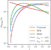 |
Fig. 1. Comoving number density (ρ(z)≡dN/dz) as a function of redshift from a simulated distribution of 106 FRBs. The FRBs either follow a constant number density per comoving volume element (Wright 2006), the SFR (Madau & Dickinson 2014), the SMD (Madau & Dickinson 2014), or a power law in the comoving volume space with index αin = −0.5 or αin = −2.0 (see Sect. 2.1). Note that dnFRB refers to the intrinsic number of FRBs and not to an observed number because that would be affected by a factor of (1 + z)−1 as well as the luminosity function, spectral index, etc. |
2.2. Dispersion measure
The dispersion measure quantifies the relative arrival time of an FRB with respect to its highest frequency and is defined such that
 (8)
(8)
with the rest frame dispersion measure DM, distance d, electron number density ne, and differential step dl (Lorimer & Kramer 2012). This measure represents the column density of free electrons along the line of sight, but is mute on the location of these electrons. Most cosmology tests with FRBs require an understanding of the various contributors to the total observed dispersion measure. We thus modelled the total dispersion measure as the addition of several components, to aid in assigning different certainties and models to each,
 (9)
(9)
with the total dispersion measure DMtot, the dispersion measure contribution by the host galaxy DMhost adapted by the redshift z (Tendulkar et al. 2017), the contribution from the intergalactic medium DMIGM, and finally, the Milky Way component DMMW.
2.2.1. Dispersion measure – host
Lacking strong constraints on the host galaxy dispersion measure, we followed Thornton et al. (2013) and adopted a value of 100 pc cm−3, and adding a Gaussian spread to this value while ensuring DMIGM > 0 pc cm−3. Using such a distribution, we can replicate observations that appear to indicate a varying dispersion measure contribution from the host galaxy and/or source (e.g. Michilli et al. 2018). A variety of models are available in frbpoppy, allowing the DMIGM to more accurately represent future observations.
2.2.2. Dispersion measure – IGM
Modelling the free electron density in the intergalactic medium is a challenging task, whether in distinguishing contributions from the Milky Way or host, or even in obtaining observations capable of probing this intervening matter. While often an approximation of DMIGM ≈ 1200z is used for the contribution of the intergalactic medium to the total dispersion measure (Ioka 2003; Inoue 2004), recent research seems to be tending towards values in the range of 800−1000 pc cm3 (e.g. Zhang 2018; Keane 2018; Pol et al. 2019), or non-linear relationships such as given in Batten (2019). We here drew the value of DMIGM for an FRB at redshift z from a Gaussian distribution 𝒩(1000z, 200z), with 𝒩(μ, σ) denoting the values for the mean μ and a standard deviation σ. In this way, a scatter around a linear relationship between DMIGM and z is introduced. This method can be updated as new information becomes available (e.g. Bannister et al. 2019; Ravi et al. 2019b).
2.2.3. Dispersion measure – Milky Way
With over 50 years of pulsar observations (Hewish et al. 1968), the Galactic dispersion measure has better constraints than that of the intergalactic medium. For the current work, we followed Cordes & Lazio (2002). Developed as a tool for estimating pulsar dispersion measures in the Milky Way, it is a familiar model to those working in the field, even though some of its distance measurements are older than those in Yao et al. (2017), for example. We used the dispersion measure values taken in each direction queried at a distance of 100 kpc to retrieve the maximum Galactic dispersion measure. This distance also surpasses the maximum radial extent of the thick disc of 20 kpc in every direction (Cordes & Lazio 2003). Other models can of course be added to frbpoppy by those interested.
2.3. Luminosity
Determining the correct intrinsic FRB luminosity distribution may tell us how FRBs radiate. A number of radiation models have been suggested (e.g. Katz 2014; Romero et al. 2016; Lu & Kumar 2018; Metzger et al. 2019; Beloborodov 2019). Without observational constraints on the intrinsic emission mechanism of FRBs, sources in frbpoppy are assumed to be radiating isotropically. Luminosities are generated following a power-law distribution, with options to set the index (Lbol, index), and the minimum and maximum value (Lbol, range). While for example Caleb et al. (2016a) also adopted power-law functions, Luo et al. (2018) and Fialkov et al. (2018) recently indicated that a Schechter luminosity function might provide a more accurate description. While in this initial version of frbpoppy we only include a power-law model, other distributions such as a Schechter luminosity function or a broken power law could be implemented in future iterations.
2.4. Spectral index
To further understand the FRB emission process, we aim to learn whether they emit over a wide spectrum, and at which frequencies they are brightest. In frbpoppy, as in psrpoppy, we thus allow the intrinsic spectral indices for individual FRBs to be drawn from a Gaussian distribution for which the mean and standard deviation can be set. We define the spectral index γ such that
 (10)
(10)
with the energy Eν at the rest-frame frequency ν′ (Lorimer et al. 2013). Because the intrinsic spectral index of the FRB population has proven difficult to determine (e.g. Spitler et al. 2014; Scholz et al. 2016), we draw γ from a Gaussian distribution centred around −1.4 with a standard deviation of 1, as in Bates et al. (2013). This replicates observations of the Galactic pulsar population. Macquart et al. (2019) recently favoured similar values for the FRB population.
2.5. Pulse width
Determining the intrinsic FRB pulse widths can elucidate some very specific traits of the source environment, such the size of the emitting region, or the beaming fraction for a rotating source. Because the observed FRB pulse width detections cluster around millisecond timescales, we used as input one of two models that we call “uniform” or “lognormal”:
Uniform. The pulse width values were chosen randomly between a given lower and higher millisecond timescale.
Lognormal. In order to replicate the distribution of pulse widths observed in pulsars, or indeed repeater pulses, we drew pulse widths from a log-normal distribution. The probability density function that a variable x is considered to have a log-normal distribution can be expressed as
 (11)
(11)
for the variable x, standard deviation σ, and mean μ (Johnson 1994). frbpoppy provides options to adapt the mean and standard deviation of this distribution, which can be adjusted to replicate broad or narrow pulse widths.
2.6. Number of sources
Internally, the simulated FRB population is formed by a certain total number of sources (ngen). The value of this parameter will depend on the resolution sought in the resulting population, while taking a wide range of selection effects into account. Based on results from the high-latitude HTRU survey, Thornton et al. (2013) measured an FRB rate of  sky−1 day−1 above a 3 Jy ms threshold. Subsequent detections updated the rate to
  sky−1 day−1 (Champion et al. 2016), and taking completeness into account, Keane & Petroff (2015) measured a rate of 2500 sky−1 day−1 above a 1.4 GHz fluence of 2 Jy ms. Therefore, unless the aim is to use a “perfect” survey, that is, a survey in which all FRBs are detected, cosmic FRB populations should be generated with > 104 FRBs to ensure sufficient simulated detections. Population and survey parameter choices have a strong influence on this number, and this value is therefore given solely as a very rough indication.
2.7. Number of days
Setting the number of days over which a population of FRBs is emitted (ndays) provides a way to set a volumetric rate. Within this paper, all detection rates are scaled relative to each other, and accordingly, the number of days is set to one. This parameter can be used coupled with the number of survey days, however, to obtain a simulated absolute detection rate. Matching this to a real detection rate allows probing the volumetric rate of FRBs.
3. Observing an FRB population
The observed FRB population will always differ from the intrinsic population: the former involves a number of selection effects that are layered on top of the intrinsic FRB population (Connor 2019). The following section describes how we constructed virtual surveys, each with different celestial selection effects, for instance, and hardware constraints.
3.1. Surveys
The telescope with which a survey is conducted can cause a large variety of selection effects. For example, surveys are biased against detecting both narrow pulses and highly dispersed pulses because the finite time and frequency resolution of the instruments results in deleterious smearing effects (Connor 2019). The strength of these hardware selection effects can vary per survey, however. These very same selection effects have been long known to be highly important for pulsar surveys (e.g. Taylor & Manchester 1977).
In Table 2 we present an overview of the survey parameters adopted within frbpoppy. With these parameters, a survey model can be constructed. From these parameters we infer the resultant selection effects to model the expected survey rates and parameter distributions. While the values in Table 2 are sufficient to reproduce the results found in the current work, additional surveys are already included in frbpoppy, and new surveys are easy to implement. CHIME, for instance, already detects FRBs at a very high rate, but it is not included in this work because we are not yet sufficiently confident in modelling its system parameters. It is also the only survey with detections below 700 MHz. Still, an early version of this survey model is included in frbpoppy, and subsequent research will cover CHIME detections.
Overview of survey parameters used in this paper.
3.2. Pulse width
A variety of effects modify the FRB pulses as they travel through space, and are detected on Earth. The first effect is purely cosmological. Depending on the method used to populate the simulated FRB event space, a comoving distance might need to be calculated from a redshift distribution, or the inverse. With both of these taking place over large distances, cosmology must be taken into account when parameter values upon arrival at Earth are calculated, rather than simply taking the initial value. The pulse width of an FRB arriving at Earth is then
 (12)
(12)
where the intrinsic pulse width wint at redshift z has been dilated to the pulse width as it arrives at Earth, warr.
The second effect, in principle, is the increase of the observed pulse width due to multi-path scattering. In frbpoppy the parameter tscat allows scattering timescales to be included in calculating the effective pulse width. The adaptation of Bhat et al. (2004) to FRBs from Lorimer et al. (2013) is included in frbpoppy, being
 (13)
(13)
with the scattering timescale tscat, the total dispersion measure DMtot, and the central survey frequency in GHz νc. A Gaussian scatter is subsequently applied such that
 (14)
(14)
with the scattering timescale tscat and a Gaussian function 𝒩(μ, σ) with the mean μ and standard deviation σ. The current FRB population appears to be underscattered relative to Galactic pulsars (see e.g. Ravi 2019). Many FRB profiles show scattering, but no consistent scattering relation has yet been established and a larger future population may be needed. Because our understanding regarding the scattering properties of FRBs is incomplete (see e.g. Cordes & Wasserman 2016; Xu & Zhang 2016), we set the scattering timescale as a default to zero.
Thirdly, we take into account the effects of intra-channel dispersion smearing tDM, and the sampling time tsamp. Starting with the dispersion smearing, tDM can be calculated following
 (15)
(15)
with the dispersion smearing tDM in ms, the lower and upper frequency of a survey channel ν1 and ν2, respectively, and the central frequency thereof νc, all in MHz (Cordes & McLaughlin 2003), and the total dispersion measure DMtot as given in Eq. (9).
The final term is the sampling timescale tsamp. This is provided as input per survey and can be found in Table 2.
Together these terms contribute to the observed pulse, with weff added as
 (16)
(16)
and this pulse width is used in determining whether the FRB is detected (Lorimer & Kramer 2012).
3.3. Detection
The brightness detection threshold of an FRB can be determined by the radiometer equation for a single pulse,
 (17)
(17)
with the peak flux density  , the gain G, the degradation factor β, the total system temperature Tsys, the number of polarisations npol, the boundary frequencies of a survey ν1, 2, and the pulse width at Earth warr (Lorimer & Kramer 2012; Connor 2019). As the system temperature
 (18)
(18)
with the receiver temperature Trec and sky temperature Tsky (Lorimer & Kramer 2012), Trec joins G, β, npol and ν1, 2 as survey dependent parameters, and can be found in Table 2. We take Tsky to be dominated by synchrotron radiation and scale it as
 (19)
(19)
with the directional dependent values from the 408 MHz sky survey T408 MHz and the central frequency νc (Remazeilles et al. 2015). Returning to Eq. (17), and taking cosmology into account,  can be calculated with
 (20)
(20)
with the luminosity Lbol, the redshift z, the comoving distance D(z), and the spectral index γ (Lorimer et al. 2013; Connor 2019). The luminosity refers to an isotropic equivalent bolometric luminosity in the radio, where the frequency range is defined by νlow, high. This is because we do not include beaming effects, and we do not attempt to model emission outside of νlow and νhigh. We set the boundary emission frequencies of an FRB source νlow, high, to 10 MHz and 10 GHz as a default. The pulse width at Earth warr and effective pulse width weff (Lorimer et al. 2013; Connor 2019) are used to take into account the degradation of the peak flux due to pulse broadening; this in effect raises the detection threshold.
The equations as given above allow a brightness threshold for an FRB detection to be set, but do not automatically equate to a detection. To this end, the signal-to-noise ratio (S/N) of each FRB must first be convolved with a beam pattern.
3.4. Beam patterns
A number of modelled beam patterns are available in frbpoppy. Given the scaled angular distance on the sky from the beam centre r ∈ [0, 1], the following beam models describe the relative sensitivity pattern I(r). The link between beam patterns and observing frequency is modelled in frbpoppy via the field-of-view parameter as given in Table 2, which is presumed to be valid for the central frequency of a survey.
Perfect. A perfect intensity profile, that is, no beam pattern, for testing, and for comparing realistic beam patterns against,
 (21)
(21)
Airy. The beam pattern of a single-dish single-pixel radio telescope can be best described with an Airy disc, for which a simple representation can be made with
 (22)
(22)
Derivations for the equations of the scaling factor k and radial offset N(r) can be found in Appendix A. Both provide scaling factors for the Airy disc.
Gaussian. An additional option is to model the intensity profile as a Gaussian beam,
 (23)
(23)
Here the derivation of the scaling factor M can also be found in Appendix A, relating to the maximum offset. r remains a normalised radial offset from the beam centre to the maximum available offset, being drawn from a uniform distribution such that r ∈ [0, 1].
In Fig. 2 we show examples of these beam patterns, including several side-lobe options for an Airy disc. In the latter cases a side lobe of 0.5 can be chosen to cut the intensity profile at the full width at half-maximum (FWHM). The choice of side lobe sets the maximum radius at which an FRB can still be detected. The difference in sky area covered by an Airy disc without side lobes and an Airy disc with eight side lobes is accounted for within frbpoppy by recalculating the associated beam size.
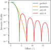 |
Fig. 2. Intensity profile of various beam patterns as function of the radial offset from the centre. The relative scaling on the vertical axis is linked to selected survey’s beam size at FWHM, as calculated from beamsizes seen in Table 2. Up to eight sidelobes can be included in frbpoppy surveys, but the option to simulate a beam out to the FWHM is also possible (as illustrated by the “perfect” beam pattern). |
Parkes. When the beam pattern described in Ravi et al. (2016) is used with an applied scaling between 0 and 1, an FRB can be randomly dropped in the calculated beam pattern, allowing for a more realistic intensity profile model when attempting to reproduce Parkes detections. This beam pattern uses the “MB21” setup, which combines 13 beams spanning 3 × 3° on the sky, and is calculated at 1357 MHz. This is close to the central frequency that is adopted for Parkes in this survey.
Apertif. In a similar fashion as for the Parkes beam model, we can use the intensity profile developed for Apertif (Hess, priv. comm.; Adams & van Leeuwen 2019).
In Fig. 3 we show the distribution of intensity profiles for the Parkes and Apertif beams. Shaded regions depict the range of intensities per radius, and the darker lines indicate the average intensity profile.
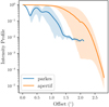 |
Fig. 3. Shaded regions: possible beam intensities of respectively the Parkes Multibeam and Apertif Phased Array Feed (PAF) as a function of radial offset from the centre of the beam (Ravi et al. 2016; Hess, priv. comm.). Solid lines: average intensity profile per survey. |
3.5. Rates
We first determine the registered FRB detections by the S/N limit of a survey (see Table 2). The rate at which FRBs are detected from a given redshift is additionally affected by cosmological time dilation, however. To account for this effect, frbpoppy dilutes the rate of detection by only recording a subset of events from redshift z, with this fraction being equal to to 1/(1 + z). This is done by drawing a random number r ∈ [0, 1] and testing for r ≤ (1 + z)−1. If an FRB satisfies this requirement, it is registered as detected. If it does not, it is registered as too late for detection. This mimics the finite observing window of a real survey.
While frbpoppy uses all detected FRBs (ndet) in simulating observed distributions, for example, it would not be realistic to assume that all generated FRBs happen to land within the beam of the telescope. In order to obtain a realistic detection rate of FRBs rdet, ndet must be scaled by total survey area. This can be scaled from ndet with
 (24)
(24)
with the detection rate rdet, the number of detected FRBs ndet, the number of surveying days ndays, the FoV Abeam, and the size of the survey area Asurvey. Here the number of surveying days ndays has been introduced to be able to discuss the detection rate of a single survey. For a comparison of the detection rates of multiple surveys, this term could removed by normalising the detection rates to that of a single survey. As
 (25)
(25)
in the limit of large n and with nsurvey area all FRBs within the survey area, whether they are detected or not. With
 (26)
(26)
rdet can be calculated as
 (27)
(27)
with the detection rate rdet, the number of detected FRBs ndet, the number of surveying days ndays, the number of simulated FRBs ntot, the number of FRBs falling within the survey area nsurvey area, the FoV Abeam, and the size of the survey area Asurvey.
We note, however, that this equation only holds for a population of one-off FRB events. While there now are two known repeating FRBs (Spitler et al. 2016; The CHIME/FRB Collaboration 2019), the majority of the FRBs in the total population have only been seen once. For instance Ravi (2019) recently seemed to favour the idea that most observed FRBs originate from repeaters. Given the limited understanding of the repeating FRBs found so far, we chose to model FRBs in frbpoppy as single one-off events in this paper, and we choose to focus on repeaters in future work.
3.6. Running frbpoppy
In a setup as described in the sections above, frbpoppy is able to construct a cosmic population with the population parameters given in Table 1. Subsequently, a survey can be modelled using the survey parameters in Table 2. Convolving these two allows a survey population to be simulated. A minimum working example is given below, showing how frbpoppy can be used:
While this shows a basic setup, a wide range of parameters can be given as arguments to these classes, providing the option for a user to tweak populations to their preference. The first run of frbpoppy for a population of this size will typical take < 2 h on a four-core computer, and will create databases for cosmological and dispersion measure distributions. Subsequent runs will take on the order of seconds. Increasing the population size to 108 FRBs on a single core increases the run time to just over 3 h, of which most time is spent on SQL queries to the generated databases.
4. Forming a real FRB population
Real observations are needed to compare our simulations to reality. This section describes the process in which real data were gathered for use within frbpoppy, from FRB parameters to detection rates.
4.1. FRB parameters
To verify simulated FRB distributions, frbpoppy needs real FRB detection survey data. To this end, we used FRBCAT, the online catalogue of FRBs3 (Petroff et al. 2016). Some simple cleaning and conversion algorithms were applied to the database before use. To obtain a single range of parameters per FRB, we filtered the FRBCAT sample by selecting the measurement with the most parameters. By default, repeat pulses were also filtered out to reduce the saturation of distributions by a single FRB source. We subsequently attempted to match all FRBs with an associated survey using a user-predefined list. frbpoppy updates its database monthly if online, and otherwise uses the most recent database. In this paper, all results were run using FRBCAT as available on 23 September 2019. Next to the entire real FRB population, frbpoppy provides the option to select FRBs from a single survey or telescope. An interactive plotting window can compare the chosen populations.
4.2. FRB detection rates
Beyond the parameters of individual FRBs, described above, the rate of detection is important to constrain the intrinsic FRB population. Survey detection rates are not always published, often because of the difficulties in determining the total observing time.
For the surveys that did publish rates, we converted the published rates into rates per survey expressed as the number of FRBs detected per day of observing time. In this paper we adopted
Rhtru∼ 0.08 FRBs day−1 (Champion et al. 2016), Raskap − fly∼ 0.12 FRBs day−1 (Shannon et al. 2018) and Rpalfa ∼ 0.04 FRBs day−1 (Patel et al. 2018) and Rutmost ∼ 1/63 FRBs day−1 (Farah et al. 2018). These rates encapsulate limits by their survey nature, whether in terms of observing frequency, fluence thresholds, sky coverage, or any other selection effects. With frbpoppy we expect to reproduce these rates, by virtue of replicating the underlying selection effects. These rates are based on the highest estimated total time each survey was at full sensitivity; which means that actual detection rates could be lower.
5. Comparing the simulated and observed FRB populations
Ideally, simulated FRB populations can reproduce observed FRB populations. To this end, methods are required with which populations can be compared. The following sections describe a number of these methods.
5.1. FRB detection rates
Comparing simulated and real detection rates provides a first measure by which a simulation can be judged. Because FRB detections are expected to follow a Poissonian distribution, we took care to compare simulated detections to real ones within Poissonian error margins. With higher detection numbers providing stronger constraints on detection rate, surveys with more detections will necessarily show tighter constraints on acceptable simulated detection rates.
5.2. FRB parameters
We quantified the goodness of our model by producing an ensemble likelihood over the parameters we find most important: the distributions of dispersion measure and fluence. For each model run, we took the product of the Kennicut-Schmidt (KS) test values of these two parameters. This approach is one of the standards in pulsar population synthesis. More parameters could be easily be included in this approach, allowing a user to focus on particular parts of the parameter space. Although the current work only explores certain individual survey populations, this defined goodness-of-fit allows us in principle to automatically explore the higher dimensional parameter space to find the best representation of the true FRB population. While in this work we use the dispersion measure and fluence to ascertain the goodness-of-fit, other parameters are also stored. Table 3 shows a selection of the parameters that are available as part of a simulated survey population. We provide an interactive tool within frbpoppy to compare all parameters between FRB survey populations, whether simulated or real.
Selection of parameters that are available within frbpoppy for a surveyed FRB population.
6. Results
6.1. log N – log S
The FRB source population has a sizeable number of parameters whose values are not well known (see Table 1). Trying to infer the properties of the cosmic population from a single histogram may be tempting, but we do not find it constraining. An example of the risks is shown in Fig. 4, in which a log N–log S plot is shown for three distinct and very different populations. In this plot, population A is the observed brightness distribution for a local population of standard candles with a flat spectral index. Population B and C extend to a higher redshift, with necessarily higher luminosities and varying spectral indices such that
 (28)
(28)
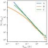 |
Fig. 4. Cumulative source counts distribution of the number of detected FRBs greater than a limiting minimum detectable peak flux density, or log N–log S plot. The resulting plots for three populations are shown here, with popA(zmax, Lbol, γ) = (0.01, 1038, 0), popB(zmax, Lbol, γ) = (2.5, 1042.5, −1.4), and popC(zmax, Lbol, γ) = (2.5, 1043, 1). Although all three populations probe very different parts of the universe, it is clear that they exhibit very similar detection parameters at high fluxes. This figure is therefore used as an illustrative example of the danger of trying to interpret the underlying intrinsic FRB population from a single log N–log S plot. |
These simulated populations have been detected with a “perfect” survey setup, allowing for instrumental effects to be decoupled from the observed source counts. Amiri et al. (2017) emphasised the fact that for cosmological populations, the brightness distribution of FRBs is not expected to be described by a single power-law, although almost all brightness distributions should asymptote towards the Euclidean scaling at high flux densities. Figure 4 demonstrates the expected behaviour; distinctions can be made between the three populations at low flux densities. On the other end, in the limit of high flux densities, these populations have similar slopes despite having very distinct intrinsic properties. While for instance plotting the spectral indices would distinguish between these populations, in the limit of high flux densities, a log N–log S plot by itself cannot do this. Figure 4 serves both as a verification of frbpoppy and as a cautionary tale for trying to interpret the underlying intrinsic FRB population from just a single distribution. This validates our use of careful population synthesis, and of using a multi-dimensional goodness-of-fit.
6.2. Event rates
While our models can be quite complex in general, particular conditions exist that simplify them and allow for direct comparison to analytical expectations. This provides a way to test our code and assumptions. As first metric for such a test, we took the detection rates that frbpoppy surveys produce. These can be tested against rather straightforward analytical scaling relationships. Connor et al. (2016b) showed that the relative FRB detection rates of surveys A and B that observe in a similar band can be expressed using the slope of the source count distribution,
 (29)
(29)
each with a detection rate R, FoV Ω, system equivalent flux density SEFD, minimum S/N, bandwidth Δν, and assuming an intrinsic slope of the source count distribution αin (see Sect. 2.1).
These scaling relationships should hold for a local non-cosmological population because their source counts are expected to be given by a single power-law. If the brightness distribution is not well described by a single power-law, the relationship between sensitivity and detection rates becomes more complicated. For example, a sensitive telescope such as Arecibo would have an advantage over less sensitive telescopes if FRBs were described by population C instead of B in Fig. 4. This is because the relative number of events falls off at low fluences in population B as the slope of the source counts flattens. Therefore, we should find that surveys probing lower fluences would see fewer FRBs than the analytical relationship would predict for a population like B. Additionally, it can help to set FRB sources to be standard candles to ensure that a similar volume is probed by both surveys. Finally, using a perfect beam pattern rather than an Airy disc prevents any beam pattern effects from playing a role in the relative FRB detection rates. Combining these premises into a Simple intrinsic population (see Table 1) and surveying this population with a range of surveys allows detection rates at various values of αin to be compared to the analytical expectations from Eq. (29). Such a comparison is made in Fig. 5 for “palfa” and “askap-fly” relative to those of “htru” as a function of αin. The expected analytical relationship is shown as dotted lines, with the results from frbpoppy overplotted in solid lines.
 |
Fig. 5. Relative detection rates of three surveys as a function of the source count slope, αin. Detection rates are normalised to the HTRU rate, using a Euclidean universe with standard candles (Simple population, left panel), and a cosmological population with a broad luminosity function (Complex population, right panel). The dotted line is computed analytically; the solid and dashed lines are the results of frbpoppy. The real detection rate per survey is given in the centre, with solid blocks denoting the 1σ Poissonian error bars (real population, centre). |
The simulated results from the Simple model match the analytical expectations very well, showing that frbpoppy acts as expected within understandable conditions. Furthermore, the change in detection rate over αin for “palfa” agrees with prior expectations from Amiri et al. (2017). The slight deviation from the trend around αin = −2.1 for “askap-fly” is solely due to insufficient detections, with larger populations eliminating this effect. Based on these results from these test cases, we conclude that generating and surveying FRB populations frbpoppy works as expected. This paves the way for more complex behaviour to be tested, as we show below.
One metric that is influenced by important and diverse elements such as the source number density, the luminosities, and the telescope modelling, whether in sensitivity, beam pattern, or other detection parameters, is the detection rate. Comparing simulated detection rates to real ones is therefore an important test of our population synthesis. To this end, the real detection rates of “palfa”, “htru”, and “askap-fly” are plotted in the centre of Fig. 5 using short horizontal lines. The surrounding blocks denote the first-order Poissonian error bars for each survey. These real detection rates can be used to constrain expected detection rates, and hence the underlying number density slope. The left panel of Fig. 5 makes clear that even with simple analytic models and a simple and well-defined source-count falloff such that α = αin, in 1.3 < |α|< 1.5 the observed FRB rates of the three main surveys are reproduced. We take this and the replication of the analytical expectations as evidence that the fundamental simulation and detection numbers in frbpoppy are correct and trustworthy.
We subsequently move to the more physically meaningful regime, leaving behind the oversimplification of the Simple population, and shifting to a Complex intrinsic FRB population. The effects of adopting this population are shown in the right panel of Fig. 5. The dashed lines denote the detection rates for a variety of simulated surveys. In Table 1 we provide an overview of the initial input parameters for this Complex population. Having stepped away from a Simple population, the interpretation of αin also changes. As described in Sect. 2.1, αin is only equal to the slope of log N–log Sα for a Euclidean universe, in all other cases, αin becomes the value to which α asymptotes in the limit of high fluences.
We chose to model the Complex population by including dispersion measure contributions, a range of luminosities rather than a standard candle, and also a negative spectral index similar to the Galactic pulsar population. Additionally, we adapted surveys to use Airy disc beam patterns with a single side lobe.
Figure 5 shows that the relative “askap-fly”/“htru” detection rates increase while the “palfa” detection rate drops significantly at high values of αin and loosens its constraints. As a result, the expected range for αin is pushed towards 1.5 < |αin|< 2.0. This range of values for αin corresponds a value for β < 1 (see Eq. (6)). Therefore we expect the comoving FRB source density to drop off towards higher redshift, indicating an evolution in the number of FRB sources. This implies that FRB sources in the early universe were less common than in the later stages of the universe, which could help in determining the FRB progenitors to an astrophysical source class. Extending these simulations to “askap-incoh” can be used to predict the expected change in ASKAP detection rates. This is shown in Fig. 6, using a similar setup to the right panel of Fig. 5. In this case, the choice is made to limit the surveys to “htru”, “askap-fly”, and “askap-incoh”, of which more details are listed in Table 2. Comparisons to real rates can be made using Fig. 5, which are additionally applicable to Fig. 6.
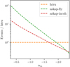 |
Fig. 6. Simulated relative detection rates for ASKAP in fly’s-eye mode (“askap-fly”) and in an incoherent mode (“askap-incoh”) scaled to “htru” and plotted against the source count slope, αin. A Complex model of the intrinsic FRB population has been used, with both surveys modelled with an Airy disc with a single side lobe. |
6.3. Distributions
A crucial first step for any simulation is its ability to replicate the observed results; the second step is to adjust the input model to maximise the quality of this replication and thus understand the input astrophysics. Our replicated parameter space includes many variables, as described in Sect. 5.2.
Here we show a comparison of just two parameters, fluence and dispersion measure, that provide an approximate measure of brightness and distance, respectively. We compare simulated and observed fluence and dispersion measure distributions from Parkes and ASKAP. The resulting plot for Parkes is shwon in Fig. 7 and for ASKAP in Fig. 8. In order to obtain these results, we surveyed a Complex intrinsic FRB population with a “parkes” survey using the Parkes beam pattern, and with an “askap-fly” model using an Airy disc with a single side lobe. More details on the intrinsic population are listed in Table 1, information on the survey parameters is added in Table 2, and an idea of the Parkes beam pattern is provided in Fig. 3.
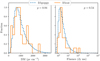 |
Fig. 7. Comparison of simulated frbpoppy and real frbcat distributions for FRB detections at Parkes. Left: dispersion measure distributions; right: fluence distributions for the same populations as the left-hand panel. frbpoppy simulations have been run on a Complex intrinsic FRB population, with the “parkes” survey modelled using the beam pattern as shown in Fig. 3. The p-value of a simple KS-test between both distributions is shown in the upper right corner of both panels. The product of these values showing the total goodness-of-fit is p = 0.51. The input parameters do not reflect the optimum values for the best fits between frbpoppy and frbcat distributions, but are merely an initial guess at some of the underlying parameters. |
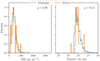 |
Fig. 8. Following Fig. 7, frbpoppy and frbcat dispersion measure and fluence ASKAP distributions. The frbpoppy populations use aComplex intrinsic FRB population and are surveyed with “askap-fly” and including a single side lobe. The total goodness-of-fit is p = 0.12. |
Figures 7 and 8 show that the broad trends of the resulting frbpoppy distributions are quite similar to those from FRBCAT, with KS-test values of p = 0.51 for the Parkes results and p = 0.12 for ASKAP. Not only does this support the capability of frbpoppy to reproduce observed data, it also shows that the Complex population parameters are favourable for exploring the intrinsic population parameter space. In comparison, a Simple population for instance was unable to reproduce the observed fluence and dispersion measure distribution. A comparison of the inputs to the two populations as given in Table 1 shows a number of key differences. A number of parameters proved crucial for replicating real detections. Both the cosmological nature of the Complex population, in obtaining a good match to observed data, and the lognormal nature of the pulse width distribution proved to be important factors. This shows that the intrinsic FRB population is more complex and varied than admittedly tempting simple approximations of the intrinsic population. Note there is a sampling difference between frbpoppy and FRBCAT, as the latter comprises tens of FRBs, and frbpoppy showing hundreds. With additional real FRB observations, the constraints on the intrinsic FRB population could be tighter.
6.4. Beam patterns
In general, the telescopes simulated in this work are most sensitive at boresight, and they are well understood there. Away from this beam centre, however, the sensitivity of an observation can be quickly reduced, as shown in Fig. 2, and the exact shape of the fall-off becomes important. The beam pattern of telescopes such as Parkes is not well known at large angular distances from the boresight. Adopting for instance an Airy disc with a large number of side lobes might skew any resulting distributions towards brighter FRBs, with dim FRBs less likely to be detected. In Fig. 9 we show an example of the change in observed DM distributions based on the choice of beam pattern. Where with a perfect beam pattern, the simulated observed distribution is found to peak towards higher DM values, an Airy or Gaussian profile shifts the peak leftwards, to lower DMs. More noticeable is the left shoulder of the Airy disc with four side lobes, which appears to suggest a far steeper build-up of FRB sources at low DMs despite the “perfect” beam showing otherwise. If beam pattern effects are not properly taken into account, they will easily lead to erroneous conclusions about the intrinsic number density of FRBs. Additionally, this behaviour could complicate comparisons between surveys, which each have their own unique beam pattern effect convolved within their detections. In Fig. 9 the input parameters were chosen to best illustrate these effects, using a Standard Candle population (see Table 1) being observed with a perfect telescope setup (see Table 2). This survey was adapted to feature a smaller FoV of 10 deg2 and detections made for a peak flux density Speak > 10−10 Jy. Shifting the detection threshold causes the effects shown in Fig. 9 to become less noticeable, but they are still present.
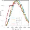 |
Fig. 9. Relative fraction of FRB detections over dispersion measure for a variety of beam patterns. In this case, airy-0 and airy-4 denote an Airy disc without side lobes and one with four side lobes. The FRBs were simulated with the Standard Candle class parameters. |
7. Discussion
7.1. Caveats
Most scientific models have a wide range of caveats, with frbpoppy being no exception to this rule. We attempt to address some of these caveats below.
7.1.1. Repeaters
As described in Sect. 2, this first version of frbpoppy models FRBs as one-off events, even though repeating FRBs have been detected. The reasons for this choice were that firstly, it would be difficult to do population statistics including repeaters because at this stage, only a handful of repeaters are known. Secondly, should both a repeater and a true one-off population underlie the observed FRBs, then our results would still hold for the one-off population. This assumes that there would be a way to distinguish between both populations because otherwise contamination between the two populations would prohibit separate modelling. The potentially long repetition timescale of repeater sources may indeed allow modelling FRBs as one-off sources. Then only the number of pulses emitted over an FRB lifetime needs to be taken into account when the FRB number density is converted (Sect. 2.1) to a birth rate. Nonetheless, repeaters are being included in the future version of frbpoppy, and they are subject to further synthesis research. This will allow for characterising the fraction of repeating to non-repeating FRB sources, and potentially their progenitor populations.
7.1.2. Beam patterns
As we showed in Sect. 6.4, determining the beam pattern is essential for understanding the results of any survey. Actual beam patterns are rarely ideal, as is strikingly clear from the differences between Figs. 2 and 3.
Furthermore, cylindrical telescopes such as UTMOST or CHIME have complex, elongated beam patterns (cf. Bailes et al. 2017). The results in Fig. 9 demonstrate the importance of knowing the survey beam pattern because the effects on resulting detections can be important. To ensure that FRB detections from various surveys can be compared against each other, it is important that surveys release not just survey parameters, but also a map of their beam pattern. Doing so will significantly improve the constraints that surveys can place on the intrinsic FRB population.
While for pulsar population studies the beam pattern is in principle the same, the effects of the side lobes are generally of much more consequence in FRB studies. Because side lobes generally rotate on the sky, their effects wash out during the relatively long integrations used in the periodicity when searching for pulsars. Then only the central, axisymmetric parts of the beam shape add to a detection. For FRB and other single-pulse searches, the instantaneous beam pattern, including any strong side lobes, is more important.
7.1.3. Fluence limits
One of the strengths of population synthesis is tracking down detection biases. One such bias, as described in Keane & Petroff (2015), lies within the fluence space. Two FRBs could have the same fluence, and yet only one might be detected if their pulse widths differ, for example. Thus sampling the fluences of an FRB population will show an incomplete picture. A commonly used method to ensure some form of completeness is shifting to the Speak–weff space and using a fluence completeness-limit. By rewriting Eq. (17), we can decide to use FRBs only when they lie above a particular constant fluence and below a maximum weff (see e.g. Fig. 2 of Keane & Petroff 2015). While this can indeed prevent fluence incompleteness, it thereby overlooks other FRBs. We replicate this incompleteness in frbpoppy using a simple S/N detection threshold, as surveys often do. The S/N threshold rather than a fluence completeness limit the frbpoppy survey detections shows the bias in the fluence space, which necessarily is an incomplete sampling of the parameter space. Knowledge of the underlying pulse width distribution would help map out the extent of the selection effects mentioned in this paragraph, but this may not be achievable in the near future.
7.1.4. Software selection effects
In generating our simulated observed surveys, we took care to model a number of boundaries to the FRB search parameter space. For the telescope hardware system, these are usually well described; for the software, this is not always the case. We therefore modelled in frbpoppy the minimum sampling time, but not the maximum searched pulse widths, and we modelled the intra-channel DM smearing, but not the search DM-step smearing. Some care with simulation inputs is therefore advised to ensure that the simulated detections remain well within the bounds of any software selection effects. In general, a number of search-software selection effects exist that are beyond the scope of the current work. Several research teams are pursuing a more thorough investigation of this FRB search-software completeness and bias in separate lines of research (Mendrik & Hester, in prep.; Connor et al., in prep.).
7.2. Comparing population synthesis for FRBs with that for pulsars
The current research, and frbpoppy, follow from population synthesis work in the pulsar community through for example the open-source psrpoppy code. While there are a number of similarities, these are offset by some intrinsic differences. In both cases, large numbers of sources need to be generated. In the pulsar population synthesis of van Leeuwen & Stappers (2010), for example, the generated population sizes in a run from a single parameter set is generally 107 pulsars. For about 5 × 10⁵ of these, the full orbit through the galaxy was simulated, a task frbpoppy does not need to perform. Searching through multiple parameters generally runs on clusters (or very large servers). An FRB population quickly starts running into intrinsic populations of 108 FRBs.
One main difference is, however, that already when pulsar population synthesis research began, neutron stars were known to be the source class. Furthermore, a significant number had been localised and their distances determined, and their intrinsic brightnesses were therefore well understood. In contrast, with FRBs we find a lack of understanding on the intrinsic emission properties. This makes the parameter space over which FRBs have to be modelled significantly larger than that for pulsars.
A further key difference between FRB and pulsar population synthesis is their respective one-off and periodic burst properties. In an all-sky survey, a pulsar that is always on will be detected most brightly in the pointing where the main beam points closest to it. For FRBs this is not so. They are most likely not emitting in that optimally directed pointing. Most FRBs will burst while covered by the larger side lobes. And emitting FRB is thus more dependant on its placement within a beam pattern, with only a single chance to detect one-off sources. This also severely affects the detection rates in comparison to pulsars: FRBs that emit outside of a beam pattern are gone for ever.
7.3. Comparing frbpoppy results with other FRB simulations
We have investigated how to compare results from frbpoppy with those from the population synthesis studies listed in Sect. 1. Direct comparisons are hampered by the different scope of the simulations and the rapidly changing datasets. Caleb et al. (2016a), for example, focused on nine HTRU events, with few other data being available at the time. For the generation of their FRB populations, a similar path to frbpoppy was taken, testing several cosmological models, adopting a linear DM-z relationship and a range of telescope selection effects. A number of fundamental differences in approach also exist, however, such as the treatment of the spectral index, and adopting scattering relationships. Nonetheless, similar results were obtained in terms of fluence and dispersion measure distributions, with frbpoppy showing a slightly better fit to Parkes detections, (pfrbpoppy = 0.51 versus pCaleb et al. = 0.03). If the Caleb et al. (2016a) research were extended to the current detections (beyond the scope of the current paper), it could be more directly compared to frbpoppy. Facilitating such comparisons is one of the drivers for making frbpoppy open source.
7.4. Event rates
The FRB event rates can be difficult to interpret (Connor et al. 2016b). The rate at which an individual survey detects bursts is the simplest to calculate. It is more difficult to convert that number into an all-sky rate because this requires good knowledge of the telescope beam pattern and the FRB brightness distribution (Macquart & Ekers 2018b). It is harder still to produce a volumetric event rate because this requires information about the spatial distribution of FRBs, and without redshifts for large numbers of sources, the volume of space occupied by FRBs is degenerate with their repetition statistics and luminosity function. Of course, localisations such as those by ASKAP (e.g. Bannister et al. 2019) help determining a volumetric rate, providing a redshift, and thereby a handle on the luminosity function etc.
While it is the most difficult to constrain, the volumetric rate is the most informative quantity because it contains information about the progenitor population. Given the difficulty of inverting a detection rate into a rate on the sky and then a volumetric rate, running a large Markov chain Monte Carlo (MCMC) simulation with frbpoppy is the best approach to constraining the frequency at which cosmological FRBs are produced. frbpoppy handles beam effects and instrumental biases, and given enough resources, the code can answer the question which volumetric event rates are consistent with current data. Therefore, it is promising that we have already shown the consistency between both absolute detection rates in frbpoppy and the relative event rates between surveys, for example in Fig. 5. Additionally, current detection rates constraining |αin|> 1.5 for a Complex population point towards a possible evolution of FRB sources: more occur per unit comoving volume in the nearby universe than in the distant universe.
7.5. Observed distributions
In Figs. 7 and 8 we showed that our simulated parameter distributions agree well with the observed ones for the Complex population. The properties of this model therefore warrant further examination. Starting with the number density, Table 1 shows the population following a comoving volume density, rather than SFR. This choice was made so that the intrinsic number density could vary with αin, and does not de facto rule out other number densities from being able to fit the data. The fits as shown in Fig. 5 indicate some form of evolution in the FRB progenitor population. We cannot rule out a Euclidean distribution with the current data, however. We will further explore the evolution of FRB progenitors in future work. This might allow current detections to tie FRBs to a progenitor population.
Additionally, the simulated population extends out to a redshift of 2.5, which leads to a choice of intrinsic bolometric luminosity of 1039 − 1045 ergs s−1. Varying both the maximum redshift and the luminosities can result in a similar population (see Fig. 4), therefore setting one of the two parameters helps set the other when a representative outcome is the aim. In the case of the distributions discussed here, the simulated luminosities agree with Yang et al. (2017), who advocated a luminosity around L ∼ 1043 ergs s−1 with a narrow spread. The chosen luminosity range subsequently informs the choice of intrinsic pulse widths, which were drawn from a log-normal distribution. In future frbpoppy runs, information from repeater sources could help inform the choice of pulse width distributions. Additional constraints could be placed using the pulse width distribution of detected FRBs if the strength of the pulse-broadening effects in the host galaxy and intergalactic medium are well understood.
The strength of pulse-broadening effects ties into the choice of intergalactic dispersion measure. While initial research suggested a first-order approximation of DMIGM ∼ 1200z with redshift z (Inoue 2004), more recent treatments tend towards a smaller scaling factor between 800 and 1000 pc cm3 (Zhang 2018; Keane 2018; Pol et al. 2019). We chose a simple relation of 1000 pc cm3 and a DMIGM drawn from a Gaussian centred around 100 pc cm3, until information from both repeater sources, and improved localisations further constrain these values. We acknowledge that a more accurate relation could be obtained using non-linear relationships (see Batten 2019), and may indeed be important at the redshift of HeII ionisation. Implementing such relationships directly in frbpoppy would significantly increase the computation time, however, and some form of pre-optimisation would have to be implemented.
Difficulties in measuring a spectral index γ make setting this value challenging. Currently set to follow the spectral index seen in pulsars, with a value of −1.4 (Bates et al. 2013), a diverse range of predictions are present in the literature. Where for instance Macquart et al. (2019) argued for a steep negative spectral index, Farah et al. (2019) suggested a possible spectral turnover in line with Ravi & Loeb (2019). Further muddling the idea of a spectral index are repeater observations that present indications that FRBs are emitted in emission envelops (e.g. Gourdji et al. 2019; Hessels et al. 2019). Testing a variety of relationships between the FRB source energy and frequency would help in this regard, and could be taken into consideration in future work. In any case, additional measurements of FRB spectral index (or shape) would help inform the choice of γ within frbpoppy. As we showed in the limit of low fluences in Fig. 4, the spectral index affects the brightness distributions, and can help distinguish between intrinsic populations.
There are two obvious avenues to explore in future work on the distributions generated by frbpoppy: simulating more variations on the intrinsic populations, and expanding the number of parameters that are fit in the code. Both paths will improve constraints on the intrinsic FRB population. The increase in FRB detections from new surveys will also make for better comparisons by constraining the physical parameter space occupied by the real population. It is clear that while our current inputs can explain the observed FRB population, frbpoppy provides fertile ground for further constraining the intrinsic FRB population.
7.6. Opportunities, uses, and future work
The open-source nature of frbpoppy is meant to encourage survey teams to update their survey parameters and add descriptions of new search efforts. The main goal, however, is to allow an open platform for FRB population synthesis so that research teams can analyse the effect of new discoveries. These can range from new algorithms for generating populations to new diagnostic plots for investigating FRB properties.
We demonstratec the basic frbpoppy functionality here, and our next goals are to simulate the influence of a number of physical unknowns. We thereby aim to investigate their effects on our simulated population, and from inverting the real population, determine how important these physical unknowns are.
Immediate examples of these unknowns are whether the FRB birth rate follows the SFR or is flat; what the fraction of repeating FRBs is; and how many FRBs are broad-band emitters. All these will be strongly guided by the continuing results from existing and new surveys.
8. Conclusions
We have developed frbpoppy, an open-source Python package capable of conducting a fast radio burst population synthesis. Using this software, we can replicate observed FRB detection rates and FRB distributions. frbpoppy does this in three steps that we describe below.
-
frbpoppy starts by simulating a cosmic population of one-off FRBs, for which a user can choose from a wide range of options, including models for source number density, cosmology, host DM, intergalactic medium DM, Milky Way DM, luminosity functions, emission bands, pulse widths, spectral indices, and choices for the maximum redshift and size of the FRB population. These are merely a selection of the frontend options, and more options are available within frbpoppy.
-
frbpoppy then generates a survey by adopting a beam pattern and using survey parameters such as the telescope gain, sampling time, receiver temperature, central frequency, bandwidth, channel bandwidth, number of polarisations, FoV, S/N limit, and any survey region limits.
-
In the final step, frbpoppy convolves the generated intrinsic population with the generated survey to simulate an observed FRB population.
By testing frbpoppy, we showed that the FRB detection rates of ASKAP, Parkes, and Arecibo can be reproduced, as can the observed fluence and dispersion measure distributions of ASKAP and Parkes. These observed results are replicated best by our “Complex model” (multiple DM contributions, range of luminosities, and negative spectral index). Overall, this enables predictions to be made about the detection rates of future surveys, and about the intrinsic FRB population. We demonstrated the importance of understanding the beam pattern of a survey by comparing the effects of various beam patterns. Future work will focus on auto-iteration over input parameters, on FRB repetition, and on further constraining the intrinsic FRB population.
For a full list of published FRBs, see the FRB Catalogue: www.frbcat.org (Petroff et al. 2016).
Acknowledgments
We thank Chris Flynn for carefully reading this manuscript and for providing valuable comment and suggestions. We also thank the participants of the 2017−2019 FRB meetings for the useful discussions. Thanks additionally go to Sarah Burke-Spolaor for initial survey parameter data. DWG acknowledges travel support from the Research Corporation for Scientific Advancement to attend the Aspen FRB meeting in 2017. The research leading to these results has received funding from the European Research Council under the European Union’s Seventh Framework Programme (FP/2007-2013)/ERC Grant Agreement n. 617199 (“ALERT”); from Vici research programme “ARGO” with project number 639.043.815, financed by the Netherlands Organisation for Scientific Research (NWO); and from the Netherlands Research School for Astronomy (NOVA4-ARTS). EP further acknowledges funding from an NWO Veni Fellowship. This research has made use of numpy (van der Walt et al. 2011), scipy (Oliphant 2007), astropy (Astropy Collaboration 2018), matplotlib (Hunter 2007), bokeh (Bokeh Development Team 2018) and NASA’s Astrophysics Data System.
References
- Adams, E. A. K., & van Leeuwen, J. 2019, Nat. Astron., 3, 188 [NASA ADS] [CrossRef] [Google Scholar]
- Amiri, M., Bandura, K., Berger, P., et al. 2017, ApJ, 844, 161 [NASA ADS] [CrossRef] [Google Scholar]
- Astropy Collaboration (Price-Whelan, A. M., et al.) 2018, AJ, 156, 123 [Google Scholar]
- Bailes, M., Jameson, A., Flynn, C., et al. 2017, PASA, 34, e045 [NASA ADS] [CrossRef] [Google Scholar]
- Bannister, K. W., Shannon, R. M., Macquart, J. P., et al. 2017, ApJ, 841, L12 [NASA ADS] [CrossRef] [Google Scholar]
- Bannister, K. W., Deller, A. T., Phillips, C., et al. 2019, Science, 365, 565 [NASA ADS] [CrossRef] [Google Scholar]
- Bates, S. D., Lorimer, D. R., & Verbiest, J. P. W. 2013, MNRAS, 431, 1352 [NASA ADS] [CrossRef] [Google Scholar]
- Bates, S. D., Lorimer, D. R., Rane, A., & Swiggum, J. 2014, MNRAS, 439, 2893 [NASA ADS] [CrossRef] [Google Scholar]
- Bates, S. D., Lorimer, D. R., Rane, A., & Swiggum, J. 2015, Astrophysics Source Code Library [record ascl:1501.006] [Google Scholar]
- Batten, A. 2019, J. Open Source Softw., 4, 1399 [NASA ADS] [CrossRef] [Google Scholar]
- Beloborodov, A. M. 2019, ApJ, submitted [arXiv:1908.07743] [Google Scholar]
- Bhat, N. D. R., Cordes, J. M., Camilo, F., Nice, D. J., & Lorimer, D. R. 2004, ApJ, 605, 759 [CrossRef] [Google Scholar]
- Bhattacharya, D., Wijers, R. A. M. J., Hartman, J. W., & Verbunt, F. 1992, A&A, 254, 198 [NASA ADS] [Google Scholar]
- Bhattacharya, M., Kumar, P., & Lorimer, D. 2019, MNRAS, submitted [arXiv:1902.10225] [Google Scholar]
- Bokeh Development Team 2018, Bokeh: Python Library for Interactive Visualization [Google Scholar]
- Caleb, M., Flynn, C., Bailes, M., et al. 2016a, MNRAS, 458, 708 [NASA ADS] [CrossRef] [Google Scholar]
- Caleb, M., Flynn, C., Bailes, M., et al. 2016b, MNRAS, 458, 718 [NASA ADS] [CrossRef] [Google Scholar]
- Caleb, M., Stappers, B. W., Rajwade, K., & Flynn, C. 2019, MNRAS, 484, 5500 [NASA ADS] [CrossRef] [Google Scholar]
- Champion, D. J., Petroff, E., Kramer, M., et al. 2016, MNRAS, 460, L30 [NASA ADS] [CrossRef] [Google Scholar]
- Chawla, P., Kaspi, V. M., Josephy, A., et al. 2017, ApJ, 844, 140 [NASA ADS] [CrossRef] [Google Scholar]
- Chippendale, A. P., Brown, A. J., Beresford, R. J., et al. 2015, 2015 International Conference on Electromagnetics in Advanced Applications (ICEAA), 541 [CrossRef] [Google Scholar]
- Connor, L. 2019, MNRAS, 487, 5753 [NASA ADS] [CrossRef] [Google Scholar]
- Connor, L., Sievers, J., & Pen, U.-L. 2016a, MNRAS, 458, L19 [Google Scholar]
- Connor, L., Lin, H.-H., Masui, K., et al. 2016b, MNRAS, 460, 1054 [NASA ADS] [CrossRef] [Google Scholar]
- Cordes, J. M., & Lazio, T. J. W. 2002, ArXiv e-prints [arXiv:astro-ph/0207156] [Google Scholar]
- Cordes, J. M., & Lazio, T. J. W. 2003, ArXiv e-prints [arXiv:astro-ph/0301598] [Google Scholar]
- Cordes, J. M., & McLaughlin, M. A. 2003, ApJ, 596, 1142 [NASA ADS] [CrossRef] [Google Scholar]
- Cordes, J. M., & Wasserman, I. 2016, MNRAS, 457, 232 [NASA ADS] [CrossRef] [Google Scholar]
- Cordes, J. M., Freire, P. C. C., Lorimer, D. R., et al. 2006, ApJ, 637, 446 [NASA ADS] [CrossRef] [Google Scholar]
- Farah, W., Flynn, C., Bailes, M., et al. 2018, MNRAS, 478, 1209 [NASA ADS] [CrossRef] [Google Scholar]
- Farah, W., Flynn, C., Bailes, M., et al. 2019, MNRAS, 488, 2989 [Google Scholar]
- Faucher-Giguère, C.-A., & Kaspi, V. M. 2006, ApJ, 643, 332 [NASA ADS] [CrossRef] [Google Scholar]
- Fialkov, A., Loeb, A., & Lorimer, D. R. 2018, ApJ, 863, 132 [NASA ADS] [CrossRef] [Google Scholar]
- Ghirlanda, G., Ghisellini, G., Salvaterra, R., et al. 2013, MNRAS, 428, 1410 [NASA ADS] [CrossRef] [EDP Sciences] [Google Scholar]
- Gourdji, K., Michilli, D., Spitler, L. G., et al. 2019, ApJ, 877, L19 [NASA ADS] [CrossRef] [Google Scholar]
- Gunn, J. E., & Ostriker, J. P. 1970, ApJ, 160, 979 [NASA ADS] [CrossRef] [Google Scholar]
- Hessels, J. W. T., Spitler, L. G., Seymour, A. D., et al. 2019, ApJ, 876, L23 [NASA ADS] [CrossRef] [Google Scholar]
- Hewish, A., Bell, S. J., Pilkington, J. D. H., Scott, P. F., & Collins, R. A. 1968, Nature, 217, 709 [NASA ADS] [CrossRef] [Google Scholar]
- Hogg, D. W. 1999, ArXiv e-prints [arXiv:astro-ph/9905116] [Google Scholar]
- Hunter, J. D. 2007, Comput. Sci. Eng., 9, 90 [NASA ADS] [CrossRef] [Google Scholar]
- Inoue, S. 2004, MNRAS, 348, 999 [NASA ADS] [CrossRef] [Google Scholar]
- Ioka, K. 2003, ApJ, 598, L79 [NASA ADS] [CrossRef] [Google Scholar]
- Izzard, R. G., & Halabi, G. M. 2018, ArXiv e-prints [arXiv:1808.06883] [Google Scholar]
- Johnson, N. 1994, Continuous Univariate Distributions (New York: Wiley) [Google Scholar]
- Katz, J. I. 2014, Phys. Rev. D, 89, 103009 [NASA ADS] [CrossRef] [Google Scholar]
- Keane, E. F. 2018, Nat. Astron., 2, 865 [NASA ADS] [CrossRef] [Google Scholar]
- Keane, E. F., & Petroff, E. 2015, MNRAS, 447, 2852 [NASA ADS] [CrossRef] [Google Scholar]
- Keith, M. J., Jameson, A., van Straten, W., et al. 2010, MNRAS, 409, 619 [NASA ADS] [CrossRef] [Google Scholar]
- Lazarus, P., Brazier, A., Hessels, J. W. T., et al. 2015, ApJ, 812, 81 [NASA ADS] [CrossRef] [Google Scholar]
- Lorimer, D. 2011, Astrophysics Source Code Library [record ascl:1107.019] [Google Scholar]
- Lorimer, D. R., & Kramer, M. 2012, Handbook of Pulsar Astronomy (Cambridge: Cambridge University Press) [Google Scholar]
- Lorimer, D. R., Faulkner, A. J., Lyne, A. G., et al. 2006, MNRAS, 372, 777 [NASA ADS] [CrossRef] [Google Scholar]
- Lorimer, D. R., Bailes, M., McLaughlin, M. A., Narkevic, D. J., & Crawford, F. 2007, Science, 318, 777 [NASA ADS] [CrossRef] [PubMed] [Google Scholar]
- Lorimer, D. R., Karastergiou, A., McLaughlin, M. A., & Johnston, S. 2013, MNRAS, 436, L5 [NASA ADS] [CrossRef] [Google Scholar]
- Lu, W., & Kumar, P. 2018, MNRAS, 477, 2470 [NASA ADS] [CrossRef] [Google Scholar]
- Luo, R., Lee, K., Lorimer, D. R., & Zhang, B. 2018, MNRAS, 481, 2320 [NASA ADS] [CrossRef] [Google Scholar]
- Lyne, A. G., Manchester, R. N., & Taylor, J. H. 1985, MNRAS, 213, 613 [NASA ADS] [CrossRef] [Google Scholar]
- Maan, Y., & van Leeuwen, J. 2017, ArXiv e-prints [arXiv:1709.06104] [Google Scholar]
- Macquart, J.-P., & Ekers, R. 2018a, MNRAS, 480, 4211 [NASA ADS] [CrossRef] [Google Scholar]
- Macquart, J.-P., & Ekers, R. D. 2018b, MNRAS, 474, 1900 [NASA ADS] [CrossRef] [Google Scholar]
- Macquart, J.-P., & Koay, J. Y. 2013, ApJ, 776, 125 [NASA ADS] [CrossRef] [Google Scholar]
- Macquart, J. P., Shannon, R. M., Bannister, K. W., et al. 2019, ApJ, 872, L19 [NASA ADS] [CrossRef] [Google Scholar]
- Madau, P., & Dickinson, M. 2014, ARA&A, 52, 415 [NASA ADS] [CrossRef] [Google Scholar]
- Masui, K. W., & Sigurdson, K. 2015, Phys. Rev. Lett., 115, 121301 [NASA ADS] [CrossRef] [Google Scholar]
- Masui, K., Lin, H.-H., Sievers, J., et al. 2015, Nature, 528, 523 [NASA ADS] [CrossRef] [Google Scholar]
- McQuinn, M. 2014, ApJ, 780, L33 [NASA ADS] [CrossRef] [Google Scholar]
- Metzger, B. D., Margalit, B., & Sironi, L. 2019, MNRAS, 485, 4091 [NASA ADS] [CrossRef] [Google Scholar]
- Michilli, D., Seymour, A., Hessels, J. W. T., et al. 2018, Nature, 553, 182 [NASA ADS] [CrossRef] [Google Scholar]
- Narayan, R., & Ostriker, J. P. 1990, ApJ, 352, 222 [NASA ADS] [CrossRef] [Google Scholar]
- Niino, Y. 2018, ApJ, 858, 4 [NASA ADS] [CrossRef] [Google Scholar]
- Oliphant, T. E. 2007, Comput. Sci. Eng., 9, 10 [CrossRef] [PubMed] [Google Scholar]
- Oosterloo, T., Verheijen, M. A. W., van Cappellen, W., et al. 2009, Wide Field Astronomy& Technology for the Square Kilometre Array, 70 [Google Scholar]
- Oppermann, N., Connor, L. D., & Pen, U.-L. 2016, MNRAS, 461, 984 [NASA ADS] [CrossRef] [Google Scholar]
- Patel, C., Agarwal, D., Bhardwaj, M., et al. 2018, ApJ, 869, 181 [NASA ADS] [CrossRef] [Google Scholar]
- Petroff, E., Johnston, S., Keane, E. F., et al. 2015, MNRAS, 454, 457 [NASA ADS] [CrossRef] [Google Scholar]
- Petroff, E., Barr, E. D., Jameson, A., et al. 2016, PASA, 33, e045 [NASA ADS] [CrossRef] [Google Scholar]
- Petroff, E., Hessels, J. W. T., & Lorimer, D. R. 2019, A&ARv, 27, 4 [NASA ADS] [CrossRef] [Google Scholar]
- Planck Collaboration XIII. 2016, A&A, 594, A13 [NASA ADS] [CrossRef] [EDP Sciences] [Google Scholar]
- Platts, E., Weltman, A., Walters, A., et al. 2019, Phys. Rep., 821, 1 [NASA ADS] [CrossRef] [Google Scholar]
- Pol, N., Lam, M. T., McLaughlin, M. A., Lazio, T. J. W., & Cordes, J. M. 2019, ApJ, submitted [arXiv:1903.07630] [Google Scholar]
- Ravi, V. 2019, Nat. Astron., 3, 928 [NASA ADS] [CrossRef] [Google Scholar]
- Ravi, V., & Loeb, A. 2019, ApJ, 874, 72 [NASA ADS] [CrossRef] [Google Scholar]
- Ravi, V., Shannon, R. M., Bailes, M., et al. 2016, Science, 354, 1249 [NASA ADS] [CrossRef] [Google Scholar]
- Ravi, V., Catha, M., D’Addario, L., et al. 2019a, Nature, 572, 352 [NASA ADS] [CrossRef] [Google Scholar]
- Ravi, V., Battaglia, N., Burke-Spolaor, S., et al. 2019b, BAAS, 51, 420 [Google Scholar]
- Remazeilles, M., Dickinson, C., Banday, A. J., Bigot-Sazy, M. A., & Ghosh, T. 2015, MNRAS, 451, 4311 [NASA ADS] [CrossRef] [Google Scholar]
- Romero, G. E., del Valle, M. V., & Vieyro, F. L. 2016, Phys. Rev. D, 93, 023001 [NASA ADS] [CrossRef] [Google Scholar]
- Sanidas, S., Cooper, S., Bassa, C. G., et al. 2019, A&A, 626, A104 [NASA ADS] [CrossRef] [EDP Sciences] [Google Scholar]
- Scholz, P., Spitler, L. G., Hessels, J. W. T., et al. 2016, ApJ, 833, 177 [NASA ADS] [CrossRef] [Google Scholar]
- Shannon, R. M., Macquart, J. P., Bannister, K. W., et al. 2018, Nature, 562, 386 [NASA ADS] [CrossRef] [Google Scholar]
- Smits, R., Kramer, M., Stappers, B., et al. 2009, A&A, 493, 1161 [NASA ADS] [CrossRef] [EDP Sciences] [Google Scholar]
- Spitler, L. G., Cordes, J. M., Hessels, J. W. T., et al. 2014, ApJ, 790, 101 [NASA ADS] [CrossRef] [Google Scholar]
- Spitler, L. G., Scholz, P., Hessels, J. W. T., et al. 2016, Nature, 531, 202 [NASA ADS] [CrossRef] [Google Scholar]
- Szary, A., Zhang, B., Melikidze, G. I., Gil, J., & Xu, R.-X. 2014, ApJ, 784, 59 [NASA ADS] [CrossRef] [Google Scholar]
- Taylor, J. H., & Manchester, R. N. 1977, ApJ, 215, 885 [NASA ADS] [CrossRef] [Google Scholar]
- Tendulkar, S. P., Bassa, C. G., Cordes, J. M., et al. 2017, ApJ, 834, L7 [NASA ADS] [CrossRef] [Google Scholar]
- The CHIME/FRB Collaboration (Amiri, M., et al.) 2018, ApJ, 863, 48 [NASA ADS] [CrossRef] [Google Scholar]
- The CHIME/FRB Collaboration (Amiri, M., et al.) 2019, Nature, 566, 235 [NASA ADS] [CrossRef] [Google Scholar]
- Thompson, A. R., Moran, J. M., & Swenson, Jr., G. W. 2017, Interferometry and Synthesis in Radio Astronomy, 3rd Edition (Krieger Publishing Company) [CrossRef] [Google Scholar]
- Thornton, D., Stappers, B., Bailes, M., et al. 2013, Science, 341, 53 [NASA ADS] [CrossRef] [PubMed] [Google Scholar]
- van der Walt, S., Colbert, S. C., & Varoquaux, G. 2011, Comput. Sci. Eng., 13, 22 [Google Scholar]
- van Leeuwen, J., & Stappers, B. W. 2010, A&A, 509, A7 [NASA ADS] [CrossRef] [EDP Sciences] [Google Scholar]
- van Leeuwen, J., & Verbunt, F. 2004, in Young Neutron Stars and Their Environments, eds. F. Camilo, & B. M. Gaensler, IAU Symp., 218, 41 [NASA ADS] [Google Scholar]
- Vedantham, H. K., Ravi, V., Hallinan, G., & Shannon, R. M. 2016, ApJ, 830, 75 [NASA ADS] [CrossRef] [Google Scholar]
- Vieyro, F. L., Romero, G. E., Bosch-Ramon, V., Marcote, B., & del Valle, M. V. 2017, A&A, 602, A64 [NASA ADS] [CrossRef] [EDP Sciences] [Google Scholar]
- Walker, C. R. H., Ma, Y. Z., & Breton, R. P. 2018, A&A, submitted [arXiv:1804.01548] [Google Scholar]
- Wright, E. L. 2006, PASP, 118, 1711 [NASA ADS] [CrossRef] [Google Scholar]
- Xu, S., & Zhang, B. 2016, ApJ, 832, 199 [NASA ADS] [CrossRef] [Google Scholar]
- Yang, Y.-P., Luo, R., Li, Z., & Zhang, B. 2017, ApJ, 839, L25 [NASA ADS] [CrossRef] [Google Scholar]
- Yao, J. M., Manchester, R. N., & Wang, N. 2017, ApJ, 835, 29 [NASA ADS] [CrossRef] [Google Scholar]
- Zhang, B. 2018, ApJ, 867, L21 [NASA ADS] [CrossRef] [Google Scholar]
Appendix A: Beam pattern derivation
The S/N of an FRB is partially determined by its placement in the beam of a telescope. Calculating this scaling factor, henceforth referred to as the intensity profile I(r), can be a complicated task if the survey is multi-beamed. For simpler setups or single beam surveys, the intensity profile can be approximated as a Gaussian or an Airy disc. Calculating I(r) then requires just three components: the functions describing these shapes, the radial scaling of the shapes, and the maximum allowable radial offset.
An Airy disc can be described by
 (A.1)
(A.1)
with J1 the first Bessel function (Thompson et al. 2017). The scaling factor k can be expressed as follows:
 (A.2)
(A.2)
with
 (A.3)
(A.3)
where Aeff is the effective area of the beam, given by
 (A.4)
(A.4)
with c the speed of light, νc the central frequency of the survey, and D a conversion factor from arcminutes to radians, given by
 (A.5)
(A.5)
and the FWHM given by
 (A.6)
(A.6)
with the beamsize Abeam given in degrees. With
 (A.7)
(A.7)
k can be reduced to
 (A.8)
(A.8)
In a similar fashion, the radial offset N over an Airy disc can be given by
 (A.9)
(A.9)
Obtaining a radial offset requires the diameter to be halved ( ), and to ensure that the intensity profile is sampled uniformly over a disc, a
  is required. This leaves M, a scaling factor giving the maximum offset. The choice is made to set this to any of the null points of an Airy function, providing the option of choosing the number of side lobes that are to be included. To obtain the null points, the following equation can be used:
 (A.10)
Solving for n and using Eq. (A.1) allows M to be constructed as
 (A.11)
Effectively, the choice of the mth n allows choosing which side lobe is to be included. The choice is made to use the same factor for a Gaussian beam simply because the maximum offset has to be placed somewhere, and equating it to M allows for quick comparisons between results obtained with either the Gaussian or the Airy disc.
All Tables
Overview of the parameters that are required to generate an initial cosmic FRB population.
Selection of parameters that are available within frbpoppy for a surveyed FRB population.
All Figures
|
Fig. 1. Comoving number density (ρ(z)≡dN/dz) as a function of redshift from a simulated distribution of 106 FRBs. The FRBs either follow a constant number density per comoving volume element (Wright 2006), the SFR (Madau & Dickinson 2014), the SMD (Madau & Dickinson 2014), or a power law in the comoving volume space with index αin = −0.5 or αin = −2.0 (see Sect. 2.1). Note that dnFRB refers to the intrinsic number of FRBs and not to an observed number because that would be affected by a factor of (1 + z)−1 as well as the luminosity function, spectral index, etc. |
| In the text | |
|
Fig. 2. Intensity profile of various beam patterns as function of the radial offset from the centre. The relative scaling on the vertical axis is linked to selected survey’s beam size at FWHM, as calculated from beamsizes seen in Table 2. Up to eight sidelobes can be included in frbpoppy surveys, but the option to simulate a beam out to the FWHM is also possible (as illustrated by the “perfect” beam pattern). |
| In the text | |
|
Fig. 3. Shaded regions: possible beam intensities of respectively the Parkes Multibeam and Apertif Phased Array Feed (PAF) as a function of radial offset from the centre of the beam (Ravi et al. 2016; Hess, priv. comm.). Solid lines: average intensity profile per survey. |
| In the text | |
|
Fig. 4. Cumulative source counts distribution of the number of detected FRBs greater than a limiting minimum detectable peak flux density, or log N–log S plot. The resulting plots for three populations are shown here, with popA(zmax, Lbol, γ) = (0.01, 1038, 0), popB(zmax, Lbol, γ) = (2.5, 1042.5, −1.4), and popC(zmax, Lbol, γ) = (2.5, 1043, 1). Although all three populations probe very different parts of the universe, it is clear that they exhibit very similar detection parameters at high fluxes. This figure is therefore used as an illustrative example of the danger of trying to interpret the underlying intrinsic FRB population from a single log N–log S plot. |
| In the text | |
|
Fig. 5. Relative detection rates of three surveys as a function of the source count slope, αin. Detection rates are normalised to the HTRU rate, using a Euclidean universe with standard candles (Simple population, left panel), and a cosmological population with a broad luminosity function (Complex population, right panel). The dotted line is computed analytically; the solid and dashed lines are the results of frbpoppy. The real detection rate per survey is given in the centre, with solid blocks denoting the 1σ Poissonian error bars (real population, centre). |
| In the text | |
|
Fig. 6. Simulated relative detection rates for ASKAP in fly’s-eye mode (“askap-fly”) and in an incoherent mode (“askap-incoh”) scaled to “htru” and plotted against the source count slope, αin. A Complex model of the intrinsic FRB population has been used, with both surveys modelled with an Airy disc with a single side lobe. |
| In the text | |
|
Fig. 7. Comparison of simulated frbpoppy and real frbcat distributions for FRB detections at Parkes. Left: dispersion measure distributions; right: fluence distributions for the same populations as the left-hand panel. frbpoppy simulations have been run on a Complex intrinsic FRB population, with the “parkes” survey modelled using the beam pattern as shown in Fig. 3. The p-value of a simple KS-test between both distributions is shown in the upper right corner of both panels. The product of these values showing the total goodness-of-fit is p = 0.51. The input parameters do not reflect the optimum values for the best fits between frbpoppy and frbcat distributions, but are merely an initial guess at some of the underlying parameters. |
| In the text | |
|
Fig. 8. Following Fig. 7, frbpoppy and frbcat dispersion measure and fluence ASKAP distributions. The frbpoppy populations use aComplex intrinsic FRB population and are surveyed with “askap-fly” and including a single side lobe. The total goodness-of-fit is p = 0.12. |
| In the text | |
|
Fig. 9. Relative fraction of FRB detections over dispersion measure for a variety of beam patterns. In this case, airy-0 and airy-4 denote an Airy disc without side lobes and one with four side lobes. The FRBs were simulated with the Standard Candle class parameters. |
| In the text | |
Current usage metrics show cumulative count of Article Views (full-text article views including HTML views, PDF and ePub downloads, according to the available data) and Abstracts Views on Vision4Press platform.
Data correspond to usage on the plateform after 2015. The current usage metrics is available 48-96 hours after online publication and is updated daily on week days.
Initial download of the metrics may take a while.