| Issue |
A&A
Volume 632, December 2019
|
|
|---|---|---|
| Article Number | A63 | |
| Number of page(s) | 20 | |
| Section | Planets and planetary systems | |
| DOI | https://doi.org/10.1051/0004-6361/201936105 | |
| Published online | 28 November 2019 | |
Connecting planet formation and astrochemistry
A main sequence for C/O in hot exoplanetary atmospheres
1
Leiden Observatory, Leiden University,
2300 RA
Leiden,
The Netherlands
e-mail: This email address is being protected from spambots. You need JavaScript enabled to view it.
2
Max-Planck-Institut für Extraterrestrishe Physik,
Gießenbachstrasse 1,
85748
Garching,
Germany
3
Department of Physics and Astronomy, McMaster University,
Hamilton,
Ontario
L8S 4E8,
Canada
4
Origins Institute, McMaster University,
Hamilton,
Ontario
L8S 4E8,
Canada
Received:
14
June
2019
Accepted:
29
October
2019
Abstract
To understand the role that planet formation history has on the observable atmospheric carbon-to-oxygen ratio (C/O) we have produced a population of astrochemically evolving protoplanetary disks. Based on the parameters used in a pre-computed population of growing planets, their combination allows us to trace the molecular abundances of the gas that is being collected into planetary atmospheres. We include atmospheric pollution of incoming (icy) planetesimals as well as the effect of refractory carbon erosion noted to exist in our own solar system. We find that the carbon and oxygen content of Neptune-mass planets are determined primarily through solid accretion and result in more oxygen-rich (by roughly two orders of magnitude) atmospheres than hot Jupiters, whose C/O are primarily determined by gas accretion. Generally we find a “main sequence” between the fraction of planetary mass accreted through solid accretion and the resulting atmospheric C/O; planets of higher solid accretion fraction have lower C/O. Hot Jupiters whose atmospheres have been chemically characterized agree well with our population of planets, and our results suggest that hot-Jupiter formation typically begins near the water ice line. Lower mass hot Neptunes are observed to be much more carbon rich (with 0.33 ≲ C/O ≲ 1) than is found in our models (C/O ~ 10−2), and suggest that some form of chemical processing may affect their observed C/O over the few billion years between formation and observation. Our population reproduces the general mass-metallicity trend of the solar system and qualitatively reproduces the C/O metallicity anti-correlation that has been inferred for the population of characterized exoplanetary atmospheres.
Key words: planets and satellites: composition / planets and satellites: atmospheres / planets and satellites: formation / astrochemistry / protoplanetary disks
© ESO 2019
1 Introduction
The total bulk elemental abundances of the two most abundant atoms (after hydrogen and helium) have long been studied in the context of star and planet formation. Indeed cataloguing the primary carriers of carbon and oxygen has been an important problem in astrochemical studies of the gas and dust in protoplanetary disks, which is the believed birth place of all planetary systems (see the review by Pontoppidan et al. 2014).
The link between the astrochemistry in protoplanetary disks and planetary atmospheres was pointed out by Öberg et al. (2011). These authors argue that by measuring the carbon-to-oxygen ratio (C/O) in these atmospheres, it might be possible to work backwards to determine the location at which the bulk of the planetary gas was accreted because the gaseous (and solid) C/O varies with radii throughout the disk. In particular they note that the gas should have higher C/O than the Sun, while the ice C/O should be lower.
We might hope that the reverse might be true, that measuring the current C/O of a planetary atmosphere might tell us about the disk out of which the planet formed. However this belief is complicated by the theoretical result that planets migrate through their gas disks (Goldreich & Tremaine 1979; Lin & Papaloizou 1986; Ward 1991; Masset & Papaloizou 2003; Paardekooper et al. 2010, 2011; Baruteau et al. 2014), they can be scattered by other planetary or stellar bodies once the disk has been evaporated (Gomes et al. 2005; Davies et al. 2014; Zheng et al. 2015; Morbidelli 2018), and the carbon and oxygen budget can be transferred between the gas and ice by chemical reactions other than freeze-out and desorption (Eistrup et al. 2016; Wei et al. 2019). Hence a strong understanding of both the astrochemistry in the protoplanetary disk and planetary migration are necessary for interpreting the observed C/O in exoplanetary atmospheres.
Currently, observational studies of atmospheric C/O have relied on retrieval techniques to infer the elemental abundances found in (predominantly) hot Jupiters. These methods use C/O as an input parameter in forward chemical and structure models to compute a synthetic transmission or emission spectrum that is compared to the observed spectra (see for example the review by Heng & Marley 2018).
Such observational characterization studies of planetary atmospheres have inferred a wide range of possible C/O. Many of these studies have suggested solar-like C/O (=0.54) (Moses et al. 2013; Brogi et al. 2014; Line et al. 2014; Gandhi & Madhusudhan 2018) or above (Madhusudhan 2012; Pinhas et al. 2019). Some of these studies have supported carbon-rich atmospheres (C/O that exceed unity) (Madhusudhan 2012), which would be identified as having very water-poor atmospheres, and possibly having a high abundance of HCN. Fewer works have suggested sub-solar C/O, but recently these ratios have begun to be found in smaller planets (MacDonald & Madhusudhan 2019). Since the range of C/O between different stars can be quite wide, a good strategy is to compare the planetary C/O directly to the host star. In the cases in which this has been done, the planetary C/O is found to be predominantly super-stellar (Brewer et al. 2017).
From a theoretical perspective, Cridland et al. (2017a) have shown that in the atmospheres of hot Jupiters, C/O should tend towards the inherited C/O of the protoplanetary disk gas. This result was based exclusively on the atmosphericabundances being dominated by gas accretion alone, and the fact that each of their modelled planets migrated within their water ice line prior to accreting gas. Water has the highest sublimation temperature of all volatiles and hence within the water ice line the gas is “pristine”, with little chemical evolution away from the initial volatile abundances in the disk. As outlined in Cridland et al. (2019a) this result implies sub-stellar C/O since the protoplanetary disk gas is expected to have sub-solar C/O and the missing carbon is in the refractory material. Alternatively, Mordasini et al. (2016) find sub-stellar C/O in the atmospheres of their synthetic planets because of the accretion of mostly icy solid bodies. These icy bodies are always oxygen rich, because of the high H2 O and CO2 abundances.
Mordasini et al. (2016) follow the work of Thiabaud et al. (2015) who similarly find that oxygen-rich planetary atmospheres should result from the accretion of icy planetesimals. However both of these studies assumed that the gas was greatly depleted in carbon and oxygen owing to the radial accretion of the gas through the disk. This assumption, however ignores the radial drift of icy pebbles and dust that would replenish the volatiles in the inner disk (Booth et al. 2017; Bosman et al. 2018a; Booth & Ilee 2019). Using simpler chemical prescriptions Mousis et al. (2011) argue that high C/O could not be directly accreted from the inner solar system, and Ali-Dib (2017) similarly find that a significant amount of core erosion was needed to explain high C/O.
Hence there is a general disconnect between atmospheric C/O inferred observationally to be super-stellar and from the predictions of theory to be sub-stellar. Cridland et al. (2019a) attempt to lessen this discrepancy by including an extra source of gaseous carbon, which is generated by the chemical processing of carbon-rich dust grains (Anderson et al. 2017; Gail & Trieloff 2017; Klarmann et al. 2018). That work finds that this excess carbon indeed improved the predictions of their theoretical model (with super-stellar C/O), if the chemical processes leading to the carbon excess was an ongoing process rather than a one-time release event.
In this work, we extend the work of Cridland et al. (2019a) by combining this carbon excess model to the astrochemical results for a range of protoplanetary disk models and the planet formation within those disks. In doing so we draw correlations between the underlying processes of planet formation and the resulting atmospheric C/O. Such a method is a common feature of planet population synthesis models and has been used in the past to learn more about planet formation than can be done by studying a single system.
Generally speaking, population synthesis incorporates the important physical processes of planet formation through a set of semi-analytic prescriptions. In this way, many planetary systems can be constructed from a large range of initial conditions and physical parameters. With these synthetic populations of planets we can compare to the known population of planets in order to uncover the details of the underlying physics of planet formation and the chemistry in the disk (see for ex. Benz et al. 2014). As an example of this, Alessi & Pudritz (2018) investigate the impact of the envelope opacity on their synthetic populations of planets. They find that higher envelope opacities generally lead to an underproduction of “warm” Jupiters (Jupiter-mass planets at 1 AU) in their population. Hence they favour a lower envelope opacity for their future formation models (as is used here). Such a conclusion can only be made through the generation and comparison of synthetic populations of planets.
In what follows we take the formation histories for a subset of a synthetic population of planets and compute the chemical abundances of the gas and solids that are accreted in their atmospheres. In doing so we estimate the elemental abundances of carbon and oxygen in the atmospheres of these hot Jupiters and super-Earths and compare to known exoplanets. We reproduce the known mass-metallicity relation (Miller & Fortney 2011; Kreidberg et al. 2014; Thorngren et al. 2016; Thorngren & Fortney 2019) observed in both the solar system and in known extra-solar planets and derive a main sequence of C/O, which are both dependent on the quantity of solid material that has accreted into the growing atmosphere.
We present our full model in Sects. 2 and 3. We compare our initial population of disk models to known population of protoplanetary disks (Sect. 2.4). We show our results of our combination of planet formation and astrochemistry in Sect. 4. These results are discussed and compared to observed atmospheric C/O in Sect. 5 and conclude in Sect. 6.
2 Methods: disk and planet formation model
For our purpose of estimating the bulk C/O of exoplanetary atmospheres, we require the combination of an evolving planet formation model with an evolving astrochemical disk model. Our planet formation model includes the planetesimal accretion paradigm and trapped planet migration and is featured in Alessi & Pudritz (2018). The chemical model uses a modified version of the Michigan chemical code (as featured in Fogel et al. 2011; Cleeves et al. 2014; Cridland et al. 2016; Schwarz et al. 2018 among others) and is described in Sect. 3. We outline our semi-analytic disk model along with our planet formation model below.
2.1 Protoplanetary disk model
Our gas and disk model rely on the semi-analytic model of Chambers (2009) and the two-population model of Birnstiel et al. (2012), respectively. Each of these have had small modifications in our previous work (Cridland et al. 2016, 2017a; Alessi et al. 2017) to account for processes like photo-evaporation on the evolution of the gas disk and the impact of a dead zone on the settling and growth of the dust grains. The disk is described by a 1+1D model, where the temperature and density of the gas is described by a power law of radius and mass accretion rate (Ṁ) and Ṁ depends on time. We outline the details of these models in Appendix A.
2.2 Planet formation
Planet formation is a complicated process that has many underlying assumptions and parameters. To better understand this process, large populations of synthetic planets are compared to the known population to learn which aspects of planet formation best determine the final properties of a planet.
As seen in Mordasini et al. (2009a,b), Hasegawa & Pudritz (2013), Chambers (2018), and Alessi & Pudritz (2018), the common observables used to constrain the population are often planetary mass and orbital radius (assuming circular orbits). In this work we wish to expand to a third dimension of comparison: the bulk chemical composition of the planetary atmosphere.To build these synthetic populations of planets we randomly select different initial conditions and/or model parameters from underlying distributions (more in 2.3) and compute the resulting planetary growth.
Our planetary growth model relies on the planetesimal accretion paradigm (Kokubo & Ida 2002; Ida & Lin 2004), which assumes that the initial planetary embryos are built through subsequent accretion of 10–100 km planetesimals. Specifically we used a subset of a population of synthetic planets from Alessi et al. (APC, in prep.). This subset includes hot Jupiters, defined by orbital radii < 0.1 AU and planetary mass larger than 10 M⊕. Additionally the sub-population includes close in super-Earths with a similar orbital distribution as the hot Jupiters, but with Mp < 10 M⊕. As they grow the protoplanets migrate through the disk. We assume that their migration is described by the “planet trap” paradigm, which assumes that migration is limited by discontinuities in disk properties. The details for these processes can be found in Appendix B.
Parameters for the distributions used to select initial conditions in the APC population.
2.3 Population synthesis: building a population from a log-normal distribution of initial conditions
As presumably the initial conditions leading to the formation of planets vary from system to system. While the underlying distribution or physical constraints are not fully understood, current observational efforts have worked to provide limits. In their population synthesis model Alessi & Pudritz (2018) assume that their initial conditions and parameters could be drawn from log-normal distributions (for Mdisk,0 and tlife) and a normal distribution (for [Fe∕H]) for which they prescribe an average value and standard deviation. The exception to this is the selection of fmax, which is drawn from a distribution of equal probability.
These authors select three disk parameters the initial disk mass (Mdisk,0), disk lifetime (tlife), and disk metallicity ([Fe∕H]) from a log-normal distribution. These parameters impact the initial gas surface density distribution through Eq. (A.15), the depletion time (tdep in Eq. (A.19)), and the initial (global) dust-to-gas ratio (fdtg) used in the two-population model, respectively. The dust-to-gas ratio is used to initialize the dust simulation such that Σd (r, t = 0) = fdtgΣg(r, t = 0). The dust-to-gas ratio was set following (Alessi & Pudritz 2018)
![Mathematical equation: \begin{align*} f_{\textrm{dtg}} = f_{\textrm{dtg},0}10^{[Fe/H]}, \end{align*}](/articles/aa/full_html/2019/12/aa36105-19/aa36105-19-eq1.png) (1)
(1)
where fdtg,0 = 0.01 is the interstellar dust-to-gas ratio that we assume is representative of solar abundances, ![Mathematical equation: $[Fe/H]_{\textrm{solar}} \equiv 0$](/articles/aa/full_html/2019/12/aa36105-19/aa36105-19-eq2.png) . Over the lifetime of the disk, the dust-to-gas ratio evolves as a consequence of the radial drift of dust (see Appendix A.2).
. Over the lifetime of the disk, the dust-to-gas ratio evolves as a consequence of the radial drift of dust (see Appendix A.2).
The population we used in this work is a subset of the population from APC, where the initial disk mass, disk lifetime, and metallicity are varied. The average values and 1σ range of these parameters are listed in Table 1.
In Fig. 1 we show the distribution of disk initial mass and lifetime that generates the sub-population of planets usedin this work. We note that our population is dominated (i.e. 151 of 158) by hot Jupiters (Zone 1 planets from Alessi &Pudritz 2018) and 7 less massive Zone 5 planets. We find that planets coming from very long-lived disks (age > 8 Myr) are rare simply because those long-lived disks are rarer in our distribution. As are planets from the very low mass (< 0.025 M⊙) and very high mass (> 0.2M⊙) disks.
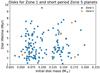 |
Fig. 1 Range of disk initial masses and lifetimes for the planet sub-population from APC used in this work. |
2.4 Comparing disk mass distribution to known systems
In Fig. 2 we compare the mass range of our protoplanetary disk model at four times through its evolution (0, 2, 4, 6 Myr) against the inferred masses of young (class 0/I) and intermediate (class II) aged systems. The young systems are from Tychoniec et al. (2018), while the intermediate aged systems are taken from Ansdell et al. (2016). For the class II systems we took the published dust mass and multiplied by the standard interstellar medium (ISM) value of the gas-to-dust ratio (100). This is in line with the assumption of Tychoniec et al. (2018) and ignores the possible discrepancy between observed CO fluxes and the total disk mass (Favre et al. 2013; Ansdell et al. 2016; Bosman et al. 2018b; Krijt et al. 2018; Schwarz et al. 2018, 2019; Booth et al. 2019).
In comparing to observations we see that the initial mass range (green) that we use is much less broad than is seen in the young population of systems seen by Tychoniec et al. (2018) (light blue). This includes primarily class 0/I objects with less gas mass than is included in our population. While we are naturally biased towards forming giant planets this discrepancy suggests that the lower mass systems seen in the observations may not lead to the formation of hot Jupiters and close-in Zone 5 planets.
As our models evolve through 2–4 Myr we find that our distribution overlaps with the higher mass end of the Ansdell et al. (2016) population of class II disks. Since planet formation via planetesimal accretion is generally slow (see for ex. Bitsch et al. 2015)we require larger mass disks to build Jupiter-mass objects within the lifetime of the disks. Hence based on the planetesimal paradigm, these lower mass disks do not generate large planets within the lifetime of the disk.
At the latest (6 Myr) stages our mass distribution begins to spread owing to differences in the photo-evaporation timescale tdep in Eq. (A.19). We still remain mostly at the large end of the observed mass distribution. This result is likely the result of our aforementioned bias towards the most massive disks.
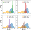 |
Fig. 2 Comparison of distribution of disk masses in our population of Zone 1 planets, evolved using the model presented in Sect. A.1. We show the mass of each of the disk models at its initial time, 2, 4, and 6 Myr into their evolution, even if the disk lifetime for any particular disk model is shorter than those times. We compare to the disk masses measured in a population of class 0/I from Tychoniec et al. (2018) and to a population of class II objects from Ansdell et al. (2016). |
3 Methods: disk astrochemistry
3.1 Volatile chemistry
As the temperature and density structure of the disk evolves over its lifetime, so do the molecular abundances of volatiles in the gas and ice. This is different from the refractory component of the disk, locked up in dust grains that remain (mostly) chemically neutral (but see below). As in our previous work (Cridland et al. 2016, 2017a), we used the Michigan chemical code (Fogel et al. 2011; Bethell & Bergin 2011; Cleeves et al. 2014) to compute the chemical kinetics of the gas and ice.
The Michigan chemical code computes the chemical kinetics of the gas and icy dust grains. The chemical network is predominantly in the gas phase, driven mostly by ions produced by cosmic-ray ionization and interactions with the high energy radiation fields described in Sect. A.3. Along with the ion and neutral gas-phase reactions there are a set of dust grain surface reactions that involve the freeze-out and desorption of volatiles and the production of H2O and H2 on the dust grain. The chemical network is based on the Ohio State University (OSU) gas-phase network (Smith et al. 2004) and includes additions made by Fogel et al. (2011) to include photo-dissociation, CO and H2 self-shielding, and non-thermal cosmic-ray ionization of H2 and helium.
As discussed above, we computed the growth and radial drift of the dust grains. The primary impact of the dust grain evolution changes the average size of the dust grains available for the freeze-out of volatiles. As the dust grains grow and radially drift in, the average surface area of the dust grains is reduced, which slows the volatile freeze-out in the outer disk. However unlike Booth & Ilee (2019) we did not couple the chemistry and dust evolution to account for the radial drift of icy volatiles. While this dynamical evolution was shown to may have an important impact on the local C/O of the gas and dust (Booth & Ilee 2019, but also see Krijt et al. 2016; Booth et al. 2017; Bosman et al. 2018a), it remains to be seen what impact this evolution has when coupled to the dynamic nature of planet formation (i.e. planetary migration also radially evolves the growing planet). We thus leave the implication of radially drifting dust on the local gas C/O to future work, and instead focus on the impact that smoothly varying the average size of the dust grains has on chemical processes such as volatile freeze-out and desorption (see Cridland et al. 2017a).
Previously, we accounted for any change in the molecular abundance of the gas in the disk by selecting many hundred snapshots of the gas temperature and density evolution of the disk and then computed the chemical kinetics for 1 Myr on each of the snapshots (Cridland et al. 2017a). The molecular abundance was initialized at the same abundance for each snapshot, and the chemical kinetics are computed for long enough to insure that the chemical system had run to a steady state. As a result the source of any chemical change is attributed to differences in the gas or dust properties between different snapshots.
Running the Michigan code in this “passive disk” method meant that running the chemical evolution over the lifetime of the disk was slow and spending roughly two to three months on a single astrochemical disk model meant that only a few disk models could be run at a time. Hence building a large population of models to test planet formation was not possible in any meaningful time frame.
A second side effect of the passive disk method was that by beginning each snapshot with the same initial state, we erased any evolution that had built upin previous snapshots. While we confirmed that differences that arose from initializing a snapshot with the results of the previous snapshot were small, these snapshots could build up as we ran hundreds of snapshots. Owing to the complexity of these large chemical systems, a more natural approach would be to allow the chemistry to evolve simultaneously with the gas and dust properties (temperature and density).
For this and subsequent work, we improved on the original Michigan code by allowing the underlying disk model (gas/dust temperature and density) to evolve along with the chemistry. To be clear, there is no back reaction between thechemistry and gas properties. The disk evolution is pre-computed using the methods described in Appendix A, which are then fed into the chemical code. We generated snapshots of the gas temperatureand density, which cover the entire evolution of the disk. These snapshots are temporally spaced by 104 yr, which sets the length of time over which the disk properties remain constant (see Fig. 3). Keeping the disk properties constant in this way supports the other disk properties (dust distribution, high energy radiation field) that are also pre-computed and are too computationally expensive to change continually.
In Fig. 3 we show an example of how the temperature and density structures evolve with time. Between time steps the physical properties of the disk remain constant, while the chemistry evolves. Then after the time step elapses the physical properties are changed and the chemistry continues. For comparison we note the evolution of water ice at 10 AU, which shows only minimal changes over the short time frame shown.
In Table 2 we show the initial molecular abundances used in the astrochemical simulations, we additionally note the C/O and C/N in the gas disk. The individual elemental ratios (excluding refractories) are C/H ~ 1.0 × 10⁻⁴, O/H ~ 2.5 × 10⁻⁴, and N/H ~ 2.45 × 10⁻⁵.
In Fig. 4 we compare the radial distribution of molecular abundances (along the mid-plane of the disk) for a few abundant species, which are computed by both the passive disk method (dashed lines) and the evolving disk method (solid line) at a time of 1 Myr. We find only minimal difference in the chemical abundances in the inner (r < 4 AU) disk, while farther out we begin to see a difference in the computed abundances. In particular we see a build-up of frozen CO2 and O2 in the outer disk.
The production of these molecules occurs (in our model) in the gas phase through a reaction of CO and the OH radical (for CO2) and elemental O with OH (for O2). In both cases the OH radical is required, which can be produced by the dissociation of H2 O, which explains the reduction of H2 O abundance in the same part of the disk in which CO2 and O2 become more abundant. This dissociation is driven by cosmic-ray induced UV photons and is quite slow (assuming the typical cosmic-ray ionization rate of ~10−17 s−1), requiring timescales of the order of a Myr to reach the reduction we see in the figure (see Eistrup et al. 2016 for t > 1 Myr of evolution). Hence by continually resetting the water abundances in each snapshot (as in the passive disk method), we are restricting these reaction pathways. Regardless, this resetting has little impact on our previous results, since every modelled planet accreted gas either near or within the water ice line within 2 AU at 1 Myr.
We notethat in our model the carbon budget in the outer regions of the disk is dominated by CO. This is because in our chemical model we do not include dust grain surface reactions such as the hydrogenation of CO ice to produce methanol (Drozdovskaya et al. 2014; Walsh et al. 2014; Eistrup et al. 2018). Since planet formation occurs far inwards of the CO ice line, omitting these reactions should not greatly impact the chemical compositions of our forming planets.
In Fig. 5 we show C/O in one of the disk models that we use in our population. The evolution of C/O is simpler than was shown in Cridland et al. (2019a) because we have ignored, for simplicity, the majority of gas-grain chemical reactions which are included in Eistrup et al. (2018). Similarly we see less evolution in the C/O of the ice species, which stays low over nearly all radii and time. An exception to this is in the inner disk at late times where the production and freeze-out of hydrocarbons eventually occurs, producing a low abundance of carbon species on the icy grains. Since the oxygen abundance of the ice is already small at these radii, the low abundance of these frozen carbon species result in these high C/O.
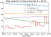 |
Fig. 3 Example of how physical properties of disk evolve between 0.5 and 0.7 Myr at a radius of 10 AU. The gas temperature, abundance of water ice, and UV flux are measured at the disk mid-plane. The gas temperature and density, dust density, and flux high energy radiation stay constant during a single time step. These values are then adjusted to a new value at the end of the timestep before the chemical evolution moves onwards in time. |
Initial abundances relative to the number of H atoms.
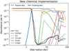 |
Fig. 4 Mid-plane distribution of primary carbon and oxygen bearing volatile molecules as computed by the original Michigan chemical code (passive disk) and our modified version (evolving disk). The label “(gr)” denotes molecules that are frozen on the dust grains. Each model is run up to 1 Myr, however in the evolving model the disk temperature and gas surface density evolves with time. |
3.2 Refractory carbon erosion
As was alluded to earlier, the majority of the refractory component of the disk, i.e. the dust and larger solid bodies, does not undergo significant chemical change over the lifetime of the disk. An exception occurs in the inner few astronomical units and has come to be known as refractory carbon erosion (called “depletion” in these works: Bergin et al. 2015; Anderson et al. 2017; Gail & Trieloff 2017; Klarmann et al. 2018; Cridland et al. 2019a). To avoid confusion we denote these processes as “erosion” since depletion is an astrochemical term generally connected to a reduction in gas-phase volatile abundances due to their incorporation into the dust grains; in this section we describe the opposite effect.
In the solar system the Earth shows a reduction in the bulk carbon relative to silicon of about three orders of magnitude relative to the ISM, while belt asteroids show a range of erosion between one and two orders of magnitude (Bergin et al. 2015). This observation encouraged Mordasini et al. (2016) to suggest a universality to this refractory carbon erosion and they have included this in their planet formation models.
More recently, Cridland et al. (2019a) include the chemical impact of carbon refractory erosion on the accretion of carbon in their formation model, but also include the excess gaseous carbon that would be released by the physical or chemical process responsible for the eroded carbon. A main result of their work is to show that this extra source of gaseous carbon in the inner disk could drive the C/O of hot-Jupiter atmospheres as high as ~2.5 times their value when the carbon excess is ignored.
We follow the same methods as in Cridland et al. (2019a). First they derive a functional form to describe the refractory carbon-to-silicon ratio (C/Si) in the disk based on Fig. 2 of Mordasini et al. (2016) as follows:
 (2)
(2)
where c ~ 5.2 is needed to connect the inner (<1 AU) disk to the outer (>5 AU) disk and rAU is the orbital radius in astronomical units.
In the ISM, Mishra & Li (2015) report Si/HISM = 40.7 ppm, which when combined with C/SiISM = 6 (Bergin et al. 2015) results in a refractory carbon abundances of C/HISM = 2.44 × 10⁻⁴. With that in mind the excess gaseous carbon in the disk would be
 (3)
(3)
A final level of complexity comes from the source of the refractory carbon erosion. This source is still not well understood and is complicated by the vertical mixing of the dust grains (Anderson et al. 2017) as well as their radial drift (Klarmann et al. 2018). We made the same simplification as in Cridland et al. (2019a) by requiring that the source of the excess carbon was either an ongoing process such as oxidation or photo-dissociation (as in Anderson et al. 2017) or was the result of a thermal event early in the disk lifetime that released the carbon from the grains (Bergin et al. 2015; Gail & Trieloff 2017). We differentiate these two models as “ongoing” and “reset”, respectively.
In the case of the reset model, the excess carbon would be released very early in the life of the disk and hence would advect towards the host star with the bulk of the gas. In the case of the ongoing model, the same advection would occur, but since the dust radially drifts into the erosion region and is processed, the excess carbon is replenished. Functionally the reset model has the form
 (4)
(4)
where vadv = 6.32 AU Myr−1 is the net advection speed of the bulk gas taken from Bosman et al. (2018a) for a disk with α =0.001. In the case of the ongoing model we set vadv = 0.
In our chemical models we do not include the excess carbon during the chemical kinetics simulation. Instead we simply accrete C/Hexc into the planetary atmosphere on top of the elemental carbon that is naturally available from the disk gas (see Table 2). Our assumption is that the excess carbon would remain primarily in the gas phase, producing CO (at the expense of H2 O), HCN, or CH4. However within 5 AU, Wei et al. (2019) show that long chain hydrocarbons can reform on the ice mantle with an abundance of approximately 1% of the total carbon elemental abundances. While we neglect the chemical impact of the carbon-excess in this work, we will account for the effect on atmospheric C/O by grain surface chemical reactions in future work.
The primary refractory source of oxygen is stored in silicates with SiO3 and SiO4 functional groups. To compute the elemental abundance of oxygen we followed Mordasini et al. (2016), who assume a refractory mass ratio of 2:4:3 for carbon, silicates, and iron respectively. This assumption leads to a refractory abundance O/Href = 1.75 × 10⁻⁴.
Before continuing, we note that the above physical processes describing the erosion of refractory carbon is separate from the ongoing discussion regarding depleted gaseous CO in the cold outer disk (r > 10 AU) suggested in recent ALMA surveys (Favre et al. 2013; Kama et al. 2016; Miotello et al. 2016; Yu et al. 2017; Bergin & Williams 2017; Cleeves et al. 2018; Schwarz et al. 2018). The process that we describe in this work is concentrated in the inner 5 AU of the disk, which does not have an effect on the observable volatile carbon abundance in the gas of the outer disk. We ignore, however, the impact of radial delivery of carbon and oxygen carrying volatiles by drifting pebbles as reported by Booth et al. (2017), Bosman et al. (2018a), and Booth & Ilee (2019). Hence the physical processes that are depleting the volatile carbon abundance in the outer parts of the disk could increase the carbon abundance in the inner solar system. This connection is computationally expensive to include in our model, and hence we leave its impact to further work.
 |
Fig. 5 Carbon to oxygen ratio (C/O) of gas and dust (ice and refractories) for a disk model in our population. The gas disk has a higher C/O than unity for ~ 0.5 Myr until the disk has cooled slightly. The ice is almost exclusively oxygen rich, apart from a region of the inner disk at late times caused by the slow production and freeze-out of long chain hydrocarbons. We included the excess carbon from the reset model, which eventually disappears after nearly 0.8 Myr. The solids in the region of the disk in which the carbonaceous dust is eroded is always oxygen rich, since the silicates remain in the dust grain while the carbon is removed. C/O changes most at the ice lines of the disk, particularly the water ice line between 2 and 3 AU. The CO ice line is located outside of 60 AU, and hence does not show up in the figure. |
3.3 Accounting for the accretion of ices and refractories
As is discussed in Cridland et al. (2019a) we assume that no refractory carbon or oxygen that accretes into the core is incorporated into the atmosphere, by either erosion or outgassing. We assume that once the gas envelope is sufficiently massive (more than 3 M⊕, see below), planetesimals can begin to deliver ices and refractories.
Mordasini et al. (2015) compute the survivability of planetesimals as they pass through a planetary atmosphere. This calculation is complicated and involves self-consistent models of planet formation, atmospheric structure, and thermal processing of the incoming planetesimals.
We strive to capture the essence of these more complicated models by assuming that below an atmospheric mass of 3 M⊕ the refractory component of the planetesimal remains intact through the atmosphere and is incorporated into the core. This cut-off is based on the calculation done by Mordasini et al. (2015) and represents a minimum atmospheric mass above which planetesimals of all sizes are evaporated within the atmosphere. During their trip through the atmosphere, these planetesimals are heated as they pass through the gas releasing any frozen volatiles into the atmosphere. We assume that a planetesimal releases its entire volatile component upon entering an exoplanetary atmosphere (of any mass).
When the mass of the atmosphere grows above a mass of 3 M⊕, planetesimals are completely evaporated in the atmosphere, releasing their volatiles and refractories into the gas. We assume efficient mixing such that these planetesimals incorporate their refractory carbon and oxygen into the bulk C/O.
4 Results: chemical population synthesis
4.1 Population of planets
In Fig. 6 we show the final mass and orbital radius of the planets in the population from APC. A benefit of this population is that there is generally little bias, showing no structure in this parameter space. We find that the lower mass range of the population are generated in disks with lower lifetimes. This is caused by the growth of the planet being cut off by the final evaporation of the disk gas (also see Alessi & Pudritz 2018).
On the other hand, the three lowest mass planets form in disks with the longest lifetime. This is caused by the fact that long-lived disks tended to evolve slower (by construction, see Eq. (A.19) with tdep = tlife). These light planetsbegan at far radii in the dead zone in the most massive disks, and needed the full lifetime of the disk to migrate to their ending position. While massive, their natal disks tended to have lower metallicity, and hence their cores formation was less efficient. The location of the dead zone of the disk is dominated by the surface density of dust and gas density which set the ionization level of the disk gas.
Planets with the largest mass and smallest orbital radii also occur in the longest lived disks, since they required the longest time to migrate inwards. These massive planets formed in heavier disks (and/or high metallicity disks) where they could grow more quickly then the lowest mass planets. These planets were all generated by protoplanets trapped at the dead zone (and one trapped at the heat transition). In what follows we compute the atmospheric C/O for this population of planets and search for any dependency on their planet formation history.
4.2 Ignoring solid accretion
In Fig. 7 we show the C/O for our population of planetary atmospheres. The vertical dashed line shows the bulk C/O of the disk gas. We find that the majority of planets result in a similar C/O as was initialized in the disk. This result is not surprising and has been seen in our previous work (Cridland et al. 2017a). The main reason for this is that these planets have migrated inwards of the water ice line before they accrete the majority of their gas. Inwards of the ice line there are no volatiles frozen onto the grains, hence C/O remains unaffected with respect to the initial ratio.
For planetary masses between 25 and 790 M⊕ we see our first deviation from the bulk C/O caused by the formation history of the planet. In this mass range C/O can get as high as ~ 1 because these planets have accreted their gas outwards of the water ice line. Planets with C/O > 0.4 grow in both the ice line and dead zone planet traps.
Planets in the dead zone trap have simply not migrated within the ice line before they begin accreting their gas. Hence the gas is more carbon rich because water is in its ice phase. In the case of the ice line planets, their formation is occurring embedded within the dead zone of their disk (at smaller radii than the dead zone trap), where the turbulent viscosity is much lower. As a result these planets easily open a gap even when they are only a few times the mass of the Earth (recall Eq. (B.7)). The planets enter into a stage of Type II migration much earlierthan other protoplanets of that size and lag behind the evolution of their ice line. This keeps these planets outwards of the water ice line of the disk where C/O is larger than 0.4. In total we find 33.5% of planets in our sample end up with larger C/O than the bulk disk gas.
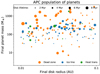 |
Fig. 6 Test population of hot Jupiters and close-in super-Earths taken from APC. This population covers a wide range of final radii and mass. We note whether the planet grew in the dead zone, water ice line, heat transition (heat trans), and lifetime of the disk in which the planets grew. |
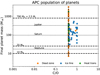 |
Fig. 7 Carbon-to-oxygen ratio for the population of planets assuming that gas accretion is the sole source of carbon and oxygen in the atmosphere. The vertical dashed line denotes the C/O of the gas disk, which the majority of planets mimic. |
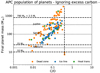 |
Fig. 8 Carbon-to-oxygen ratio for the case including solid accretion into the atmosphere, but ignore the excess carbon in the gas phase. As such, solid accretion predominately delivers oxygen-rich silicates and ices to the exoplanetary atmospheres. |
4.3 Including solid accretion
While gas accretion surely dominates the mass of Jupiter-mass planets, solid accretion can contribute a significant fraction of the carbon and oxygen to their atmosphere. This comes from the fact that in the gas, carbon and oxygen make up approximately 0.01% of the atoms or about 0.1% of the mass. Meanwhile the refractories are dominated by silicates (along with irons), and dust with ISM levels of carbon can be built up with a few tens of percent of carbon (by mass). Hence at least 100 times more gas than solids must be accreted in order for the same number of carbon or oxygen atoms to be delivered to the atmosphere. This requirement becomes difficult for even a Saturn-mass planet (M ~ 95 M⊕).
4.3.1 Ignoring the carbon excess model
We begin in Fig. 8 by assuming that the excess carbon discussed in Sect. 3.2 does not contribute to the carbon content of the gaseous disk. In this way we ignore the impact that the depleted refractory carbon can have on the carbon budget of the disk gas. This is equivalent to assuming that the excess carbon moves with the bulk gas at a rate much faster (at least two orders of magnitude) than is assumed in the reset model. As such the only extra element available for accretion in this situation is the oxygen that is incorporated in the ice (if the planet is growing outside the water ice line) and silicates.
Without the extra carbon, we find in Fig. 8 that all of the planets end with smaller C/O than in the case of gas accretion alone. An exception to this can be found in our two lightest planets (with M < 10 M⊕), which show no change in their C/O from the case of gas accretion alone. This arises because their atmosphere mass never exceeds 3 M⊕, which was the assumed cut-off above which planetesimals evaporate in the planetary atmosphere. Hence for these planets the incoming planetesimals reach the core of the planet, and only volatiles may contribute to the atmosphere; we note that ignore core erosion.
At slightly larger masses (10 M⊕ < M < 25 M⊕) the atmosphere has surpassed the 3 M⊕ cut-off and refractory sources of carbon or oxygen can contribute to the atmosphere. For these planets the incoming carbon and oxygen is dominated by refractory sources because the planet has not reached a large enough mass to undergo unstable gas accretion. As a result the ratio of gas and dust accretion timescales are close to one and the accretion of refractory oxygen is its dominant source.
As for these lower mass planets, for masses >25 M⊕ the combination of solid and gas accretion determines the final C/O. We see a spread in final C/O depending on where the planet begins its evolution. For a given mass range, planets that were trapped at the water ice line (blue) or began in traps near the ice line tend to have higher C/O than planets that formed farther out in the disk. The planets that formed in the dead zone (orange) and heat transition (green) farther out than the water ice line (see Fig. 9) grew in a part of the disk at which the surface density of solid material is reduced because of the radial drift of the dust (see for example Cridland et al. 2017b).
Since they start at further radii, the initial growth rate of planets at the dead zone and heat transition is slower than at the ice line (andin models in which the dead zone and heat transition begin near the water ice line). These planets take much longer to build a core that is capable of undergoing unstable gas accretion, which allows more time for solids to accrete into the atmosphere.Ice line planets accreted much faster than planets starting in the dead zone or heat transition and hence accreted less solids (by mass) than planets that underwent slower core formation. In this model we lose planets with C/O > 0.4, since these planets also accrete (oxygen-rich) ices along with the silicates in the incoming planetesimals.
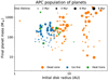 |
Fig. 9 Starting radii of the planets in our population. Generally the planets trapped at the ice line begin within a small range of radii since the location of the ice line is only weakly dependent on initial disk mass. We note that planets that start between 10 and 20 AU do not end their evolution as hot-Jupiter or close-in super-Earths, hence the deficit of points. |
4.3.2 Including the carbon excess models
In Figs. 10a and b we show the effect on the population from the two chemical models presented in Cridland et al. (2019a). In the reset model (Fig. 10a) the excess carbon is allowed to advect with the bulk gas motion of the disk, quickly (in about ~0.8 Myr) accreting into the host star. Because of its rapid evolution, most of the planets are unaffected when moving from the model shown in Figs. 8–10a, however there are a few planets that evolve rapidly enough to be coincident with the region of the disk that has excess gaseous carbon when the planet undergoes gas accretion.
For an example of this, two Jupiter-mass planets with C/O < 0.1 are shifted to C/O ~ 0.2 in the reset model of carbon excess. This is because these planets evolve fast enough that they accrete their gas in a region of the disk at an early enough time that the excess carbon has not disappeared.
Finally in Fig. 10b we show the results of the ongoing model. The excess carbon is constantly replenished by the radial drift of dust grains and hence the gaseous excess carbon remains high in the inner disk. When comparing to the model in Fig. 10a we find that all of the planets have shifted to the right (i.e. towards being more carbon rich).
This shift does return many of the higher mass (M > 100 M⊕) planets to be more carbon rich (C/O > 0.4), however none of these planets result in atmospheres with C/O > 1. The lowest mass planets (M < 10 M⊕) also show carbon-rich atmospheres since they are not chemically affected by solid accretion, instead feeding exclusively on the carbon-rich gas present in this model.
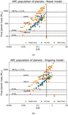 |
Fig. 10 Same as figure Fig. 8 but for the reset model (panel a) of carbon excess with a constant net advection speed of 6.32 AU Myr−1 as prescribed by hydrodynamic disk models. As such, some planets reach a region of the disk at which the excess carbon remains in the gas phase in time to incorporate it into its atmosphere. For the ongoing model (panel b) the net flux of the excess carbon is zero, which keeps a high carbon abundance. As such most of the planets reach a region of the disk at which the carbon is enhanced owing to the ongoing processing of dust grains. |
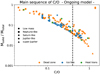 |
Fig. 11 Main sequence of C/O for the planet in our population. Over a wide range of masses we find that lower C/O is caused by the total mass of planet coming predominantly from solid (refractory) sources. The exception comes from the low mass planets (M < 10 M⊕), which are not chemically affected by the accretion of planetesimals. |
4.3.3 C/O main sequence
In Fig. 11 we generalize these results into a main sequence of C/O for the planets in this population. This sequence is relevant for planets that surpassthe 3 M⊕ atmospheric mass limit to evaporate planetesimals in the atmosphere fully. We show only the main sequence for the ongoing model since only minor differences (other than a horizontal shift) arise from changing the carbon refractory model. In the figure we differentiate between low mass (M < 10 M⊕), Neptune-like (10 M⊕ < M < 40 M⊕), Saturn-like (40 M⊕ < M < 200 M⊕), Jupiter-like (200 M⊕ < M < 790 M⊕), and super-Jupiter (790 M⊕ < M) planets. We see little spread off the main sequence from different mass ranges, except the low mass planets, which are far off the trend for their solid mass fraction. As was already mentioned, this comes from the fact that these planets never have heavy enough atmospheres to evaporate incoming planetesimals.
For illustrative purposes, Jupiter has a solid-to-total mass ratio of ≲ 0.07 (Wahl et al. 2017) which, according to Fig. 11 results in a range of possible C/O between 0.2 and 0.6. Given that Jupiter’s atmosphere is enhanced in carbon by a factor of 4 above the solar value (Atreya et al. 2016), then this range of C/O implies that its expected oxygen abundance should be between 10.6 and 3.6 times the solar oxygen abundance. Of course, these simple calculations assume that Jupiter formed in a similar region as the hot Jupiters in our model, near the water ice line. This requirement is consistent with the Grand Tack model of the formation of Jupiter and inner solar system, which starts Jupiter’s outward migration inwards of the water ice line.
In summary, the figure makes an important new point. For planets along the main sequence that gain enough atmosphere mass to evaporate planetesimals, the smaller the contribution that solids have on the total mass of the planet, the higher their atmospheric C/O. The total mass contribution by solid accretion could additionally be interpreted as the atmosphere metallicity, which we explore below.
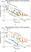 |
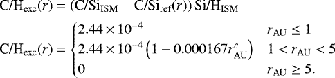
Fig. 12 Mass-metallicity relation for two tracers O/H (panel a) and Si/H (panel b). We similarly show the metallicity for the solar system giants (inferred by methane abundance and taken from Kreidberg et al. 2014), WASP-43 b (Kreidberg et al. 2014), GJ 436 b (Morley et al. 2017), and HAT-P-26 b (MacDonald & Madhusudhan 2019) from their water abundance. We find that our Neptune-mass planets are consistent with the metallicity of HAT-P-26 b, but not with Uranus or Neptune, suggesting the formation location could be important to O/H. The Si/H spread in metallicity for a given planet mass is caused by the accretion of solids. In this case our Neptune-mass planets are consistent with the inferred metallicity of Uranus and Neptune. |
4.4 Mass-metallicity relation
In our solar system, high mass planets tend to have lower metallicity (Atreya et al. 2016), which is often attributed to the amount of solid material that was accreted during their formation (relative to the gas accreted). More generally, this trend has been inferred in the exoplanet population (see for example Miller & Fortney 2011; Thorngren et al. 2016; Thorngren & Fortney 2019) as derived from interior structure modelling.
In Figs. 12a and b we show the mass-metallicity relation for our population of planets given two methods of inferring themetallicity: oxygen-to-hydrogen (O/H) and silicon-to-hydrogen ratio (Si/H). We compare our population of planets to the solar system giants and three exoplanets. The range of metallicity for the solar system giants (inferred by methane abundances) and WASP-43 b (inferred from water abundance) were taken from Kreidberg et al. (2014). The metallicity of the hot Neptunes GJ 436 b and HAT-P-26 b are inferred by their water abundance by Morley et al. (2017) and MacDonald & Madhusudhan (2019), respectively. For a given mass, lower metallicity planets generally came from the water ice line, accreting very quickly, which limited the amount of solids that could be accreted into the atmosphere.
In Fig. 12a we show the atmospheric metallicity (as inferred by O/H) for our population of planets. In this way we can best compare to the exoplanet observations, since their metallicity was inferred by an abundant oxygen carrier. We see that HAT-P-26 band WASP-43 b agree well with O/H of their respective mass range. In the Neptune-mass range we under-predict the O/H metallicity of Uranus and Neptune, which can be explained by a lack of icy planetesimal accretion in HAT-P-26 b; the opposite is true for Uranus and Neptune. This suggests that the Neptune-like planet HAT-P-26 b likely formed inwards of its water ice line of the disk.
For GJ 436 b we see that we have under-predicted its metallicity by almost two orders of magnitude. Since it is known to orbit very close to its host star this can be explained by a significant amount of atmospheric evaporation.
In Fig. 12b we compare the metallicity of each of our planets as inferred by Si/H to the metallicity of the solar system giants and three exoplanets. Once again we see that the relation between planet mass and metallicity inferred by Kreidberg et al. (2014) agrees well with the general trend in the figure. The large spread is caused by the amount of solid accretion that the growing planets have experienced. The spread is larger than we find in Fig. 12a because the source of silicon is strictly from planetesimal accretion, while oxygen can also be accreted directly from the gas.
Generally we find that the mass-metallicity relation is most determined by the fraction of solid mass accretion relative to the total mass of the planet. However different tracers of metallicity can be subject to factors other than the total mass accretion. The O/H can be most sensitive to variations due to the position of the disk relative to the water ice line, as well as the physical history of the atmosphere after formation. In particular, Neptune-mass planets are most sensitive to their formation history because a majority of their oxygen can come from refractory sources.
We note that along with our C/O main sequence introduced in the previous section, the mass-metallicity implies an anti-correlation between planet metallicity and atmospheric C/O, as discussed by Madhusudhan et al. (2014, 2017) and Espinoza et al. (2017). In our work this anti-correlation is a direct result of the relative importance that solid accretion has on the total mass of the planet and the quantity of solids that can be delivered into the planetary atmosphere. These solids are oxygen-rich (relative to carbon) as proposed by Öberg et al. (2011) when we include refractory carbon erosion, hence Neptune-like planets that are dominated by solid accretion are found to have remarkably low C/O.
5 Discussion: observed C/O and formation history
We would like to answer whether a measured C/O can give any insight into the formation history of a planet. As we have seen, this interpretation is complicated by the treatment of solid accretion and the excess carbon expected to be generated from refractory sources.
5.1 General trends
Generally we see that low mass (M < 10 M⊕) planets are not affected by solid accretion because their atmosphere are not heavy enough to evaporate incoming planetesimals. Additionally our model suggests that these close-in, low mass planets have accreted their gas within the water ice line. These planets could give us a secondary method of probing refractory carbon erosion. However due to their size they are difficult to characterize and probing them efficiently will likely require observations by the James Webb Space Telescope (JWST). A second possibility for these low mass planets exists: they grow outside of the ice line and are dynamically scattered into the inner solar system after the evaporation of the disk gas. Hence the presence of an unknown companion may be inferred. Only follow-up observations will confirm this along with details of carbon refractory erosion, but new results would nevertheless add to our ever growing knowledge of planet formation.
At slightly higher mass ranges (10 M⊕ < M < 25 M⊕ ; Fig. 11) the accretion of solids dominates the delivery of carbon and oxygen. In the case of close-in planets, our models predict that this mass range is highly oxygen rich because of the high percentage of mass that is composed of silicates. For planets in much longer orbits than investigated in this work (as in Neptune), we might expect much higher C/O ratios owing to the accretion of more carbon-rich planetesimals; we also might find enrichments of both O/H and C/H, as observed for Neptune (Atreya et al. 2016). Even in the case in which excess gaseous carbon is included (Fig. 10) these planets remain at very low C/O. Hence we expect very strong water emission/absorption features to be present in these types of close-in planets. Because of their dependence on solid accretion history, these Neptune-like planets could act as a useful tracer of alternative accretion models such as pebble accretion (Johansen et al. 2007; Ormel & Klahr 2010; Bitsch et al. 2015).
For Saturn- and Jupiter-like planets (25 M⊕ < sM < 790 M⊕; Fig. 11) we find a larger deviation in the bulk C/O, which depends on where the planet began accreting. For planets beginning near the water ice line (trapped in any of the three traps), their bulk atmospheric C/O stays within an order of magnitude of the fiducial gas disk C/O. However this is heavily dependent on the excess carbon model.
Planets that began their evolution outside the water ice line generally have accretion timescales that are long as a result of lower dust (and hence planetesimal) column density, and hence can accrete a high percentage of their carbon and oxygen from refractory sources. Hence sub-Saturn mass planets (M < 100M⊕) should have sub-stellar C/O while larger planets may accrete enough gaseous carbon to have stellar-like (or larger) C/O.
For the largest planets (M > 790 M⊕; Fig. 11) the effect of solid accretion results in only small scatter, since the majority of their mass comes directly from gas accretion. The most massive planets have the highest C/O since their gas-to-solid accretion is the highest. They are very dependent on which model is controlling the distribution of the carbon excess. In the cases in which the excess carbon from the refractories disappears because this excess flows in with the bulk disk gas (i.e. the reset model), all of the highest mass planets have sub-stellar C/O.
To have atmospheres with C/Oplanet > C/Ostar we require an ongoing process producing excess carbon in the gas phase that is accreted by these growing planets. The shift to the right between Figs. 10a and b (also see Fig. 13) depend on what extent the refractory carbon is depleted from the grains in the region in which the planet formed. Hence in the case that excess carbon survives for the full lifetime of the disk, then all of the highest mass planets have stellar-like or super-stellar C/O, some even approaching C/O ~ 1. This suggests that if the detection of high C/O among massive planets continues to be common, the ongoing model might be the best description of the excess carbon distribution.
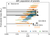 |
Fig. 13 Comparing the observed atmospheric C/O (black) shown in Table 3 to our population of planets. Each line segment represents the shift in C/O between the carbon excess models shown in Figs. 10a and b for each synthetic planet. Additionally we include an increase in C/O in Neptune GJ 436 b-like planets caused by a rain of silicates (dashed line; see the text). |
5.2 Comparing to observations
As we implied earlier, comparing our synthetic chemical population of planets to the observed population is necessary to understand the properties of planet formation.
In Fig. 13 we show a comparison between our synthetic population of planets to a small set of characterized planetary atmospheres. The individual planets along with their values, ranges, and references are found in Table 3. The coloured line segments note the shift in C/O caused by the two carbon excess models shown in Figs. 10a and b. The points show a specific C/O outlined by observation, while the black line segments denote possible ranges of observed planets determined through retrieval methods.
Generally speaking these planets all lie above C/O = 0.4, placing them in the population of planets that begin their growth either trapped at the water ice line, or at a planet trap that originated near the ice line. This tendency of beginning their evolution near the water ice line is consistent with the works of Dra̧żkowska & Alibert (2017), which suggest that a dust pile up at the water ice line due to radial drift leads to efficient planetesimal formation which should then lead to more rapid growth of the first planetary cores.
A particular oddity appears to be in the hot-Neptune GJ 436 b (as reported by Madhusudhan & Seager 2011 and Morley et al. 2017), which appears near the bottom right part of Fig. 13. With its mass of ~ 22 M⊕, hot-Neptune GJ 436 b is in a mass regime that we attribute to predominately (very) low C/O because a high percentage of its accreted mass is from solid bodies. This could be a sign that the excess carbon from refractory carbon erosion is not a universal process, since a system that has not undergone refractory carbon erosion would produce carbon-rich Neptune-mass planets at small radii from its carbon-rich (i.e. ISM-like) refractory component.
This discrepancy can also be explained by chemical processing of the gas within the atmosphere over the following billions of years after formation. With the silicon that is delivered to the atmosphere, some of the oxygen can be locked back into refractory material that precipitates out of the upper layers of the atmosphere. This would increase the observed C/O as described in Helling et al. (2014), assuming that the carbon is not also captured in these refractory grains.
To that end we run a simple test of chemical equilibrium models at a range of temperatures (500–1500 K) and gas pressures (10−4 bar–0.1 bar) with the initial elemental abundances of H, C, O, N, and Si as computed by our planet formation model for the four planets with masses similar to that of GJ 436 b. We find that the observable C/O (i.e. in CO, CO2, CH4, and H2 O) increases by roughly a factor of 4.5 (across the range of pressure and temperatures used in this work) because some of the oxygen condenses out of the gas in silicates and (presumably) rains from the upper atmosphere or produces clouds.
In Fig. 13 we also show the shifted C/O for the four Neptune-mass planets by the factor of 4.5 from our chemical equilibrium model. Clearly the increased C/O shift these planets to the right of the figure, however not far enough to explain GJ 436 b. Hence chemical processing after the atmosphere has formed is insufficient to fully explain this planet.
A second planet with a similar mass is HAT-P-26 b, which has a recently reported C/O upper limit by MacDonald & Madhusudhan (2019) of 0.33. This is more consistent with our maximum allowed C/O from our formation model and equilibrium chemistry. MacDonald & Madhusudhan (2019) have also reported the detections of metal hydrides (TiH, CrH, and ScH) at lower (< 3.6σ) signal to noise. These gas-phase detections at the moderate (~500 K) temperature of HAT-P-26 b suggest that non-equilibrium processes must be dominating over pure chemistry (as assumed in our chemical equilibrium model). The complexity of the chemical and physical processing of atmospheres in this mass range is intriguing, but we leave this to future work.
Currently most observed C/O (including upper limits) in exoplanetary atmospheres fall within an order of magnitude. This is partly caused by the fact that current observations do not cover a wavelength range in which the most abundant carbon carriers (CO, CO2) have strong spectral features. This will be greatly improved over the next decade with the launch of JWST and wide wavelength range of its instruments.
In summary the observed atmospheric C/O all fall within an order of magnitude of each other, regardless of planetary mass. This suggests that the amount of post-formation chemical processing in the atmosphere will be more pronounced for the lower mass planets, since their fraction of oxygen in the atmosphere coming from refractory sources is higher. As such high mass planets do not undergo as much chemical processing as discussed above since their Si/O is lower. Additionally these Neptune-like planets could be more sensitive to chemical interactions between the atmosphere and core, which we do not account for in this model.
Observed C/O and/or inferred ranges of possible C/O for planets that orbit at < 0.1 AU.
5.3 Comparison with previous theoretical work
As previously mentioned, other theoretical studies have struggled to produce high super-solar C/O owing to simplified chemical models (Mousis et al. 2011; Ali-Dib 2017) or depleted gas disks caused by inwards accreting bulk gas (Thiabaud et al. 2015; Mordasini et al. 2016). In these cases the accretion of solids leads to very low C/O predominately because of oxygen-rich building blocks (both planetesimals and pebbles). Because of this tendency, it has been difficult to reconcile some recent observations that suggest high C/O.
In the case of Ali-Dib (2017), a high C/O was achieved by assuming a large core erosion efficiency, which incorporated the carbon and oxygen from the metal-rich core into the atmosphere. Their refractory component incorporated an assumed quantity of 80 and 50% of the total carbon and oxygen, respectively. In our model, refractory carbon and oxygen represent 70 and 40%, respectively,resulting in a higher refractory C/O (=1.4) than their model (=0.88). In this case, the impact of core erosion could be more strong than is suggested in Ali-Dib (2017), however numerical simulations have shown that the mixing efficiency from the core to the atmosphere can be more inefficient than previously thought (Moll et al. 2017).
Thiabaud et al. (2015) and Mordasini et al. (2016) deplete their volatile carbon and oxygen from the gas by accreting it into the host star within the first Myr. The gas that replaces the accreted gas comes from farther out in the disk where the volatiles have frozen out. While this gas moves inwards, the frozen volatiles would similarly move inwards, where they would also lose their ices to desorption (Bosman et al. 2018a; Booth & Ilee 2019). Hence the volatile component of the disk is maintained over a longer timescale where it can be available for accretion onto growing planets. Similarly, extra carbon and oxygen can be delivered just within the ice lines of various volatiles; this potentially offers a separate pathway towards enhance the carbon and oxygen component of atmospheres (Booth & Ilee 2019).
Moreover, the studies which include the impact of refractory carbon erosion in the composition of the refractories have not included enhanced carbon in the gas that would result. In this way their disks tended to be very oxygen rich in the inner solar system, causing the resulting exoplanetary atmospheres to be similarly oxygen rich. In this work, we used the excess carbon models of Cridland et al. (2019a) to account for the abundance and evolution of the carbon released by the erosion of refractory carbon. In this way the gas can become quite carbon rich (recall Fig. 5) in the region of the disk where the majority of planets accrete their gas.
In our work we can reproduce high C/O in planets with high mass (Mplnt > 100 M⊕) only if refractory carbon is continuously eroded throughout the lifetime of the disk. If this is not the case, our models revert to previous studies which predict solar or sub-solar C/O. We did not consider the erosion of the planetary core in this work, however its role in setting the final atmospheric abundances could be important. Similar to the aforementioned studies we do not produce C/O > 1, except for planets with mass <10 M⊕ in the ongoing carbon excess model. This result is simply because the chemical composition of these atmospheres is not impacted by the accretion of planetesimals, and hence only impacted by gas accretion.
5.4 Caveats
In principle, there are carbon-rich planetesimals outside of the 5 AU radius, which we set as the radial extent of the carbon erosion region of the protoplanetary disk. Indeed comets that originate from orbits farther out than Jupiter show ISM levels of C/Si in our own solar system (Bergin et al. 2015). However every planet in our population begins accreting gas inside of 5 AU, hence any planetesimal that it can accrete (according to our model) is carbon poor. This ignores two possible complications to our model. Firstly the core of the planetesimal can be built outside of the 5 AU extent of the carbon erosion region. The carbon-rich core could release its carbon into the atmosphere by out gassing or core erosion as in Madhusudhan et al. (2019). This effect is a complicated physical problem, and hence we ignored its contribution to the carbon content completely. However this effect could be important for Neptune-like planets, in which the core makes up a higher percentage of the total planetary mass.
Second we ignored the possible effect of dynamical mixing of carbon-rich planetesimals from the outer disk into the inner disk, which could potentially deliver extra carbon to growing planets in the inner disk (r < 5 AU). This process apparently did not happen in our solar system (since carbon erosion can be seen today) and could be caused by the presence of Jupiter acting as a guard to the inflow of carbon-rich solids. Systems that lack a Jupiter-like planet at radii outside the 5 AU erosion region could continue to have refractory carbon delivered to the inner disk, and if there is no ongoing process actively taking carbon away from the solids (as is assumed in the reset model) then extra refractory carbon would be available for accretion.
Finally, Jupiter should have acted as a barrier to inward drifting dust grains in our own solar system. As such it would have stopped the flow of incoming refractory carbon in the ongoing model. In a more general case, planetary systems that also contain a Jupiter-like planet at larger radii could see an ongoing-like model of refractory carbon erosion being suppressed. Given the importance of the ongoing model to explain the observed C/O of characterized exoplanetary atmospheres, more work is needed to understand the details involved in depleting the refractory carbon in inner planetary systems.
6 Conclusions
In this workwe have combined the method of planet population synthesis with the astrochemistry of protoplanetary disks to predict the atmospheric C/O in a population of hot-Jupiter and close-in super-Earth planets. For gas accretion alone we find that the majority of planetary atmospheres have C/O that match the elemental ratio of the gaseous protoplanetary disk. However for a small subset of planets we find C/O that exceed the protoplanetary disk gas because they accreted their gas outwards of the water ice line at which water has frozen out on the dust grains.
Going beyond simple gas accretion we include the chemical effect of accreting planetesimals into the growing planetary envelope. We simply parametrize detailed studies of planetesimal survival through an atmosphere and assume that if the gaseous envelope is below 3 M⊕ then the refractory material in the planetesimal reaches the core. Otherwise the planetesimal is completely destroyed in the atmosphere. In both cases, we assume that the volatile component of the planetesimal is delivered into the atmosphere.
The consequence of solid accretion on the amount of carbon and oxygen in the atmosphere depends on the fraction of accreted mass that comes from planetesimals and whether those planetesimals deliver their material into the atmosphere or to the core. The chemical make-up of these planetesimals includes the effect of refractory carbon erosion in our model, and hence within 5 AU the majority of refractories are oxygen rich. Broadly speaking our results show the following:
-
Low mass (M < 10 M⊕) planets do not accrete enough of an envelope to destroy planetesimals fully as they pass through the growing atmosphere. C/O is determined by gas accretion alone.
-
Neptune-mass (10 M⊕ < M < 25 M⊕) planets have enough of an envelope to evaporate incoming planetesimals before they reach the core. These planets accrete a high percentage of their carbon and oxygen from these refractory sources, and hence they are oxygen rich.
-
Saturn- and Jupiter-mass planets (25 M⊕ < M < 790 M⊕) show a wide range of atmospheric C/O partly because of the fraction of refractory sources that contribute to the carbon and oxygen. Additionally this mass range shows some deviation in at what point planets begin their evolution. Planets that start either in the water ice line, or near the water ice line (but in another trap), tend to have higher C/O than planets that begin at larger orbital radii.
-
Super-Jupiter-mass (M > 790 M⊕) planets show less of a tendency of starting their growth near the water ice line. These planets follow a similar trend as the Jupiter-mass planets which started their evolution outwards of the water ice line.
-
All planets above a mass of 10 M⊕ fall along a main sequence between C/O and the fraction of solid mass that make up the total mass. This main sequence applies for planets that have accreted enough of a proto-atmosphere that incoming planetesimals evaporate completely.
-
The mass-metallicity relation is explained well with the fraction of solid mass (relative to total mass) that is accreted into the atmosphere. However variations from formation history can be particularly important to the inferred metallicity of Neptune-mass planets if the inferred metallicity is from O/H.
We compared our results to the inferred C/O from a number of planets whose atmospheres have been chemically characterized and whose orbital radius is less than 0.1 AU. We find that
-
Observed hot-Jupiters are consistent with the higher range of C/O found in our synthetic planets. This tendency suggests that these planets begin their accretion near the water ice line of their respective disks.
-
Neptune-like planets GJ 436 b and HAT-P-26 b have much higher C/O (by about two orders of magnitude) than inferred by our model. We show that part of this discrepancy could be caused by chemical processing, which produces condensible materials which locks up oxygen and removes it from the gas in the upper atmosphere.
-
A discrepancy in low mass C/O could also suggest that refractory carbon erosion is not a universal process, and the two planets we included in this work were formed in a disk with carbon-rich refractories. This could similarly suggest that refractory carbon can reform on the grains, as proposed by Wei et al. (2019).
-
Additionally the discrepancy could be caused by the dynamical delivery of carbon-rich planetesimals from the outer part of the disk. This effect however, is beyond the scope of our work here.
We have shown that variation of the atmospheric C/O ratios of planetary atmospheres arise through a planet’s mass accretion alone. We see this variation even though we assume that the stellar C/O does not vary between stellar systems. However as shown by Brewer & Fischer (2016), higher metallicity stars tend (with scatter) to have higher C/O. This suggests that some scatter in atmosphericC/O comes from the difference in the initial elemental abundances of the stellar system. To what extent this effect increases the scatter above planet formation alone will be an interesting line of research that we will explore in a future paper. In conjunction with the next generation of telescopes and their impact on characterizing the chemistry of exoplanetary atmosphere, we will continue to use chemistry to learn about the underlying details of planet formation.
Acknowledgements
We thank the two anonymous referees whose advice was greatly appreciated, and improved the quality of the manuscript. Thank you to Paul Mollière and Arthur Bosman for their spirited discussions and use of Paul’s chemical equilibrium code. Astrochemistry in Leiden is supported by the European Union A-ERC grant 291141 CHEMPLAN, by The Netherlands Research School for Astronomy (NOVA), and by a Royal Netherlands Academy of Arts and Sciences (KNAW) professor prize. The work made use of the Shared Hierarchical Academic Research Computating Network (SHARCNET: www.sharcnet.ca) and Compute/Calcul Canada. R.E.P. is supported by an NSERC Discovery Grant. M.A. acknowledges funding from NSERC through the PGS-D Alexander Graham Bell scholarship.
Appendix A: Protoplanetary disk model
The important backbone to both planet formation and astrochemical studies is the protoplanetary disk model, which describes the distribution of the gas and dust. For the gas we use a modified version of the analytic disk model of Chambers (2009), while for the dust we use the two-population model of Birnstiel et al. (2012). These models are outlined below.
A.1 Gas model
The disk model of Chambers (2009) is a self-similar solution to the diffusion equation, assuming that gas accretes towards the host star at a constant rate of (Alibert et al. 2005)
 (A.1)
(A.1)
within a disk radius rswitch and away from the host star outside rswitch at the same rate to conserve angular momentum. The quantity Σg is the gas surface density and the viscosity (ν) is given by the standard α prescription (Shakura & Sunyaev 1973). With this prescription, the viscosity is ν = αcsH, where cs is the gas sound speed and H is the gas scale height. The source and size of the disk α, which parametrizes the angular momentum transport by either gas turbulence or magnetic winds, is not well constrained and is an ongoing topic of discussion (Bai & Stone 2013; Bai 2016, 2017; Tazzari et al. 2017; Najita & Bergin 2018; Pascucci et al. 2018; Wang et al. 2019; Milliner et al. 2019).
As was done in past work (see Cridland et al. 2017a; Alessi & Pudritz 2018), we assume that the disk α is a combination of both turbulence and disk winds: α = αturb + αwind such that it is a constant throughout the whole disk, where α = 0.001. In this way, we assume by construction that the gas turbulence and magnetic winds are working in tandem to maintain a constant accretion through the disk. Even when (for example) the gas is passing through a dead zone, where αturb drops (see below).
The gas is heated by two sources: the loss of gravitational energy as material accretes and the direct irradiation by the host star. For the former process the disk effective temperature is given by (Ciesla & Cuzzi 2006)
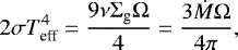 (A.2)
(A.2)
where σ is the Boltzmann constant and  is the Kepler frequency. The corresponding mid-plane temperature is written as
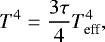 (A.3)
(A.3)
where the optical depth of the gas is written as
 (A.4)
(A.4)
and κ0 is the gas opacity, which we assume to be constant for gas temperatures below the dust sublimation temperature (~ 1300 K). We follow Chambers (2009) in setting κ0 = 3 cm2 g−1.
We scale the mass accretion rate from Eq. (A.1) by the absolute magnitude of the mass accretion rate at the disk edge as follows:
 (A.5)
(A.5)
and combine Eqs. (A.1)–(A.3) such that the mid-plane temperature in the viscously accreting region of the disk is written as
 (A.6)
(A.6)
where
 (A.7)
(A.7)
Further from the host star (r > 10 AU) the gas density is too low for viscous accretion to efficiently heat the disk. Far from the host star the disk is additionally more flared and more easily intersects incoming stellar radiation. The absorption and re-radiation of stellar light is the primary source of heating.
As in Chambers (2009) we follow the model of Chiang & Goldreich (1997) in the irradiated region of the disk (and assume Tgas = Tdust) so that the effective temperature of the gas is written as
![Mathematical equation: \begin{align*} T_{\textrm{eff}} = \left[\frac{r}{2}\frac{\textrm{d}}{\textrm{d}r}\left(\frac{H_{\textrm{ph}}}{r}\right)\right]^{1/4}\left(\frac{R_*}{r}\right)^{1/2} T_*,\end{align*}](/articles/aa/full_html/2019/12/aa36105-19/aa36105-19-eq14.png) (A.8)
(A.8)
where Hph is the height of the photosphere, and R* and T* are the radius and effective temperature of the host star. We assume that the stellar properties remain constant throughout the Class II phase of the proto-stellar system. Assuming that the disk is roughly vertically isothermal then Chiang & Goldreich (1997) found that
 (A.9)
(A.9)
where
 (A.10)
Similarly scaling by the gas properties at the disk outer edge and combining Eqs. (A.8)–(A.10), we find that the mid-plane temperature is written as
 (A.11)
where s0 is the radius of the outer edge of the disk, and
 (A.12)
Both regions of the disk occur concurrently, within a certain radius (rt, known as the heat transition) the heating is dominated by viscous accretion while outwards of the heat transition the heating is dominated by direct irradiation. Such that the disk mid-plane temperature is written as
![Mathematical equation: \begin{align*} T(r) = \begin{cases} T_{\textrm{vis}}\left(\frac{\nu}{\nu_0}\right)^{1/4}\left(\frac{\Sigma_{\textrm{g}}}{\Sigma_0}\right)^{1/2}\left(\frac{\Omega}{\Omega_0}\right)^{1/2} & r < r_{\textrm{t}}, \\[4pt] T_{\textrm{rad}}\left(\frac{r}{s_0}\right)^{-3/7} & r > r_{\textrm{t}}. \end{cases}\end{align*}](/articles/aa/full_html/2019/12/aa36105-19/aa36105-19-eq19.png) (A.13)
(A.13)
To derive the gas surface density we combine the scaled version of Eqs. (A.1) and (A.13) as follows:
![Mathematical equation: \begin{align*} \Sigma_{\textrm{g}}(r) = \begin{cases} \Sigma_{\textrm{vis}}\left(\frac{\dot{M}}{\dot{M}_0}\right)^{3/5}\left(\frac{r}{s_0}\right)^{-3/5} & r < r_{\textrm{t}}, \\[4pt] \Sigma_{\textrm{rad}}\left(\frac{\dot{M}}{\dot{M}_0}\right)\left(\frac{r}{s_0}\right)^{-15/14} & r > r_{\textrm{t}}, \end{cases}\end{align*}](/articles/aa/full_html/2019/12/aa36105-19/aa36105-19-eq20.png) (A.14)
(A.14)
where  and Σrad = Σ0(T0∕Trad). The particular value of Σ0 and T0 depend on the dominate heating source. If viscous accretion dominates at the outer edge of the disk (i.e. Tvis > Trad) then T0 = Tvis, otherwise T0 = Trad. The disk in the former case is characterized by a single power law and the hypothetical location of the heat transition is beyond the edge of the disk (i.e. rt > s0).
In the case in which rt > s0 the normalization Σvis = Σ0 is determined through the initial disk mass as follows:
 (A.15)
while in the case in which rt < s0,
![Mathematical equation: \begin{align*} M_{\textrm{disk},0}= & \int_0^{r_{\textrm{t}}} 2\pi \Sigma_{\textrm{g}}(r < r_{\textrm{t}},t=0) \textrm{d}r \nonumber\\[3pt] &+ \int_{r_{\textrm{t}}}^{s_0} 2\pi\Sigma_{\textrm{g}}(r > r_{\textrm{t}},t=0) \textrm{d}r.\end{align*}](/articles/aa/full_html/2019/12/aa36105-19/aa36105-19-eq23.png) (A.16)
(A.16)
For details see Chambers (2009), we find
![Mathematical equation: \begin{align*} & \Sigma_0 = \Sigma_{\textrm{vis}} = \frac{7M_{\textrm{disk},0}}{10\pi s_0^2} \nonumber\\[3pt] & \Sigma_{\textrm{rad}} = \Sigma_0\frac{T_0}{T_{\textrm{rad}}} \nonumber \end{align*}](/articles/aa/full_html/2019/12/aa36105-19/aa36105-19-eq24.png)
when rt > s0 and
![Mathematical equation: \begin{align*} & \Sigma_0 = \Sigma_{\textrm{rad}} = \frac{13M_{\textrm{disk,0}}}{28\pi s_0^2}\left[1- \frac{33}{98}\left(\frac{T_{\textrm{vis}}}{T_{\textrm{rad}}}\right)^{52/33}\right]^{-1} \nonumber\\[3pt] & \Sigma_{\textrm{vis}} = \Sigma_0\left(\frac{T_0}{T_{\textrm{vis}}}\right)^{4/5} \nonumber \end{align*}](/articles/aa/full_html/2019/12/aa36105-19/aa36105-19-eq25.png)
when rt < s0.
As the disk evolves and the majority of the mass accretes towards the host star, this requires the transport of angular momentum away from the inner disk. When viscous accretion dominates the angular momentum transport, the disk outer edge of the disk (s) spreads outwards from its initial size (s0). Meanwhile if disk winds dominate the evolution, the angular momentum is lifted above the disk as matter flows along magnetic field lines. In this case the outer edge of the disk would not evolve or would tend to shrink. In our work we assume that the outer disk is dominated by viscous angular momentum transport, and hence the outer edge should grow. The angular momentum of the disk is written as
 (A.17)
Combining Eqs. (A.15)–(A.17) we can derive the temporal evolution of the mass accretion rate of the disk. These equations have the form (see Chambers 2009 for details)
![Mathematical equation: \begin{align*} \dot{M}(t) = \begin{cases} \frac{\dot{M}_0}{\left(1 + t/\tau_{\textrm{vis}}\right)^{19/16}} & t < t_1,\\[7pt] \frac{\dot{M}_1}{\left(1 + (t-t_1)/\tau_{\textrm{rad}}\right)^{20/13}} & t > t_1, \end{cases}\end{align*}](/articles/aa/full_html/2019/12/aa36105-19/aa36105-19-eq27.png) (A.18)
(A.18)
where t1 is the time first time when Trad > Tvis, and Ṁ1 is the mass accretion rate at t1. Furthermore τvis = 3M0∕16Ṁ0 and τrad = 7M1∕13Ṁ1 are evolution timescales and M1 is the mass of the disk at t1. In the case in which the outer disk is heated by direct irradiation (i.e. when Trad > Tvis) at the start of the simulation, then t1 = 0.
Along with its viscous accretion, a gas disk is also susceptible to photo-evaporation by far- and extreme-UV photons. The process of photo-evaporation is complicated and a full treatment (i.e. in Gorti et al. 2009, 2015) is beyond the scope of this work. However we account for photo-evaporation using the simpler method outlined in Hasegawa & Pudritz (2013). In their model, photo-evaporation reduces the global mass accretion rate by lifting the gas out of the disk at an exponential rate as follows:
 (A.19)
for t > tint, where tint = 105 yr is the time when the photo-evaporation begins to take effect, and tdep is the depletion timescale from photo-evaporation. As in Alessi & Pudritz (2018) we set the depletion timescale to be equal to the disk lifetime. In this way disks with higher lifetimes have intrinsically lower photo-evaporation rates (by construction) than disks with lower lifetimes.
A.2 Dust model
The distribution and evolution of the dust disk impacts the production and growth of planetesimals via the streaming instability (Schäfer et al. 2017). Additionally, since the volatile freeze-out rate is slower (by mass of dust) for larger grains and larger grains have lower optical depth (per mass of dust) than smaller grains, the average dust grain size also impacts the chemistry in the disk (Jonkheid et al. 2006, 2007; Vasyunin et al. 2011; Fogel et al. 2011; Cridland et al. 2016; Krijt et al. 2016, 2018).
The treatment of the dust evolution in our model is computed with the two-population model of Birnstiel et al. (2012). This model is a semi-analytic approximation that constructs the grain size distribution and dust surface density to replicate the results of numericalsimulations of grain growth and fragmentation. A particularly useful feature of this approach is that it is computationally cheaper to run than full dust simulations, allowing it to be quickly run in support of astrochemical codes and planet formation calculations.
The evolution of the dust is primarily dictated by its Stokes number (St = aρsπ∕2Σg), which describes how much aerodynamic drag a grain of a certain size (a) and density (ρs) feels. For a given grain chemical abundance (and hence density) the Stokes number is limited by three processes: its growth timescale, fragmentation, and radial drift. In the fragmentation limited regime, grains grow to a point at which any subsequent collision leads to erosion rather than grow. The analytic calculations of Birnstiel et al. (2011) have shown that the maximum grain size inthis regime is
 (A.20)
where cs is the gas sound speed. The parameter ff is a factor of order unity, meant to take into account the fact that the actual maximum grain size from numerical simulations is slightly below the maximum size predicted theoretically. A key parameter to this process is the fragmentation threshold speed uf. When two grains impact with speeds above uf they tend to fragment rather than stick together.
Following our past work (Cridland et al. 2017b), we assume that a dust grain with an ice mantle has a fragmentation threshold speed of 10 m s−1. For a dust grain without an ice mantle we assume a fragmentation threshold speed of 1 m s−1. This implies a radial dependence on the fragmentation threshold speed that changes across the water ice line, where water changes its state between vapour and ice.
A second method of limiting the size of the dust grain is through the tension between dust growth and radial drift. When the growth timescale of a grain,
 (A.21)
exceeds the timescale of radial drift (Birnstiel et al. 2012),
 (A.22)
then it drifts inwards faster than it grows. This has an expected maximum grain size of (Birnstiel et al. 2012)
 (A.23)
where Σd is the surface density of the dust and γ is the absolute value of the gas pressure gradient. The parameter fd = 0.55 is set to properly fit the results of the semi-analytic model to numerical simulations.
Because of the transition in fragmentation threshold speed at the water ice line, the combination of fragmentation and radial drift leads to a build up of dust just inside the water ice line. This build up is caused by a reduction in the average grain size inwards of the water ice line. These smaller grains radially drift slower than the grains outwards of the ice line, thereby causing a traffic jam (Pinilla et al. 2016). The increase in dust surface density within the ice line works to increase the efficiency of planetesimal formation and further growth of planets (Dra̧żkowska et al. 2016).
Another important transition point is at the outer edge of the dead zone. The gas turbulence is generally believed to be generated by the magnetorotational instability (MRI; see for ex. Bai & Stone 2013), which requires a high enough electron fraction (ne ∕nH ~ 10−10) for the magnetic field to couple to the bulk gas. At high enough densities, both cosmic rays and high energy photons cannot penetrate enough to supply this level of ionization (Bai & Stone 2011; Gressel et al. 2015). Hence the MRI saturates and the turbulence level drops by about two orders of magnitude (Cridland et al. 2017b).
As was done in Cridland et al. (2017b) we included the effect of an evolving dead zone by dropping αturb to 10−5 within the dead zone. There, the maximum grain size typically becomes dominated by radial drift, since turbulent driven fragmentation becomes much less efficient. We define the location of the dead zone edge through a parametrized model, which was developed in Cridland et al. (2017b). The edge location depends on the ionization structure of the disk gas, as computed by our astrochemical model. Our model assumes a maximum of singly charged dust grains that could underestimate the amount of charge held by the grains, depending on the average size of the dust grains.
A.3 Ultraviolet and X-ray photon field
Along with its impact on planet formation, the dust distribution strongly impacts the flux of high energy radiation. These high energy photons ionize the gas and drive fast chemical reactions in the gas phase. As was done in Cridland et al. (2017b) we combine our dust model described in Sect. A.2 with the radiative transfer scheme RADMC3D Dullemond (2012), following its internal dust opacity calculator to determine the impact of the changing dust distribution on the radiation field. The optical constants used in the opacity calculations were taken from Draine (2003).
For use in our chemical calculation (described below) we pre-compute both the dust radial and size distribution of the dust grains along with the resulting radiation field for a number of different times through the disk. Each of these snapshots are separated in time by on average 105 yr.
Our general method to compute the physical properties of the gas (temperature, density), dust (size, density), and radiation field is to first generate a snapshot of the gas properties at every time step from a starting time of t0 = 105 yr to the end time tfinal = tlife. Next we use the two-population model described above to compute the size and radial distribution of the dust, and assume that it has the same temperature as the gas. Finally we use the gas and dust distributions as inputs to RAMDC3D to compute the high energy radiation field.
With these spatial distributions in hand we compute the chemical structure of the disk for each snapshot (see Sect. 3).
Appendix B: Planet formation
B.1 Planetary growth: planetesimal accretion
The population used in this work is a subset of a population of synthetic planets from Alessi et al. (APC, in prep.). Our subset includes their Zone 1 planets (also known as hot Jupiters/Neptunes), defined by final orbital radii r < 0.1 AU and planetary mass Mp ≥ 10 M⊕ ; and close-in Zone 5 planets (classically called super-Earths or sub-Neptunes) with r < 0.1 AU and Mp < 10 M⊕.
The background model used in APC is featured in Alessi & Pudritz (2018) and was built using the planetesimal accretion paradigm which posits that planets grow through the sequential collisions of large (10–100 km) bodies followed by the accretion of gas after the protoplanet has reached a mass of ~ 10 M⊕. These planetesimals would hypothetically be constructed through the efficient coagulation of pebble-sized grains driven by the streaming instability (see for ex. Schäfer et al. 2017). We do not, however, account for any reduction in the surface density of dust due to the build up of planetesimals. Such an addition would be useful to be consistent with observations of dust mass in protoplanetary disks (Tychoniec et al. 2018), however, we leave it to future work.
This scenario is based on the prescription developed by Kokubo & Ida (2002) and Ida & Lin (2004), and begins with a seed mass of 0.01 M⊕ that accretes planetesimals on a timescale of (Ida & Lin 2004)
![Mathematical equation: \begin{align*} &t_{\textrm{acc}} = 1.2\,{\times}\,10^5\, \textrm{yr} \left(\frac{\Sigma_{\textrm{d}}}{10 \textrm{g~cm}^{-2}}\right)^{-1}\left(\frac{r}{1~\textrm{AU}}\right)^{1/2}\left(\frac{M_{\textrm{c}}}{M_{\oplus}}\right)^{1/3}\nonumber\\ &\quad{\times}\,\left(\frac{M_*}{M_{\odot}}\right)^{-1/6}\left[\left(\frac{\Sigma_{\textrm{g}}}{2.4\,{\times}\,10^3 \,\textrm{g~cm}^{-2}}\right)^{-1/5} \left(\frac{r}{1~\textrm{AU}}\right)^{1/20}\left(\frac{m}{10^{18}\textrm{g}}\right)^{1/15}\right]^2\!,\end{align*}](/articles/aa/full_html/2019/12/aa36105-19/aa36105-19-eq33.png) (B.1)
(B.1)
where Mc and M* are the mass of the protoplanet and host star respectively, while m is the assumed (constant) mass of each of the incoming planetesimals. With this timescale, the protoplanetary mass grows as Ṁc = Mc∕tacc.
At a certain point the protoplanet has accreted or scattered all of its surrounding planetesimals. With the reduction of its associated accretion heating the core becomes sufficiently cool to begin capturing gas. We denote this isolation mass (Alessi & Pudritz 2018)
 (B.2)
(B.2)
where the parameter fcrit depends on the opacity of gas surrounding the protoplanet (Ikoma et al. 2000)
 (B.3)
(B.3)
Alessi & Pudritz (2018) explore different values of κenv and its effect on the resulting population. However for this work we chose κenv = 0.001 cm2g−1 as it represented the population of planets that best reproduced the population of known exoplanets.
As gas accretes it must shed its gravitational energy to remain bound to the planet. The incoming gas cools on the Kelvin–Helmholtz timescale (Ikoma et al. 2000):
 (B.4)
(B.4)
where Mp is the mass of the growing planet and the parameters c and d depend on κenv. Using the expressions from Alessi & Pudritz (2018; their Eqs. (23) and (24)) and κenv = 0.001 cm2g−1: c = 7.7 and d = 2. Assuming that the Kelvin–Helmholtz timescale is the limiting factor to gas accretion then the gas accretion rate is
 (B.5)
(B.5)
While the planet initially accretes gas slowly, as its mass builds it eventually begins a stage of unstable gas accretion. As a final varied parameter in the population synthesis model we set a maximum mass above which a planet stops its growth. As in Alessi & Pudritz (2018) the maximum mass is written as
 (B.6)
(B.6)
where the parameter fmax is stochastically varied between 1 and 500 and Mgap is the gap opening mass. As defined in Matsumura & Pudritz (2006) and Alessi & Pudritz (2018),
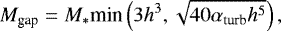 (B.7)
(B.7)
where h = H∕r and H = cs∕Ω is the gas scale height. The first term in Eq. B.7 denotes the point when the hill radius of the planet exceeds the scale height of the disk. At this point the gravitational effect of the planet exceeds the dynamics of the gas. The second term denotes the mass of the planet when its gravitational torque exceeds the viscous torque of the surrounding gas. We assume that when either of these requirements are met that a gap in the disk is opened.
The premise of setting a randomly selected upper limit to the total mass of the planet is a required simplification because of our lack of knowledge of the mechanism responsible for terminating growth. This terminal mass problem was discussed by Morbidelli et al. (2014) who connected the end of planetary growth to gap opening, however found that gas flow into the gap could still be maintained through meridional circulation from heights above the mid-plane. Recently Batygin (2018) hypothesize that this circulating flow could be prevented from accreting onto the planet through complex interactions with the dynamo-driven magnetic field of a planet. With that in mind, Cridland (2018) derive a semi-analytic function for the gas accretion rate, and indeed find that accretion could be stopped with this magnetic shielding. Cridland (2018) derive limits of fmax and found a range between ~100 and 400 for a limited sample of forming planets. Hence our choice in the range of fmax used in this population is reasonable when compared to this physically motivated model. Since the population used in this work is pre-computed by APC we stick to the termination prescribed in Eq. (B.6) and leave the effect on the population of magnetic termination to future work.
B.2 Planetary migration: planet traps
Before it opens a gap, an embedded planet perturbs the surrounding gas as it grows. Numerical simulations (see for ex. Masset 2002) have shown that these perturbations lead to spiral waves in the disk gas that back-react on the planet, predominantly removing its angular momentum. Known as the Lindblad torque, these spiral waves cause the planet to migrate inwards, towards the host star. The Lindblad torque is balanced by the co-rotation torque, that is caused by material orbiting on horseshoe orbits around the planet (Masset et al. 2006; Paardekooper et al. 2010; Lyra et al. 2010; Cridland et al. 2016).
For a simple disk model like the minimum mass solar nebular (MMSN; Crida 2009) the combined effect of the Lindblad and co-rotation torque is inward migration. However more complicated disk models can include transitions in disk properties that strengthen the co-rotation torque producing locations of net zero torque; these are known as “planet traps”. Outlined in Hasegawa & Pudritz (2011), three such planet traps exist in typical protoplanetary disks. They are the water ice line, heat transition, and the edge of the dead zone. These traps represent transitions in the dust opacity by the freeze-out of water, a change in the heating mechanism (discussed above), and a change in the turbulent strength respectively. More recently, Cridland et al. (2019b) use models of astrochemistry, dust opacity, and radiative transfer to rigorously show that these traps indeed lead to a zero point in the net torque on a planet. As in Alessi & Pudritz (2018) we assume thata growing planet is completely trapped in one of these planet traps until they open a gap in the disk.
Once the planet mass exceeds the gap opening mass (Eq. (B.7)) it opens a gap in the gas disk. The planet now begins migrating via Type II migration since the torques responsible for its original Type I migration are switched off by the presence of the gap. Type II migration proceeds at the viscous timescale (tν = r2∕ν), with the planet acting as an intermediary to the global angular momentum transport of the disk. This process continues until the mass interior to the planet falls below the current planetary mass, at which point Type II migration stalls (see Alessi et al. 2017 for details).
References
- Alessi, M., & Pudritz, R. E. 2018, MNRAS, 478, 2599 [NASA ADS] [CrossRef] [Google Scholar]
- Alessi, M., Pudritz, R. E., & Cridland, A. J. 2017, MNRAS, 464, 428 [NASA ADS] [CrossRef] [Google Scholar]
- Ali-Dib, M. 2017, MNRAS, 464, 4282 [NASA ADS] [CrossRef] [Google Scholar]
- Alibert, Y., Mordasini, C., Benz, W., & Winisdoerffer, C. 2005, A&A, 434, 343 [NASA ADS] [CrossRef] [EDP Sciences] [Google Scholar]
- Anderson, D. E., Bergin, E. A., Blake, G. A., et al. 2017, ApJ, 845, 13 [NASA ADS] [CrossRef] [Google Scholar]
- Ansdell, M., Williams, J. P., van der Marel, N., et al. 2016, ApJ, 828, 46 [Google Scholar]
- Atreya, S. K., Crida, A., Guillot, T., et al. 2016, ArXiv e-prints [arXiv:1606.04510] [Google Scholar]
- Bai, X.-N. 2016, ApJ, 821, 80 [Google Scholar]
- Bai, X.-N. 2017, Astrophys. Space Sci. Lib., 445, 63 [NASA ADS] [CrossRef] [Google Scholar]
- Bai, X.-N., & Stone, J. M. 2011, ApJ, 736, 144 [NASA ADS] [CrossRef] [Google Scholar]
- Bai, X.-N., & Stone, J. M. 2013, ApJ, 769, 76 [NASA ADS] [CrossRef] [Google Scholar]
- Baruteau, C., Crida, A., Paardekooper, S.-J., et al. 2014, Protostars and Planets VI (Tucson: University of Arizona Press), 667 [Google Scholar]
- Batygin, K. 2018, AJ, 155, 178 [NASA ADS] [CrossRef] [Google Scholar]
- Benneke, B. 2015, ArXiv e-prints [arXiv:1504.07655] [Google Scholar]
- Benz, W., Ida, S., Alibert, Y., Lin, D., & Mordasini, C. 2014, in Protostars and Planets VI, eds. H. Beuther, R. S. Klessen, C. P. Dullemond, & T. Henning (Tucson: University of Arizona Press), 691 [Google Scholar]
- Bergin, E. A., & Williams, J. P. 2017, in proceedings from conference on Formation, Evolution, and Dynamics of Young Solar Systems, ASSL, 445, 1 [NASA ADS] [CrossRef] [Google Scholar]
- Bergin, E. A., Blake, G. A., Ciesla, F., Hirschmann, M. M., & Li, J. 2015, Proc. Natl. Acad. Sci., 112, 8965 [NASA ADS] [CrossRef] [Google Scholar]
- Bethell, T. J.,& Bergin, E. A. 2011, ApJ, 739, 78 [NASA ADS] [CrossRef] [Google Scholar]
- Birkby, J. L., de Kok, R. J., Brogi, M., Schwarz, H., & Snellen, I. A. G. 2017, AJ, 153, 138 [NASA ADS] [CrossRef] [Google Scholar]
- Birnstiel, T., Klahr, H., & Ercolano, B. 2012, A&A, 539, A148 [NASA ADS] [CrossRef] [EDP Sciences] [Google Scholar]
- Birnstiel, T., Windmark, F., Dullemond, C. P., & Klahr, H. 2011, Lunar Planet. Institute Contrib., 1639, 9063 [NASA ADS] [Google Scholar]
- Bitsch, B., Lambrechts, M., & Johansen, A. 2015, A&A, 582, A112 [NASA ADS] [CrossRef] [EDP Sciences] [Google Scholar]
- Booth, R. A., & Ilee, J. D. 2019, MNRAS, 487, 3998 [NASA ADS] [CrossRef] [Google Scholar]
- Booth, R. A., Clarke, C. J., Madhusudhan, N., & Ilee, J. D. 2017, MNRAS, 469, 3994 [NASA ADS] [CrossRef] [Google Scholar]
- Booth, A. S., Walsh, C., Ilee, J. D., et al. 2019, ApJ, 882, L31 [NASA ADS] [CrossRef] [Google Scholar]
- Bosman, A. D., Tielens, A. G. G. M., & van Dishoeck, E. F. 2018a, A&A, 611, A80 [NASA ADS] [CrossRef] [EDP Sciences] [Google Scholar]
- Bosman, A. D., Walsh, C., & van Dishoeck, E. F. 2018b, A&A, 618, A182 [NASA ADS] [CrossRef] [EDP Sciences] [Google Scholar]
- Brewer, J. M., & Fischer, D. A. 2016, ApJ, 831, 20 [NASA ADS] [CrossRef] [Google Scholar]
- Brewer, J. M., Fischer, D. A., & Madhusudhan, N. 2017, AJ, 153, 83 [NASA ADS] [CrossRef] [Google Scholar]
- Brogi, M., Snellen, I. A. G., de Kok, R. J., et al. 2013, ApJ, 767, 27 [NASA ADS] [CrossRef] [Google Scholar]
- Brogi, M., de Kok, R. J., Birkby, J. L., Schwarz, H., & Snellen, I. A. G. 2014, A&A, 565, A124 [NASA ADS] [CrossRef] [EDP Sciences] [Google Scholar]
- Brogi, M., de Kok, R. J., Albrecht, S., et al. 2016, ApJ, 817, 106 [NASA ADS] [CrossRef] [Google Scholar]
- Chambers, J. E. 2009, ApJ, 705, 1206 [NASA ADS] [CrossRef] [Google Scholar]
- Chambers, J. 2018, ApJ, 865, 30 [NASA ADS] [CrossRef] [Google Scholar]
- Chiang, E. I., & Goldreich, P. 1997, ApJ, 490, 368 [NASA ADS] [CrossRef] [Google Scholar]
- Ciesla, F. J., & Cuzzi, J. N. 2006, Icarus, 181, 178 [NASA ADS] [CrossRef] [Google Scholar]
- Cleeves, L. I., Bergin, E. A., & Adams, F. C. 2014, ApJ, 794, 123 [NASA ADS] [CrossRef] [Google Scholar]
- Cleeves, L. I., Öberg, K. I., Wilner, D. J., et al. 2018, ApJ, 865, 155 [NASA ADS] [CrossRef] [Google Scholar]
- Crida, A. 2009, ApJ, 698, 606 [NASA ADS] [CrossRef] [Google Scholar]
- Cridland, A. J. 2018, A&A, 619, A165 [NASA ADS] [CrossRef] [EDP Sciences] [Google Scholar]
- Cridland, A. J., Pudritz, R. E., & Alessi, M. 2016, MNRAS, 461, 3274 [Google Scholar]
- Cridland, A. J., Pudritz, R. E., Birnstiel, T., Cleeves, L. I., & Bergin, E. A. 2017a, MNRAS, 469, 3910 [NASA ADS] [CrossRef] [Google Scholar]
- Cridland, A. J., Pudritz, R. E., & Birnstiel, T. 2017b, MNRAS, 465, 3865 [NASA ADS] [CrossRef] [Google Scholar]
- Cridland, A. J., Eistrup, C., & van Dishoeck, E. F. 2019a, A&A, 627, A127 [NASA ADS] [CrossRef] [EDP Sciences] [Google Scholar]
- Cridland, A. J., Pudritz, R. E., & Alessi, M. 2019b, MNRAS, 484, 345 [NASA ADS] [CrossRef] [Google Scholar]
- Davies, M. B., Adams, F. C., Armitage, P., et al. 2014, in Protostars and Planets VI, eds. H. Beuther, R. S. Klessen, C. P. Dullemond, & T. Henning (Tucson: University of Arizona Press), 787 [Google Scholar]
- Draine, B. T. 2003, ApJ, 598, 1026 [NASA ADS] [CrossRef] [Google Scholar]
- Dra̧żkowska, J., & Alibert, Y. 2017, A&A, 608, A92 [NASA ADS] [CrossRef] [EDP Sciences] [Google Scholar]
- Dra̧żkowska, J., Alibert, Y., & Moore, B. 2016, A&A, 594, A105 [NASA ADS] [CrossRef] [EDP Sciences] [Google Scholar]
- Drozdovskaya, M. N., Walsh, C., Visser, R., Harsono, D., & van Dishoeck, E. F. 2014, MNRAS, 445, 913 [NASA ADS] [CrossRef] [Google Scholar]
- Dullemond, C. P. 2012, Astrophysics Source Code Library [record ascl:1202.015] [Google Scholar]
- Eistrup, C., Walsh, C., & van Dishoeck, E. F. 2016, A&A, 595, A83 [NASA ADS] [CrossRef] [EDP Sciences] [Google Scholar]
- Eistrup, C., Walsh, C., & van Dishoeck, E. F. 2018, A&A, 613, A14 [NASA ADS] [CrossRef] [EDP Sciences] [Google Scholar]
- Espinoza, N., Fortney, J. J., Miguel, Y., Thorngren, D., & Murray-Clay, R. 2017, ApJ, 838, L9 [Google Scholar]
- Favre, C., Cleeves, L. I., Bergin, E. A., Qi, C., & Blake, G. A. 2013, ApJ, 776, L38 [NASA ADS] [CrossRef] [Google Scholar]
- Feng, Y. K., Line, M. R., Fortney, J. J., et al. 2016, ApJ, 829, 52 [NASA ADS] [CrossRef] [Google Scholar]
- Fogel, J. K. J., Bethell, T. J., Bergin, E. A., Calvet, N., & Semenov, D. 2011, ApJ, 726, 29 [NASA ADS] [CrossRef] [Google Scholar]
- Gail, H.-P., & Trieloff, M. 2017, A&A, 606, A16 [NASA ADS] [CrossRef] [EDP Sciences] [Google Scholar]
- Gandhi, S., & Madhusudhan, N. 2018, MNRAS, 474, 271 [Google Scholar]
- Goldreich, P., & Tremaine, S. 1979, ApJ, 233, 857 [NASA ADS] [CrossRef] [MathSciNet] [Google Scholar]
- Gomes, R., Levison, H. F., Tsiganis, K., & Morbidelli, A. 2005, Nature, 435, 466 [NASA ADS] [CrossRef] [PubMed] [Google Scholar]
- Gorti, U., Dullemond, C. P., & Hollenbach, D. 2009, ApJ, 705, 1237 [NASA ADS] [CrossRef] [Google Scholar]
- Gorti, U., Hollenbach, D., & Dullemond, C. P. 2015, ApJ, 804, 29 [NASA ADS] [CrossRef] [Google Scholar]
- Gressel, O., Turner, N. J., Nelson, R. P., & McNally, C. P. 2015, ApJ, 801, 84 [NASA ADS] [CrossRef] [Google Scholar]
- Hasegawa, Y., & Pudritz, R. E. 2011, MNRAS, 417, 1236 [NASA ADS] [CrossRef] [Google Scholar]
- Hasegawa, Y., & Pudritz, R. E. 2013, ApJ, 778, 78 [NASA ADS] [CrossRef] [Google Scholar]
- Helling, C., Woitke, P., Rimmer, P. B., et al. 2014, Life, 4, 142 [NASA ADS] [CrossRef] [Google Scholar]
- Heng, K., & Marley, M. S. 2018, Handbook of Exoplanet, Radiative Transfer for Exoplanet Atmospheres (Berlin: Springer), 102 [Google Scholar]
- Ida, S., & Lin,D. N. C. 2004, ApJ, 604, 388 [NASA ADS] [CrossRef] [PubMed] [Google Scholar]
- Ikoma, M., Nakazawa, K., & Emori, H. 2000, ApJ, 537, 1013 [NASA ADS] [CrossRef] [Google Scholar]
- Johansen, A., Oishi, J. S., Mac Low, M.-M., et al. 2007, Nature, 448, 1022 [Google Scholar]
- Jonkheid, B., Dullemond, C. P., Hogerheijde, M. R., & van Dishoeck, E. F. 2007, A&A, 463, 203 [NASA ADS] [CrossRef] [EDP Sciences] [Google Scholar]
- Jonkheid, B., Kamp, I., Augereau, J. C., & van Dishoeck, E. F. 2006, A&A, 453, 163 [NASA ADS] [CrossRef] [EDP Sciences] [Google Scholar]
- Kama, M., Bruderer, S., Carney, M., et al. 2016, A&A, 588, A108 [NASA ADS] [CrossRef] [EDP Sciences] [Google Scholar]
- Klarmann, L., Ormel, C. W., & Dominik, C. 2018, A&A, 618, L1 [NASA ADS] [CrossRef] [EDP Sciences] [Google Scholar]
- Kokubo, E., & Ida, S. 2002, ApJ, 581, 666 [NASA ADS] [CrossRef] [Google Scholar]
- Kreidberg, L., Bean, J. L., Désert, J.-M., et al. 2014, ApJ, 793, L27 [NASA ADS] [CrossRef] [Google Scholar]
- Krijt, S., Ciesla, F. J., & Bergin, E. A. 2016, ApJ, 833, 285 [NASA ADS] [CrossRef] [Google Scholar]
- Krijt, S., Schwarz, K. R., Bergin, E. A., & Ciesla, F. J. 2018, ApJ, 864, 78 [NASA ADS] [CrossRef] [Google Scholar]
- Lin, D. N. C., & Papaloizou, J. 1986, ApJ, 309, 846 [NASA ADS] [CrossRef] [Google Scholar]
- Line, M. R., Knutson, H., Wolf, A. S., & Yung, Y. L. 2014, ApJ, 783, 70 [NASA ADS] [CrossRef] [Google Scholar]
- Lyra, W., Paardekooper, S.-J., & Mac Low, M.-M. 2010, ApJ, 715, L68 [NASA ADS] [CrossRef] [Google Scholar]
- MacDonald, R. J., & Madhusudhan, N. 2019, MNRAS, 486, 1292 [NASA ADS] [CrossRef] [Google Scholar]
- Madhusudhan, N. 2012, ApJ, 758, 36 [NASA ADS] [CrossRef] [Google Scholar]
- Madhusudhan, N., & Seager, S. 2011, ApJ, 729, 41 [NASA ADS] [CrossRef] [Google Scholar]
- Madhusudhan, N., Amin, M. A., & Kennedy, G. M. 2014, ApJ, 794, L12 [Google Scholar]
- Madhusudhan, N., Amin, M. A., & Kennedy, G. M. 2019, MNRAS, 486, 1292 [NASA ADS] [CrossRef] [Google Scholar]
- Madhusudhan, N., Bitsch, B., Johansen, A., & Eriksson, L. 2017, MNRAS, 469, 4102 [NASA ADS] [CrossRef] [Google Scholar]
- Masset, F. S. 2002, A&A, 387, 605 [NASA ADS] [CrossRef] [EDP Sciences] [Google Scholar]
- Masset, F. S., & Papaloizou, J. C. B. 2003, ApJ, 588, 494 [NASA ADS] [CrossRef] [Google Scholar]
- Masset, F. S., Morbidelli, A., Crida, A., & Ferreira, J. 2006, ApJ, 642, 478 [NASA ADS] [CrossRef] [Google Scholar]
- Matsumura, S., & Pudritz, R. E. 2006, MNRAS, 365, 572 [NASA ADS] [CrossRef] [Google Scholar]
- Miller, N., & Fortney, J. J. 2011, ApJ, 736, L29 [NASA ADS] [CrossRef] [Google Scholar]
- Milliner, K., Matthews, J. H., Long, K. S., & Hartmann, L. 2019, MNRAS, 483, 1663 [NASA ADS] [CrossRef] [Google Scholar]
- Miotello, A., van Dishoeck, E. F., Kama, M., & Bruderer, S. 2016, A&A, 594, A85 [NASA ADS] [CrossRef] [EDP Sciences] [Google Scholar]
- Mishra, A., & Li, A. 2015, ApJ, 809, 120 [NASA ADS] [CrossRef] [Google Scholar]
- Moll, R., Garaud, P., Mankovich, C., & Fortney, J. J. 2017, ApJ, 849, 24 [Google Scholar]
- Morbidelli, A. 2018, Handbook of Exoplanets (Berlin: Springer International Publishing AG) 145 [Google Scholar]
- Mordasini, C., Alibert, Y., & Benz, W. 2009a, A&A, 501, 1139 [NASA ADS] [CrossRef] [EDP Sciences] [Google Scholar]
- Mordasini, C., Alibert, Y., Benz, W., & Naef, D. 2009b, A&A, 501, 1161 [NASA ADS] [CrossRef] [EDP Sciences] [Google Scholar]
- Morbidelli, A., Szulágyi, J., Crida, A., et al. 2014, Icarus, 232, 266 [NASA ADS] [CrossRef] [Google Scholar]
- Mordasini, C., Mollière, P., Dittkrist, K.-M., Jin, S., & Alibert, Y. 2015, Int. J. Astrobiol., 14, 201 [CrossRef] [Google Scholar]
- Mordasini, C., van Boekel, R., Mollière, P., Henning, T., & Benneke, B. 2016, ApJ, 832, 41 [NASA ADS] [CrossRef] [Google Scholar]
- Morley, C. V., Knutson, H., Line, M., et al. 2017, AJ, 153, 86 [NASA ADS] [CrossRef] [Google Scholar]
- Moses, J. I., Madhusudhan, N., Visscher, C., & Freedman, R. S. 2013, ApJ, 763, 25 [NASA ADS] [CrossRef] [Google Scholar]
- Mousis, O., Madhusudhan, N., Johnson, T. V., & Lunine, J. I. 2011, in EPSC-DPS Joint Meeting 2011, 2011, 371 [NASA ADS] [Google Scholar]
- Najita, J. R., & Bergin, E. A. 2018, ApJ, 864, 168 [Google Scholar]
- Öberg, K. I., Murray-Clay, R., & Bergin, E. A. 2011, ApJ, 743, L16 [NASA ADS] [CrossRef] [Google Scholar]
- Ormel, C. W., & Klahr, H. H. 2010, A&A, 520, A43 [NASA ADS] [CrossRef] [EDP Sciences] [Google Scholar]
- Paardekooper,S.-J., Baruteau, C., Crida, A., & Kley, W. 2010, MNRAS, 401, 1950 [NASA ADS] [CrossRef] [Google Scholar]
- Paardekooper,S.-J., Baruteau, C., & Kley, W. 2011, MNRAS, 410, 293 [NASA ADS] [CrossRef] [Google Scholar]
- Pascucci, I., Andrews, S., Chandler, C., & Isella, A. 2018, ASP Conf. Ser., 517, 155 [NASA ADS] [Google Scholar]
- Pinhas, A., Madhusudhan, N., Gandhi, S., & MacDonald, R. 2019, MNRAS, 482, 1485 [Google Scholar]
- Pinilla, P., Klarmann, L., Birnstiel, T., et al. 2016, A&A, 585, A35 [NASA ADS] [CrossRef] [EDP Sciences] [Google Scholar]
- Pontoppidan, K. M., Salyk, C., Bergin, E. A., et al. 2014, Protostars and Planets VI (Tucson: University of Arizona Press), 363 [Google Scholar]
- Rimmer, P. B., & Helling, C. 2016, ApJS, 224, 9 [NASA ADS] [CrossRef] [Google Scholar]
- Schäfer, U., Yang, C.-C., & Johansen, A. 2017, A&A, 597, A69 [NASA ADS] [CrossRef] [EDP Sciences] [Google Scholar]
- Schwarz, K. R., Bergin, E. A., Cleeves, L. I., et al. 2018, ApJ, 856, 85 [NASA ADS] [CrossRef] [Google Scholar]
- Schwarz, K. R., Bergin, E. A., Cleeves, L. I., et al. 2019, ApJ, 877, 131 [NASA ADS] [CrossRef] [Google Scholar]
- Shakura, N. I., & Sunyaev, R. A. 1973, A&A, 24, 337 [NASA ADS] [Google Scholar]
- Smith, I. W. M., Herbst, E., & Chang, Q. 2004, MNRAS, 350, 323 [NASA ADS] [CrossRef] [Google Scholar]
- Stevenson, K. B., Bean, J. L., Seifahrt, A., et al. 2014, AJ, 147, 161 [NASA ADS] [CrossRef] [Google Scholar]
- Tazzari, M., Testi, L., Natta, A., et al. 2017, A&A, 606, A88 [NASA ADS] [CrossRef] [EDP Sciences] [Google Scholar]
- Thiabaud, A., Marboeuf, U., Alibert, Y., Leya, I., & Mezger, K. 2015, A&A, 574, A138 [NASA ADS] [CrossRef] [EDP Sciences] [Google Scholar]
- Thorngren, D., & Fortney, J. J. 2019, ApJ, 874, L31 [NASA ADS] [CrossRef] [Google Scholar]
- Thorngren, D. P., Fortney, J. J., Murray-Clay, R. A., & Lopez, E. D. 2016, ApJ, 831, 64 [NASA ADS] [CrossRef] [Google Scholar]
- Tychoniec, Ł., Tobin, J. J., Karska, A., et al. 2018, ApJS, 238, 19 [NASA ADS] [CrossRef] [Google Scholar]
- Vasyunin, A. I., Wiebe, D. S., Birnstiel, T., et al. 2011, ApJ, 727, 76 [NASA ADS] [CrossRef] [Google Scholar]
- Wahl, S. M., Hubbard, W. B., Militzer, B., et al. 2017, Geophys. Res. Lett., 44, 4649 [NASA ADS] [CrossRef] [Google Scholar]
- Walsh, C., Millar, T. J., Nomura, H., et al. 2014, A&A, 563, A33 [NASA ADS] [CrossRef] [EDP Sciences] [Google Scholar]
- Wang, L., Bai, X.-N., & Goodman, J. 2019, ApJ, 874, 90 [NASA ADS] [CrossRef] [Google Scholar]
- Ward, W. R. 1991, Lunar Planet. Sci. Conf., 22, 1463 [NASA ADS] [Google Scholar]
- Wei, C.-E., Nomura, H., Lee, J.-E., et al. 2019, ApJ, 870, 129 [NASA ADS] [CrossRef] [Google Scholar]
- Yu, M., Evans, N. J., I., Dodson-Robinson, S. E., Willacy, K., & Turner, N. J. 2017, ApJ, 841, 39 [NASA ADS] [CrossRef] [Google Scholar]
- Zheng, X., Kouwenhoven, M. B. N., & Wang, L. 2015, MNRAS, 453, 2759 [NASA ADS] [CrossRef] [Google Scholar]
All Tables
Parameters for the distributions used to select initial conditions in the APC population.
Observed C/O and/or inferred ranges of possible C/O for planets that orbit at < 0.1 AU.
All Figures
|
Fig. 1 Range of disk initial masses and lifetimes for the planet sub-population from APC used in this work. |
| In the text | |
|
Fig. 2 Comparison of distribution of disk masses in our population of Zone 1 planets, evolved using the model presented in Sect. A.1. We show the mass of each of the disk models at its initial time, 2, 4, and 6 Myr into their evolution, even if the disk lifetime for any particular disk model is shorter than those times. We compare to the disk masses measured in a population of class 0/I from Tychoniec et al. (2018) and to a population of class II objects from Ansdell et al. (2016). |
| In the text | |
|
Fig. 3 Example of how physical properties of disk evolve between 0.5 and 0.7 Myr at a radius of 10 AU. The gas temperature, abundance of water ice, and UV flux are measured at the disk mid-plane. The gas temperature and density, dust density, and flux high energy radiation stay constant during a single time step. These values are then adjusted to a new value at the end of the timestep before the chemical evolution moves onwards in time. |
| In the text | |
|
Fig. 4 Mid-plane distribution of primary carbon and oxygen bearing volatile molecules as computed by the original Michigan chemical code (passive disk) and our modified version (evolving disk). The label “(gr)” denotes molecules that are frozen on the dust grains. Each model is run up to 1 Myr, however in the evolving model the disk temperature and gas surface density evolves with time. |
| In the text | |
|
Fig. 5 Carbon to oxygen ratio (C/O) of gas and dust (ice and refractories) for a disk model in our population. The gas disk has a higher C/O than unity for ~ 0.5 Myr until the disk has cooled slightly. The ice is almost exclusively oxygen rich, apart from a region of the inner disk at late times caused by the slow production and freeze-out of long chain hydrocarbons. We included the excess carbon from the reset model, which eventually disappears after nearly 0.8 Myr. The solids in the region of the disk in which the carbonaceous dust is eroded is always oxygen rich, since the silicates remain in the dust grain while the carbon is removed. C/O changes most at the ice lines of the disk, particularly the water ice line between 2 and 3 AU. The CO ice line is located outside of 60 AU, and hence does not show up in the figure. |
| In the text | |
|
Fig. 6 Test population of hot Jupiters and close-in super-Earths taken from APC. This population covers a wide range of final radii and mass. We note whether the planet grew in the dead zone, water ice line, heat transition (heat trans), and lifetime of the disk in which the planets grew. |
| In the text | |
|
Fig. 7 Carbon-to-oxygen ratio for the population of planets assuming that gas accretion is the sole source of carbon and oxygen in the atmosphere. The vertical dashed line denotes the C/O of the gas disk, which the majority of planets mimic. |
| In the text | |
|
Fig. 8 Carbon-to-oxygen ratio for the case including solid accretion into the atmosphere, but ignore the excess carbon in the gas phase. As such, solid accretion predominately delivers oxygen-rich silicates and ices to the exoplanetary atmospheres. |
| In the text | |
|
Fig. 9 Starting radii of the planets in our population. Generally the planets trapped at the ice line begin within a small range of radii since the location of the ice line is only weakly dependent on initial disk mass. We note that planets that start between 10 and 20 AU do not end their evolution as hot-Jupiter or close-in super-Earths, hence the deficit of points. |
| In the text | |
|
Fig. 10 Same as figure Fig. 8 but for the reset model (panel a) of carbon excess with a constant net advection speed of 6.32 AU Myr−1 as prescribed by hydrodynamic disk models. As such, some planets reach a region of the disk at which the excess carbon remains in the gas phase in time to incorporate it into its atmosphere. For the ongoing model (panel b) the net flux of the excess carbon is zero, which keeps a high carbon abundance. As such most of the planets reach a region of the disk at which the carbon is enhanced owing to the ongoing processing of dust grains. |
| In the text | |
|
Fig. 11 Main sequence of C/O for the planet in our population. Over a wide range of masses we find that lower C/O is caused by the total mass of planet coming predominantly from solid (refractory) sources. The exception comes from the low mass planets (M < 10 M⊕), which are not chemically affected by the accretion of planetesimals. |
| In the text | |
|
Fig. 12 Mass-metallicity relation for two tracers O/H (panel a) and Si/H (panel b). We similarly show the metallicity for the solar system giants (inferred by methane abundance and taken from Kreidberg et al. 2014), WASP-43 b (Kreidberg et al. 2014), GJ 436 b (Morley et al. 2017), and HAT-P-26 b (MacDonald & Madhusudhan 2019) from their water abundance. We find that our Neptune-mass planets are consistent with the metallicity of HAT-P-26 b, but not with Uranus or Neptune, suggesting the formation location could be important to O/H. The Si/H spread in metallicity for a given planet mass is caused by the accretion of solids. In this case our Neptune-mass planets are consistent with the inferred metallicity of Uranus and Neptune. |
| In the text | |
|
Fig. 13 Comparing the observed atmospheric C/O (black) shown in Table 3 to our population of planets. Each line segment represents the shift in C/O between the carbon excess models shown in Figs. 10a and b for each synthetic planet. Additionally we include an increase in C/O in Neptune GJ 436 b-like planets caused by a rain of silicates (dashed line; see the text). |
| In the text | |
Current usage metrics show cumulative count of Article Views (full-text article views including HTML views, PDF and ePub downloads, according to the available data) and Abstracts Views on Vision4Press platform.
Data correspond to usage on the plateform after 2015. The current usage metrics is available 48-96 hours after online publication and is updated daily on week days.
Initial download of the metrics may take a while.