| Issue |
A&A
Volume 631, November 2019
|
|
|---|---|---|
| Article Number | A136 | |
| Number of page(s) | 8 | |
| Section | Planets and planetary systems | |
| DOI | https://doi.org/10.1051/0004-6361/201936464 | |
| Published online | 06 November 2019 | |
Precise radial velocities of giant stars
XIII. A second Jupiter orbiting in 4:3 resonance in the 7 CMa system★,★★,★★★
1
Instituto de Astrofísica de Canarias (IAC),
38205 La Laguna,
Tenerife,
Spain
e-mail: This email address is being protected from spambots. You need JavaScript enabled to view it.
2
Departamento de Astrofísica, Universidad de La Laguna (ULL),
38206
La Laguna,
Tenerife, Spain
3
Landessternwarte, Zentrum für Astronomie der Universität Heidelberg,
Königstuhl 12,
69117 Heidelberg, Germany
4
Max-Planck-Institut für Astronomie,
Königstuhl 17,
69117 Heidelberg, Germany
5
Department of Earth Sciences, The University of Hong Kong,
Pokfulam Road, Hong Kong
6
Department of Physics, The University of Hong Kong,
Pokfulman Road, Hong Kong
7
Stellar Astrophysics Centre, Department of Physics and Astronomy, Aarhus University,
Ny Munkegade 120,
8000 Aarhus C, Denmark
8
Department of Physics and Astronomy, Macquarie University,
North Ryde,
NSW 2109, Australia
Received:
6
August
2019
Accepted:
8
October
2019
Abstract
We report the discovery of a second planet orbiting the K giant star 7 CMa based on 166 high-precision radial velocities obtained with Lick, HARPS, UCLES, and SONG. The periodogram analysis reveals two periodic signals of approximately 745 and 980 d, associated with planetary companions. A double-Keplerian orbital fit of the data reveals two Jupiter-like planets with minimum masses mb sini ~ 1.9 MJ and mc sini ~ 0.9 MJ, orbiting at semimajor axes of ab ~ 1.75 au and ac ~ 2.15 au, respectively. Given the small orbital separation and the large minimum masses of the planets, close encounters may occur within the time baseline of the observations; thus, a more accurate N-body dynamical modeling of the available data is performed. The dynamical best-fit solution leads to collision of the planets and we explore the long-term stable configuration of the system in a Bayesian framework, confirming that 13% of the posterior samples are stable for at least 10 Myr. The result from the stability analysis indicates that the two planets are trapped in a low-eccentricity 4:3 mean motion resonance. This is only the third discovered system to be inside a 4:3 resonance, making this discovery very valuable for planet formation and orbital evolution models.
Key words: techniques: radial velocities / planetary systems / planets and satellites: dynamical evolution and stability / planets and satellites: detection
RV data are only available at the CDS via anonymous ftp to cdsarc.u-strasbg.fr (130.79.128.5) or via http://cdsarc.u-strasbg.fr/viz-bin/cat/J/A+A/631/A136
Based on observations collected at Lick Observatory, University of California.
Based on observations collected at the European Organization for Astronomical Research in the Southern Hemisphere under ESO programmes 078.C-0751, 079.C-0657, 081.C-0802, 082.C-0427, 289.C-5053, 0100.C-0414 and 0101.C-0232.
© ESO 2019
1 Introduction
Today, about 4000 exoplanets around about roughly 3000 host stars are known. Most have been found with the transiting method, while 529 systems so far have been discovered via Doppler monitoring. Surprisingly, the fraction of multi-planetary systems discovered with each method is about the same, i.e., around 23% according to the NASA Exoplanet Archive1. The transit method, however, can only discover those systems which are rather well aligned, while there is no strong bias against planets orbiting in tilted planes with respect to each other with the Doppler method. However, the apparent excess of single transiting systems has led some authors to speculate about the existence of a population of intrinsic singles or highly inclined multi-planetsystems (Lissauer et al. 2011; Ballard & Johnson 2016).
These numbers are lower limits on the number of multi-planetary systems; this is because many planets presumably remain hidden evenin the known systems since they are harder to detect owing to lower masses and/or larger periods. Furthermore, it has been shown that sparse radial velocity (RV) sampling, especially of systems in 2:1 mean motion resonance (MMR), is prone to missing the second planet, and instead makes the system appear as if it only hosts a single eccentric planet (Anglada-Escudé et al. 2010; Kürster et al. 2015; Boisvert et al. 2018; Wittenmyer et al. 2019).
We carried out a Doppler survey for planets around 373 intermediate-mass evolved stars at Lick Observatory from 1999 to 2011 (Frink et al. 2001, 2002) and are currently following up some of the most compelling systems with SONG (Grundahl et al. 2007, 2017). In this work, we report on K1 III giant 7 CMa, one particular system from the Lick survey, which we followed up with the High Accuracy Radial velocity Planet Searcher (HARPS) and the Stellar Observations Network Group (SONG) spectrographs.
One giant planet, namely 7 CMa b, was already reported to orbit 7 CMa by Schwab (2010). It was independently found by Wittenmyer et al. (2011) based on RV data covering about one orbital cycle. Our data, covering about nine orbital cycles, indicate the presence of another giant planet in the system in a 4:3 MMR with the inner companion. Thus, 7 CMa is part of an elusive list of multi-planetary systems with giant host stars, some of which are close to first-order MMRs, as discussed in Trifonov et al. (2019). From the Lick sample, other MMR systems include η Cet (2:1; Trifonov et al. 2014)and ν Oph (6:1; Quirrenbach et al. 2019).
Multi-planetary systems, and especially those in MMR, tell us much more about planet formation than single planet systems. The formation of a 4:3 MMR is especially hard to explain (Rein et al. 2012) with current models since the systems have to move through the 2:1 and 3:2 commensurabilities on their way to the 4:3 resonance, where the two planets are rather close together. 7 CMa is only the third system found in 4:3 MMR via Doppler monitoring, next to HD 200964 (Johnson et al. 2011) and HD 5319 (Giguere et al. 2015), involving massive, Jovian-like planets. All three systems are found around evolved host stars, in the late subgiant or early giant star phases, that are more massive than the Sun and with stellar radii in a narrow range between 4 and 5 R⊙. Thus, the discovery of more systems in the 4:3 MMR will certainly help to shed light on the formation mechanism of those and potentially other systems.
The paper is organized as follows: Sect. 2 is dedicated to the stellar parameters of 7 CMa, while in Sect. 3 we describe our RV dataset. Section 4 provides a dynamical analysis of the system, and in Sect. 5 we discuss the system and possible implications for its formation theory.
2 Host star
7 CMa (= HD 47205, HIP 31592) is a bright K1 giant in the constellation Canis Major that is accessible from most sites in both hemispheres. Comparing spectroscopic, photometric, and astrometric observables to grids of stellar evolutionary models using Bayesian inference, Stock et al. (2018) have derived an effective temperature of 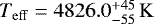 and surface gravity of
 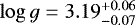 . The metallicity was fixed to the value of [Fe∕H] = 0.21 ± 0.1 from Hekker & Meléndez (2007). The derived mass and radius of 7 CMa are
 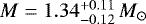 and
and 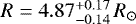 . Table 1 summarizes the main parameters of this star and previous values reported in the literature.
To illustrate the expected evolutionary stage of the host star, we interpolated within the PARSEC grid of evolutionary tracks (Bressan et al. 2012) to obtain a track corresponding to the determined mass and metallicity of the star, which is shown in Fig. 1. The momentary position of 7 CMa according to its temperature and luminosity is on the early ascent of the red giant branch (RGB), hence fusing hydrogen in a shell around an inert helium core. The star undergoes a helium flash, which happens on a timescale that is too short to be covered in the entries of the track. Therefore, the evolution along the black line running from the RGB tip to the beginning of the horizontal branch takes place quasi-instantly.
To date, one confirmed planet is already known to orbit 7 CMa. This planetary system was studied by Schwab (2010) using Lick RVs and is the first reported discovery from the Pan-Pacific Planet Search survey (Wittenmyer et al. 2011) at the 3.9 m Anglo-Australian Telescope using the UCLES (University College London Echelle Spectrograph) spectrograph. Wittenmyer et al. (2011) announced a giant planet (mb sini = 2.6 MJ) with a period of Pb = 763 ± 17 d and eccentricity eb = 0.14 ± 0.06, based on 21RV measurements taken between 2009 and 2011 with UCLES, adopting a stellar mass of 1.52 ± 0.30 M⊙. Later, in a paper published together with another five discoveries, Wittenmyer et al. (2016) presented updated velocities and a refined orbitfor 7 CMa together with six more measurements. The amplitude of the Doppler signal was also confirmed to be independentof wavelength, as expected for a planetary companion, by Trifonov et al. (2015) using near-infrared RVs obtained with CRIRES.
Stellar parameters of 7 CMa.
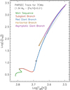 |
Fig. 1 Interpolated evolutionary track for 7 CMa in the Hertzsprung–Russell diagram. The different evolutionary phases are color-coded. The sluminosity and temperature of the star, including uncertainties, are shown in black. |
3 Radial velocity measurements
We collected RVs of 7 CMa from four different instruments during the last 19 yr as part of the project “Precise radial velocities of giant stars”. In the following subsections, a short description of each instrument dataset is presented.
3.1 Lick dataset
Starting in 1999, our group carried out a RV survey of 373 G- and K-giants at Lick Observatory using the 0.6 m Coudé Auxiliary Telescope (CAT) together with the Hamilton Echelle Spectrograph with a nominal resolution of R ~ 60 000 (see, e.g., Frink et al. 2002; Reffert et al. 2006, for a description of the survey and earlier results). Using the iodine cell method as described by Butler et al. (1996) we obtained a typical RV precision of σjitt,Lick = 5–8 ms−1, which is adequate enough for our survey (Reffert et al. 2015). A total of 65 spectra for 7 CMa were taken between September 2000 and November 2011. The resulting RV measurements have a median precision of ~5 ms−1.
3.2 HARPS dataset
We observed 7 CMa with the echelle optical spectrograph HARPS installed at the European Southern Observatory (ESO) 3.6 m telescope at La Silla Observatory in Chile. We retrieved 11 measurements from 2006 to 2009 from the ESO Archive. Then, we triggered a campaign of 12 observations spanning three months in 2013, and five additional nights in March, April, and September 2018. In this last campaign we took a series of consecutive exposures to study the intrinsic stellar variability (jitter) of the star. In total, 127 spectra were obtained.
Radial velocities were obtained with the SERVAL program (Zechmeister et al. 2018) using high signal-to-noise templates created by co-adding all available spectra of the star. We split the HARPS data into two separate temporal subsets, HARPS-pre and HARPS-post, owing to the HARPS fiber upgrade in June 2015, which introduced an RV offset that has to be modeled in the fitting process (Lo Curto et al. 2015). In summary, a total of 25 nightly averaged RVs (20 HARPS-pre and 5 HARPS-post) with a mean internal velocity uncertainty of σHARPS ~ 1 ms−1 were used in the analysis.
3.3 SONG dataset
The SONG collaboration is planned as a network of 1 m telescopes in both hemispheres that carries out high-precision RV measurements of stars. The first node at Observatorio del Teide on Tenerife has been operating since 2014 and consists of the HertzsprungSONG Telescope (Andersen et al. 2014). A total of 65 measurements were collected from 2015 to 2019 with a coudé echelle spectrograph through an iodine cell for precise wavelength calibration and RV determination (Grundahl et al. 2007). The data reduction pipeline is based on the Interactive Data Language (IDL) routines of Piskunov & Valenti (2002) and the C++reimplementation by Ritter et al. (2014). More information about the data handling and RV extracting by the SONG collaboration can be found in Grundahl et al. (2017). The typical uncertainties of the measurements are σSONG ~ 3 ms−1.
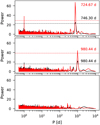 |
Fig. 2 Top panel: Lomb-Scargle (LS) periodogram of the RVs. The periodogram of the Lick data only is shown in black, while the LS periodogram of the complete RV dataset is shown in red. A RV offset and a jitter term are individually fitted for each dataset in addition to a global linear trend. The highest peak at ~ 735 ± 10 d is consistentwith the planet claimed by Wittenmyer et al. (2011). Center panel: LS periodogram of the residuals to the Keplerian orbit fit of the ~735 d signal. The highest peak at 980 d hints at the presence of a second planet in the system. Bottom panel: LS periodogram of the residuals to the Keplerian orbital fit of the two main signals. The horizontal lines in the panels show a false alarm probability level of 0.1% in black and red for Lick and complete dataset, respectively. The period of the highest peak in the LS periodogram is indicated with the color corresponding to each of the datasets. |
3.4 UCLES dataset
We included the RVs obtained between 2009 and 2011 and published by Wittenmyer et al. (2011) together with six more measurements presented in Wittenmyer et al. (2016). The 27 UCLES RVs were computed using the auSTRAL code (Endl et al. 2000), and have a mean internal velocity uncertainty of σUCLES ~ 1.5 ms−1.
4 Analysis
We computed a Lomb-Scargle (LS; Lomb 1976; Scargle 1982) periodogram to look for periodic signals in the RV data. Using the Lick data alone, we find a highly significant peak around 746 d, as shown in the top panel of Fig. 2. This result is consistentwith the already known planet of the system, for which Wittenmyer et al. (2011) announced a signal of 763 d. However, after fitting the reported planetary signal in our data, a significant peak around ~ 980 d is found in the residuals with false alarm probability smaller than 0.1% (see central panel of Fig. 2). After the fitting of these two periodic signals, no further signals are evident in the residuals, as shown in the bottom panel of Fig. 2. The weighted root mean square of the residuals improves from 12.9 ms−1 in the one-planet model fit to 8.2 ms−1 in the two-planet fit. The second signal could only be revealed thanks to the longer timespan of the Lick RVs compared to UCLES.
Following the second planet hint in the Lick data, we collected more observations with different facilities. The LS periodogram of the complete RV dataset shows narrower and stronger signals at the aforementioned periods, as shown in red in Fig. 2, further supporting the second planet hypothesis and constraining its orbital properties. The period of the second planet at 980 d is nearly in a 4:3 ratio with the first companion, suggesting a two-planet system likely in orbital resonance.
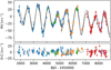 |
Fig. 3 Time series of the 182 RVs obtained for 7 CMa from September 2000 to April 2019 with Lick (blue), UCLES (orange), HARPS (before/after the fiber upgrade of 2015 in green/purple, respectively), and SONG (red) facilities. The vertical gray lines indicate the error bars including jitter. The best double Keplerian fit to the data is drawn with a dotted line, while the solid black line indicates the best dynamical two-planet fit. The residuals of the dynamical fit and the difference between the Keplerian and dynamical models (solid gray line) are shown in the bottom panel. |
4.1 Keplerian and dynamical modeling
We adopted a maximum-likelihood estimator coupled with a downhill simplex algorithm (Nelder & Mead 1965; Press et al. 1992) to determine the orbital parameters of the planet candidates orbiting 7 CMa. The negative logarithm of the likelihood function ( ) of the model is minimized while optimizing the planet orbital parameters, i.e., RV semi-amplitudes Kb,c, periods Pb,c, eccentricities eb,c, arguments of periastron ωb,c, mean anomalies Mb,c, and a RV zero-point offset for each dataset and a global RV slope. We also included the RV instrumental jitter as an additional model parameter for each dataset. Afterward, we estimate the uncertainties of the best-fit parameters using the Markov chain Monte Carlo (MCMC) sampler emcee (Foreman-Mackey et al. 2013). We adopted flat priors for all parameters and selected the 68.3 confidence interval levels of the posterior distributions as 1σ uncertainties. We used the EXO-STRIKER (Trifonov 2019) to perform all analyses discussed in this work.
First, we fit the RV dataset with a double-Keplerian model. The relatively close planetary orbits and the derived minimum masses of the planets indicate that the planets will have relatively close encounters during the time of the observations, which may be detected in our data. Therefore, a more appropriate N-body dynamical model is applied, which takes into account the gravitational interactions between the massive bodies by integrating the equations of motion using the Gragg-Bulirsch-Stoer method (Press et al. 1992). For consistency with the unperturbed Keplerian frame and in order to work with minimum dynamical masses, we assumed an edge-on and coplanar configuration for the 7 CMa system (i.e., ib,c = 90 deg and ΔΩ = 0 deg). The time step employed in the integration is 1 d.
Figure 3 shows the best-fit solutions from each of the schemes together with the complete RV dataset. The 7 CMa system contains two Jupiter-like planets with minimum masses mb sini ~ 1.8 MJ and mc sini ~ 0.9 MJ orbiting in low-eccentricity orbits. The period ratio of the planets in the 7 CMa system is close to 1.33, potentially trapped in a 4:3 MMR. The two models are almost equivalent and taking the gravitational interactions into account in the fitting does not turn into a significant improvement in the  of the fit with respect to the Keplerian model. The relatively short span of the observations (~ 9 orbits) is not enough to detect the secular perturbation of the orbits. However, although a double-Keplerian or a full self-consistent N-body dynamical model fit the RV data almost equally well, we decided to base our analysis on the dynamical model which, given the derived close orbits and the Jovian-like masses of the planets, is better justified. The orbital parameters of the two planets for the dynamical best fit and the posterior distributions from the MCMC sampling are summarized in Table 2.
We note that the jitter values derived for each dataset are all above 5 ms−1, as expected for K giants from p-mode oscillations (Hekker et al. 2006, 2008). Studying our high-cadence HARPS data we measured a peak-to-peak variation in the RVs of 5 ms−1 on timescales on the order of 30 min. From the scaling relations of Kjeldsen & Bedding (2011) we expected a velocity jitter of between 3 and 5 ms−1 for 7 CMa from p-mode oscillations, which is fully consistent with the derived jitter terms.
Orbital parameters of the 7 CMa system.
4.2 System configuration
The MCMC analysis provides a median solution that is in agreement with the best-fit solution except for the periods of both planets. Moreover, both solutions fail to preserve stability in a short period of time that is compatible with a handful of orbits of the outer planet. Thus, requiring long-term stability can further constrain the system configuration. The formally best-fit solution does not necessarily have to be stable, but we should find stable configurations close to the formally best-fit solution.
To test the stability of the planetary system around 7 CMa, we integrated each individual MCMC sample using the Wisdom-Holman symplectic algorithm (MVS) integrator contained in the SWIFT package (Duncan et al. 1998). This is a symplectic algorithm created to perform long-term numerical orbital integrations of solar system objects. All samples have been integrated for 1 Myr and the time step used for the integrations is 1 d to ensure accurate temporal resolution. A stable system is defined if none of the planets are ejected or experience a collision, the semimajor axes remain within 10% from the initial values, and the eccentricities are lower than 0.95 during the complete integration time; these values would otherwise lead to nonphysical orbits inside the radius of the star.
Figure 4 shows the posterior MCMC distribution of the orbital parameters using a dynamical, edge-on, coplanar model. The histogram panels on the top of Fig. 4 provide a comparison between the probability density function of the complete MCMC samples (blue) and the samples that are stable for at least 1 Myr (red) for each fitted parameter. The corner plot panels represent all possible parameter combinations with respect to the best dynamical fit from Table 2, whose position is denoted with a blue cross. The black 2D contours are constructed from the overall MCMC samples and indicate the 68.3, 95.5, and 99.7% confidence interval levels (i.e., 1σ, 2σ, and 3σ). For clarity, in Fig. 4 the stable samples are overplotted in red and the stable solution with the maximum  is indicated with a red cross.
We find that ~13% of the MCMC samples are stable. Moreover, the mode of the overall and stable samples are coincident for every orbital parameter and the best-fit stable solution is almost coincident with the median of the posteriors. Therefore, although the nominal best-fit solution ( ) derives a period for planets b and c that are off by 2σ from the mode of the samples, the actual configuration of the 7 CMa system is better represented by the stable best-fit solution (
 ) shown in the last column of Table 2.
In this stable configuration, the orbital periods of the planets are Pb ~ 737 d and Pc ~ 989 d, implying a period ratio of 1.34; while the nominal best-fit solution has a period ratio Pc ∕Pb = 1.22. This value is far from the 4:3 value that can preserve the stability of the system by trapping the planets in a 4:3 MMR, preventing the planets from close encounters. While the posterior distributions for the planet periods in the overall MCMC samples are very wide and asymmetrical, the periods of the stable samples are narrow and Gaussian-like, further supporting the validity of this solution despite its slightly lower statistical significance.
Furthermore, to describe the data correctly it is necessary to include a linear trend in the RV models. The RV slope is particularly evident in the Lick dataset and corresponds to ~ 1 ms−1 per year. A planet in a 50 yr period circular orbit assuming an RV semi-amplitude of about 12.5 ms−1 (which corresponds to the 1 ms−1 yr−1 trend over 25 yr) would have a minimum mass of 2 MJ. Increasing the period and semi-amplitude by a factor 2 the minimum mass would be 20 MJ. On the other hand, a three-planet fit to the data yields a  indistinguishable from a two-planet model and the period of the candidate is not well constrained. Although a third planet would not affect the stability of the inner pair, it could play an important role in the formation history of the system. Long-cadence observations of 7 CMa with the same instrumentation will shed light into the nature of the linear trend and possible further companions in the system.
Last, we tested the impact of coplanar inclined orbits (i.e., ib,c ≠90 deg, Ωb = Ωc = 0 deg) in the stability of the system. The impact of the inclinations with respect to the observer’s line of sight mainly manifests itself through the derived planetary masses, which are increased by a factor sin i. We chose a random subset of stable samples covering the parameter space of the red points in Fig. 4 and integrated these for 10 Myr with inclinations varying from 0 to 90 deg. We chose this simpler approach since a complete sampling of coplanar and mutually inclined systems (with ib, ic, Ωb, and Ωc as free parameters) in a dynamical fashion is computationally very expensive. Our analysis shows that these stable solutions cannot even preserve stability on very short timescales for ib = ic ≲ 70 deg. The larger planetary masses and higher interaction rate make these solutions much more fragile than the edge-on coplanar system.
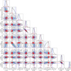 |
Fig. 4 Posterior distributions of the orbital parameters of the 7 CMa system. Each panel contains ~ 100 000 samples, which are tested for 1 Myr dynamical stability using the MVS integrator. Stable solutions are overplotted in red. The top panels of the corner plot show the probability density distributions of each orbital parameter of the overall MCMC samples (black) and the stable samples (red). The vertical dashed lines indicate the 16th, 50th, and the 84th percentiles of the overall MCMC samples. Contours are drawn to improve the visualization of the 2D histograms and indicate the 68.3, 95.5, and 99.7% confidence interval levels (i.e., 1σ, 2σ, and 3σ). Blue and red crosses indicate the dynamical best-fit solution (central column of Table 2) and the stable best-fit solution (last column of Table 2), respectively. |
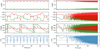 |
Fig. 5 Semimajor axes, eccentricities, resonant angles, and period-ratio evolution of one of the stable fits for 10 Myr. Planet b is shown in green, while planet c is in red. The left panel shows a 100 yr zoomed region of the complete 10 Myr simulation, shown in the right panel (we note the logarithmic scale in the X-axis). The system suffers from strong gravitational interactions on very short timescales, but it can preserve stability for 10 Myr. |
4.3 Dynamical properties
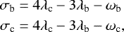
A period ratio close to 1.33 does not ensure that the system is indeed trapped in a 4:3 MMR. To test this scenario it is necessary to study thelong-term evolution of the orbital parameters and, particularly, the resonant angles. For the 4:3 MMR, these angles are defined as
 (1)
(1)
where the mean longitude λi = Mi + ωi (see, e.g., Murray & Dermott 1999).
Figure 5 shows the long-term evolution of an arbitrary stable sample chosen from the MCMC. This solution can preserve stability for at least 10 Myr, with semimajor axes and eccentricities oscillating rapidly with period ratios close to 1.33. The semimajor axes are strongly constrained to ab ~ 1.8 au and ac ~ 2.2 au, while the period-ratio of the planets oscillates slightly above the 4:3 value. The periodic drops in Pc ∕Pb are a consequence of the rapid variations in the semimajor axes when the two planets get close to each other.
The behavior of the resonant angles defines the location of the system with respect to the resonance: when one of the angles is librating, the system is said to be inside the resonance. The resonant angle of the first planet circulates from 0 deg to 360 deg, while σc is librating around 180 deg. The confinement of σc around 180 deg shows that it is the truly resonant librating angle of the 7 CMa system, as shown previously for the HD 200964 system by Tadeu dos Santos et al. (2015). Therefore, we can conclude that the two-planet system is effectively trapped in the narrow stable region of the 4:3 MMR and that the stability analysis reveals the true configuration of the system.
5 Conclusions
We report the discovery of a second planet orbiting the K-giant star 7 CMa. The extensive RV dataset reveals two massive Jupiter-like planets (mb sini ≈ 1.9 MJ, mc sini ≈ 0.9 MJ) orbiting closely in 4:3 MMR around their parent star. We find the true configuration of the system by studying the long-term stability of the planets since with the current data the periods are not well constrained. The mode of the MCMC samples is coincident with the median of the stable samples, which are narrow and Gaussian-like for all orbital parameters. The best nominal solution is within 2σ from the mode of the MCMC samples and with  with respect to the best stable fit.
The two-planet system around 7 CMa is the third to be discovered in 4:3 MMR, after HD 200964 (Johnson et al. 2011) and HD 5319 (Giguere et al. 2015). The existence of these massive planet systems challenge formation models since migration scales for passing through the 2:1 and 3:2 resonances are extremely short. This migration speed is almost impossible to achieve because a large amount of angular momentum should be delivered to the disk, as pointed out by Ogihara & Kobayashi (2013). Rein et al. (2012) reached the same conclusions using hydrodynamical simulations of convergent migration and in-situ formation. On the other hand, Tadeu dos Santos et al. (2015) were able to reproduce the formation process of HD 200964 using models that contained an interaction between the type I and type II of migration, planetary growth, and stellar evolution from the main sequence to the subgiant branch. However, the authors pointed out that the formation process is very sensitive to the planetary masses and protoplanetary disk parameters, where only a thin, vertically isothermal and laminar disk, with a nearly constant surface density profile allows the embryo-sized planets to reach the 4:3 resonant configuration. Another possible escape from the 2:1 and 3:2 resonances could be resonance overstability, as proposed by Goldreich & Schlichting (2014). In this case, convergent planetary migration with strongly damped eccentricities may only lead to a temporal capture at the 2:1 and 3:2 resonances. A detailed analysis on the formation of the 7 CMa system is out of the scope of this paper, but, given the similarities in the mass-ratio of the planets and the host star webelieve that this system could have undergone a similar formation and evolution as the HD 200964 system.
Acknowledgements
R.L. has received funding from the European Union’s Horizon 2020 research and innovation program under the Marie Skłodowska-Curie grant agreement No. 713673 and financial support through the “la Caixa” INPhINIT Fellowship Grant LCF/BQ/IN17/11620033 for Doctoral studies at Spanish Research Centres of Excellence from “la Caixa” Banking Foundation, Barcelona, Spain. S.R. and V.W. acknowledge support of the DFG priority program SPP 1992 “Exploring the Diversity of Extrasolar Planets” (RE 2694/5-1). M.H.L. was supported in part by Hong Kong RGC grant HKU 17305618. Based on observations made with the Hertzsprung SONG telescope operated on the Spanish Observatorio del Teide on the island of Tenerife by the Aarhus and Copenhagen Universities and by the Instituto de Astrofísica de Canarias.
References
- Andersen, M. F., Grundahl, F., Christensen-Dalsgaard, J., et al. 2014, Rev. Mex. Astron. Astrofis. Conf. Ser., 45, 83 [NASA ADS] [Google Scholar]
- Anglada-Escudé, G., López-Morales, M., & Chambers, J. E. 2010, ApJ, 709, 168 [NASA ADS] [CrossRef] [Google Scholar]
- Bailer-Jones, C. A. L., Rybizki, J., Fouesneau, M., Mantelet, G., & Andrae, R. 2018, AJ, 156, 58 [NASA ADS] [CrossRef] [Google Scholar]
- Ballard, S., & Johnson, J. A. 2016, ApJ, 816, 66 [NASA ADS] [CrossRef] [Google Scholar]
- Boisvert, J. H., Nelson, B. E., & Steffen, J. H. 2018, MNRAS, 480, 2846 [NASA ADS] [CrossRef] [Google Scholar]
- Bressan, A., Marigo, P., Girardi, L., et al. 2012, MNRAS, 427, 127 [NASA ADS] [CrossRef] [Google Scholar]
- Butler, R. P., Marcy, G. W., Williams, E., et al. 1996, PASP, 108, 500 [NASA ADS] [CrossRef] [Google Scholar]
- Ducati, J. R. 2002, VizieR Online Data Catalog: II/237 [Google Scholar]
- Duncan, M. J., Levison, H. F., & Lee, M. H. 1998, AJ, 116, 2067 [NASA ADS] [CrossRef] [EDP Sciences] [Google Scholar]
- Endl, M., Kürster, M., & Els, S. 2000, A&A, 362, 585 [Google Scholar]
- Foreman-Mackey, D., Hogg, D. W., Lang, D., & Goodman, J. 2013, PASP, 125, 306 [CrossRef] [Google Scholar]
- Frink, S., Quirrenbach, A., Fischer, D., Röser, S., & Schilbach, E. 2001, PASP, 113, 173 [NASA ADS] [CrossRef] [Google Scholar]
- Frink, S., Mitchell, D. S., Quirrenbach, A., et al. 2002, ApJ, 576, 478 [NASA ADS] [CrossRef] [MathSciNet] [Google Scholar]
- Gaia Collaboration (Brown, A. G. A., et al.) 2018, A&A, 616, A1 [NASA ADS] [CrossRef] [EDP Sciences] [Google Scholar]
- Giguere, M. J., Fischer, D. A., Payne, M. J., et al. 2015, ApJ, 799, 89 [NASA ADS] [CrossRef] [Google Scholar]
- Goldreich, P., & Schlichting, H. E. 2014, AJ, 147, 32 [NASA ADS] [CrossRef] [Google Scholar]
- Gray, R. O., Corbally, C. J., Garrison, R. F., et al. 2006, AJ, 132, 161 [NASA ADS] [CrossRef] [Google Scholar]
- Grundahl, F., Fredslund Andersen, M., Christensen-Dalsgaard, J., et al. 2017, ApJ, 836, 142 [NASA ADS] [CrossRef] [Google Scholar]
- Grundahl, F., Kjeldsen, H., Christensen-Dalsgaard, J., Arentoft, T., & Frandsen, S. 2007, Commun. Asteroseismol., 150, 300 [NASA ADS] [CrossRef] [Google Scholar]
- Hekker, S., & Meléndez, J. 2007, A&A, 475, 1003 [NASA ADS] [CrossRef] [EDP Sciences] [Google Scholar]
- Hekker, S., Reffert, S., Quirrenbach, A., et al. 2006, A&A, 454, 943 [NASA ADS] [CrossRef] [EDP Sciences] [Google Scholar]
- Hekker, S., Snellen, I. A. G., Aerts, C., et al. 2008, A&A, 480, 215 [NASA ADS] [CrossRef] [EDP Sciences] [Google Scholar]
- Johnson, J. A., Payne, M., Howard, A. W., et al. 2011, AJ, 141, 16 [NASA ADS] [CrossRef] [Google Scholar]
- Kjeldsen, H., & Bedding, T. R. 2011, A&A, 529, L8 [NASA ADS] [CrossRef] [EDP Sciences] [Google Scholar]
- Kürster, M., Trifonov, T., Reffert, S., Kostogryz, N. M., & Rodler, F. 2015, A&A, 577, A103 [NASA ADS] [CrossRef] [EDP Sciences] [Google Scholar]
- Lissauer, J. J., Ragozzine, D., Fabrycky, D. C., et al. 2011, ApJS, 197, 8 [NASA ADS] [CrossRef] [Google Scholar]
- Lo Curto, G., Pepe, F., Avila, G., et al. 2015, The Messenger, 162, 9 [NASA ADS] [Google Scholar]
- Lomb, N. R. 1976, Ap&SS, 39, 447 [NASA ADS] [CrossRef] [Google Scholar]
- Murray, C. D., & Dermott, S. F. 1999, Solar System Dynamics (Cambridge: Cambridge University Press) [Google Scholar]
- Nelder, J. A., & Mead, R. 1965, Comput. J., 7, 308 [Google Scholar]
- Ogihara, M., & Kobayashi, H. 2013, ApJ, 775, 34 [NASA ADS] [CrossRef] [Google Scholar]
- Piskunov, N. E., & Valenti, J. A. 2002, A&A, 385, 1095 [NASA ADS] [CrossRef] [EDP Sciences] [Google Scholar]
- Press, W. H., Teukolsky, S. A., Vetterling, W. T., & Flannery, B. P. 1992, Numerical Recipes in FORTRAN, the Art of Scientific Computing (New York: Cambridge University Press) [Google Scholar]
- Quirrenbach, A., Trifonov, T., Lee, M. H., & Reffert, S. 2019, A&A, 624, A18 [NASA ADS] [CrossRef] [EDP Sciences] [Google Scholar]
- Reffert, S., Quirrenbach, A., Mitchell, D. S., et al. 2006, ApJ, 652, 661 [NASA ADS] [CrossRef] [Google Scholar]
- Reffert, S., Bergmann, C., Quirrenbach, A., Trifonov, T., & Künstler, A. 2015, A&A, 574, A116 [NASA ADS] [CrossRef] [EDP Sciences] [Google Scholar]
- Rein, H., Payne, M. J., Veras, D., & Ford, E. B. 2012, MNRAS, 426, 187 [NASA ADS] [CrossRef] [Google Scholar]
- Ritter, A., Hyde, E. A., & Parker, Q. A. 2014, PASP, 126, 170 [NASA ADS] [CrossRef] [Google Scholar]
- Scargle, J. D. 1982, ApJ, 263, 835 [NASA ADS] [CrossRef] [Google Scholar]
- Schwab, C. 2010, PhD Thesis, University of Heidelberg, Germany [Google Scholar]
- Stock, S., Reffert, S., & Quirrenbach, A. 2018, A&A, 616, A33 [NASA ADS] [CrossRef] [EDP Sciences] [Google Scholar]
- Tadeu dos Santos, M., Correa-Otto, J. A., Michtchenko, T. A., & Ferraz-Mello, S. 2015, A&A, 573, A94 [NASA ADS] [CrossRef] [EDP Sciences] [Google Scholar]
- Trifonov, T. 2019, Astrophysics Source Code Library [record ascl:1906.004] [Google Scholar]
- Trifonov, T., Reffert, S., Tan, X., Lee, M. H., & Quirrenbach, A. 2014, A&A, 568, A64 [NASA ADS] [CrossRef] [EDP Sciences] [Google Scholar]
- Trifonov, T., Reffert, S., Zechmeister, M., Reiners, A., & Quirrenbach, A. 2015, A&A, 582, A54 [NASA ADS] [CrossRef] [EDP Sciences] [Google Scholar]
- Trifonov, T., Stock, S., Henning, T., et al. 2019, AJ, 157, 93 [NASA ADS] [CrossRef] [Google Scholar]
- van Leeuwen, F. 2007, A&A, 474, 653 [NASA ADS] [CrossRef] [EDP Sciences] [Google Scholar]
- Wittenmyer, R. A., Endl, M., Wang, L., et al. 2011, ApJ, 743, 184 [NASA ADS] [CrossRef] [Google Scholar]
- Wittenmyer, R. A., Butler, R. P., Wang, L., et al. 2016, MNRAS, 455, 1398 [NASA ADS] [CrossRef] [Google Scholar]
- Wittenmyer, R. A., Bergmann, C., Horner, J., Clark, J., & Kane, S. R. 2019, MNRAS, 484, 4230 [NASA ADS] [CrossRef] [Google Scholar]
- Zechmeister, M., Reiners, A., Amado, P. J., et al. 2018, A&A, 609, A12 [CrossRef] [Google Scholar]
All Tables
All Figures
|
Fig. 1 Interpolated evolutionary track for 7 CMa in the Hertzsprung–Russell diagram. The different evolutionary phases are color-coded. The sluminosity and temperature of the star, including uncertainties, are shown in black. |
| In the text | |
|
Fig. 2 Top panel: Lomb-Scargle (LS) periodogram of the RVs. The periodogram of the Lick data only is shown in black, while the LS periodogram of the complete RV dataset is shown in red. A RV offset and a jitter term are individually fitted for each dataset in addition to a global linear trend. The highest peak at ~ 735 ± 10 d is consistentwith the planet claimed by Wittenmyer et al. (2011). Center panel: LS periodogram of the residuals to the Keplerian orbit fit of the ~735 d signal. The highest peak at 980 d hints at the presence of a second planet in the system. Bottom panel: LS periodogram of the residuals to the Keplerian orbital fit of the two main signals. The horizontal lines in the panels show a false alarm probability level of 0.1% in black and red for Lick and complete dataset, respectively. The period of the highest peak in the LS periodogram is indicated with the color corresponding to each of the datasets. |
| In the text | |
|
Fig. 3 Time series of the 182 RVs obtained for 7 CMa from September 2000 to April 2019 with Lick (blue), UCLES (orange), HARPS (before/after the fiber upgrade of 2015 in green/purple, respectively), and SONG (red) facilities. The vertical gray lines indicate the error bars including jitter. The best double Keplerian fit to the data is drawn with a dotted line, while the solid black line indicates the best dynamical two-planet fit. The residuals of the dynamical fit and the difference between the Keplerian and dynamical models (solid gray line) are shown in the bottom panel. |
| In the text | |
|
Fig. 4 Posterior distributions of the orbital parameters of the 7 CMa system. Each panel contains ~ 100 000 samples, which are tested for 1 Myr dynamical stability using the MVS integrator. Stable solutions are overplotted in red. The top panels of the corner plot show the probability density distributions of each orbital parameter of the overall MCMC samples (black) and the stable samples (red). The vertical dashed lines indicate the 16th, 50th, and the 84th percentiles of the overall MCMC samples. Contours are drawn to improve the visualization of the 2D histograms and indicate the 68.3, 95.5, and 99.7% confidence interval levels (i.e., 1σ, 2σ, and 3σ). Blue and red crosses indicate the dynamical best-fit solution (central column of Table 2) and the stable best-fit solution (last column of Table 2), respectively. |
| In the text | |
|
Fig. 5 Semimajor axes, eccentricities, resonant angles, and period-ratio evolution of one of the stable fits for 10 Myr. Planet b is shown in green, while planet c is in red. The left panel shows a 100 yr zoomed region of the complete 10 Myr simulation, shown in the right panel (we note the logarithmic scale in the X-axis). The system suffers from strong gravitational interactions on very short timescales, but it can preserve stability for 10 Myr. |
| In the text | |
Current usage metrics show cumulative count of Article Views (full-text article views including HTML views, PDF and ePub downloads, according to the available data) and Abstracts Views on Vision4Press platform.
Data correspond to usage on the plateform after 2015. The current usage metrics is available 48-96 hours after online publication and is updated daily on week days.
Initial download of the metrics may take a while.