| Issue |
A&A
Volume 631, November 2019
|
|
|---|---|---|
| Article Number | A119 | |
| Number of page(s) | 21 | |
| Section | Astronomical instrumentation | |
| DOI | https://doi.org/10.1051/0004-6361/201936405 | |
| Published online | 05 November 2019 | |
J-PLUS: photometric calibration of large-area multi-filter surveys with stellar and white dwarf loci
1
Centro de Estudios de Física del Cosmos de Aragón, Unidad Asociada al CSIC, Plaza San Juan 1, 44001 Teruel, Spain
e-mail: clsj@cefca.es
2
Institut de Ciències del Cosmos, Universitat de Barcelona (IEEC-UB), Martí i Franquès 1, 08028 Barcelona, Spain
3
Department of Physics, University of Warwick, Coventry CV4 7AL, UK
4
Department of Physics and JINA Center for the Evolution of the Elements, University of Notre Dame, Notre Dame, IN 46556, USA
5
Instituto de Astronomia, Geofísica e Ciências Atmosféricas, Universidade de São Paulo, 05508-090 São Paulo, Brazil
6
IAA-CSIC, Glorieta de la Astronomía s/n, 18008 Granada, Spain
7
Centro de Astrobiología (CSIC-INTA), ESAC Campus, Camino Bajo del Castillo s/n, 28692 Villanueva de la Cañada, Spain
8
Spanish Virtual Observatory, 28692 Villanueva de la Cañada, Spain
9
Observatório Nacional, Rua General José Cristino, 77 – Bairro Imperial de São Cristóvão, 20921-400 Rio de Janeiro, Brazil
10
Department of Physics, Lancaster University, Lancaster LA1 4YB, UK
11
Leiden Observatory, Leiden University, PO Box 9513 2300, RA Leiden, The Netherlands
12
Donostia International Physics Centre (DIPC), Paseo Manuel de Lardizabal 4, 20018 Donostia-San Sebastián, Spain
13
IKERBASQUE, Basque Foundation for Science, 48013 Bilbao, Spain
14
University of Michigan, Department of Astronomy, 1085 South University Ave., Ann Arbor, MI 48109, USA
15
University of Alabama, Department of Physics and Astronomy, Gallalee Hall, Tuscaloosa, AL 35401, USA
Received:
30
July
2019
Accepted:
5
September
2019
Aims. We present the photometric calibration of the 12 optical passbands observed by the Javalambre Photometric Local Universe Survey (J-PLUS).
Methods. The proposed calibration method has four steps: (i) definition of a high-quality set of calibration stars using Gaia information and available 3D dust maps; (ii) anchoring of the J-PLUS gri passbands to the Pan-STARRS photometric solution, accounting for the variation in the calibration with the position of the sources on the CCD; (iii) homogenization of the photometry in the other nine J-PLUS filters using the dust de-reddened instrumental stellar locus in (𝒳 − r) versus (g − i) colours, where 𝒳 is the filter to calibrate. The zero point variation along the CCD in these filters was estimated with the distance to the stellar locus. Finally, (iv) the absolute colour calibration was obtained with the white dwarf locus. We performed a joint Bayesian modelling of 11 J-PLUS colour–colour diagrams using the theoretical white dwarf locus as reference. This provides the needed offsets to transform instrumental magnitudes to calibrated magnitudes outside the atmosphere.
Results. The uncertainty of the J-PLUS photometric calibration, estimated from duplicated objects observed in adjacent pointings and accounting for the absolute colour and flux calibration errors, are ∼19 mmag in u, J0378, and J0395; ∼11 mmag in J0410 and J0430; and ∼8 mmag in g, J0515, r, J0660, i, J0861, and z.
Conclusions. We present an optimized calibration method for the large-area multi-filter J-PLUS project, reaching 1–2% accuracy within an area of 1022 square degrees without the need for long observing calibration campaigns or constant atmospheric monitoring. The proposed method will be adapted for the photometric calibration of J-PAS, that will observe several thousand square degrees with 56 narrow optical filters.
Key words: methods: statistical / techniques: photometric
© ESO 2019
1. Introduction
The analysis of Milky Way (MW) stars and the understanding of extragalactic sources have greatly benefited from large (≳5000 deg2) and systematic optical and near-infrared photometric surveys, such as the second Palomar Observatory Sky Survey (POSS-II; Gal et al. 2004), the Sloan Digital Sky Survey (SDSS; Abazajian et al. 2009), the Two Micron All-Sky Survey (2MASS; Skrutskie et al. 2006), or the VISTA Hemisphere Survey (VHS; McMahon et al. 2013). These studies will move forward in the following decade with several on-going and planned next-generation surveys, some of them summarized in Table 1 for reference.
Compilation of finished (F), on-going (O), and scheduled (S) optical and near-infrared large-area (≳5000 deg2) photometric surveys.
One fundamental step in the data processing of all the major surveys is the photometric calibration of the observations. The calibration process aims to translate the observed counts in astronomical images to a physical flux scale referred to the top of the atmosphere. Because accurate colours are needed to derive photometric redshifts for galaxies and atmospheric parameters for stars, and reliable absolute fluxes are involved in the estimation of the luminosity and the stellar mass of galaxies, current and future photometric surveys target a calibration uncertainty at the 1% level and below to reach their ambitious scientific goals.
The traditional calibration approach relies in a network of standard stars with a well-known flux across the wavelength range of interest. The monitoring of these standards with the survey photometric system permits us to calibrate the observations. The calibration of large-area multi-filter surveys has two main challenges that are not optimally tackled with this traditional method: obtaining a homogeneous photometric calibration across areas of thousands of square degrees and performing a consistent wavelength calibration for dozens of passbands.
Thanks to lessons learnt from SDSS, the repeated scan of calibration fields, and the constant monitoring of the sky conditions, methodologies such as ubercalibration, supercalibration, and hypercalibration; the estimation of photometric flat fields; or the forward photometric modelling have been successfully applied to reach 1% level precision in broad-band surveys (Padmanabhan et al. 2008; Regnault et al. 2009; Wittman et al. 2012; Schlafly et al. 2012; Ofek et al. 2012; Burke et al. 2014, 2018; Scolnic et al. 2015; Magnier et al. 2016b; Finkbeiner et al. 2016; Zhou et al. 2018). These methodologies were envisioned to provide homogeneous calibration over large areas and can also be applied to multi-filter surveys, but the large number of passbands makes the calibration campaigns extremely time consuming and the calibration observations can take as long as the scientific operations. To optimize the telescope time and speed up the survey progress, novel calibration strategies must be developed for projects such as the Javalambre Photometric Local Universe Survey (J-PLUS1; Cenarro et al. 2019), the Southern Photometric Local Universe Survey (S-PLUS; Mendes de Oliveira et al. 2019), and the Javalambre Physics of the accelerating universe Astrophysical Survey (J-PAS2; Benítez et al. 2014).
The present paper summarizes the efforts in the quest for an optimized photometric calibration procedure for J-PLUS. The survey started in November 2015, and over the last four years several calibration methods have been implemented and tested. The growing amount of data, the improved knowledge of the telescope optics and the filter system, and the efforts of the community to produce other high-quality legacy datasets (Table 1) have permitted the fine tuning of the calibration method to achieve the goal of 1% precision in most of the J-PLUS filters. As reference, we provide a brief description of the previous calibration procedures applied to J-PLUS data in Sect. 3, and the instructions to update public J-PLUS photometry with the new calibration method presented in this work in Sect. 6.
This paper is organized as follows. In Sect. 2 we present the J-PLUS data and the ancillary datasets used in the calibration process. A summary of the previous calibration methods is presented in Sect. 3. The current concordance photometric calibration methodology is detailed in Sect. 4, and the calibration precision is presented in Sect. 5. The recipes used to apply the new calibration to J-PLUS data are outlined in Sect. 6. We present our conclusions in Sect. 7. Magnitudes are given in the AB system (Oke & Gunn 1983).
2. J-PLUS photometric data
J-PLUS is a photometric survey of several thousand square degrees that is being conducted from the Observatorio Astrofísico de Javalambre (OAJ, Teruel, Spain; Cenarro et al. 2014) using the 83 cm Javalambre Auxiliary Survey Telescope (JAST/T80) and the T80Cam, a panoramic camera of 9.2k × 9.2k pixels that provides a 2deg2 field of view (FoV) with a pixel scale of 0.55″ pix−1 (Marín-Franch et al. 2015). The J-PLUS filter system, composed of 12 bands, is summarized in Table 2. The J-PLUS observational strategy, image reduction, and main scientific goals are presented in Cenarro et al. (2019).
J-PLUS photometric system, extinction coefficients, and limiting magnitudes (5σ, 3″ aperture) of J-PLUS DR1 (Cenarro et al. 2019).
The J-PLUS first data release (DR1) comprises 511 pointings (1022 deg2) observed and reduced in 12 optical filters (Cenarro et al. 2019). The limiting magnitudes (5σ, 3″ aperture) of the DR1 are presented in Table 2 for reference. The median point spread function (PSF) full width at half maximum (FWHM) in the DR1 r-band images is 1.1″. Source detection was done in the r band using SExtractor (Bertin & Arnouts 1996), and the flux measured in the 12 J-PLUS bands at the position of the detected sources using the aperture defined in the r-band image. Objects near the borders of the images, close to bright stars, or affected by optical artefacts were masked. The DR1 is publicly available at the J-PLUS website3.
The new calibration process presented in Sect. 4 uses J-PLUS DR1 in combination with ancillary data from Gaia and the Panoramic Survey Telescope and Rapid Response System (Pan-STARRS), so we describe these datasets in the following.
2.1. Pan-STARRS DR1
The Pan-STARRS 1 is a 1.8 m optical and near-infrared telescope located on Mount Haleakala, Hawaii. The telescope is equipped with the Gigapixel Camera 1 (GPC1), consisting of an array of 60 CCD detectors, each 4800 pixels on a side (Chambers et al. 2016).
The 3π Stereoradian Survey (hereafter PS1; Chambers et al. 2016) covers the sky north of declination δ = −30° in four SDSS-like passbands, griz, with an additional passband in the near-infrared, y. The entire filter set spans the range 400 − 1000 nm (Tonry et al. 2012).
Astrometry and photometry were extracted by the Pan-STARRS 1 Image Processing Pipeline (Magnier et al. 2016a,b,c; Waters et al. 2016). PS1 photometry features a uniform flux calibration, achieving better than 1% precision over the sky (Magnier et al. 2016b; Chambers et al. 2016). In single-epoch photometry, PS1 reaches typical 5σ depths of 22.0, 21.8, 21.5, 20.9, and 19.7 in grizy, respectively (Chambers et al. 2016). The PS1 DR1 occurred in December 2016, and provided a static-sky catalogue, stacked images from the 3π Stereoradian Survey, and other data products (Flewelling et al. 2016).
Because of its large footprint, homogeneous depth, and excellent internal calibration, PS1 photometry provides an ideal reference for the calibration of the gri J-PLUS broad bands.
2.2. Gaia DR2
The Gaia spacecraft is mapping the 3D positions and kinematics of a representative fraction of MW stars (Gaia Collaboration 2016). The mission will eventually provide astrometry (positions, proper motions, and parallaxes) and optical spectrophotometry for over a billion stars, as well as radial velocity measurements of more than 100 million stars.
In the present paper we used the Gaia DR2 (Gaia Collaboration 2018a). It contains five-parameter astrometric determinations and provides integrated photometry in three broad bands, G, GBP (330 − 680 nm), and GRP (630 − 10501 nm), for 1.4 billion sources with G < 21. The typical uncertainties in Gaia DR2 measurements at G = 17 are ∼0.1 marcsec in parallax, ∼2 mmag in G-band photometry, and ∼10 mmag in GBP and GRP magnitudes (Gaia Collaboration 2018a).
3. Previous calibration methods applied to J-PLUS data
The different procedures implemented to perform the photometric calibration of the J-PLUS DR1 observations have provided precious knowledge regarding the optimized method presented in Sect. 4. Thus, a proper presentation of these methods is mandatory to understand the strengths and weaknesses of each procedure, and motivates the need for a new methodology.
The ultimate goal of any calibration strategy is to obtain the zero point (ZP) of the observation, that relates the magnitude of the sources in passband 𝒳 on top of the atmosphere with the magnitudes obtained from the analogue to digital unit (ADU) counts of the reduced images. We simplify the notation in the following using the passband name as the magnitude in such filter. Thus,

In the estimation of the J-PLUS DR1 raw catalogues, the reduced images were normalized to a one-second exposure and ZP𝒳 = 25 was used. This defined the instrumental magnitudes 𝒳ins.
3.1. Spectro-photometric standard stars
The main sources for the spectro-photometric standard stars (SSSs) are the spectral libraries CALSPEC4, the Next Generation Spectral Library5, and STELIB (Le Borgne et al. 2003). Following the calibration procedure based on Bouguer fitting lines, each SSS is observed at different airmasses throughout the night to derive the atmospheric extinction coefficient and the photometric zero point of the system. The synthetic magnitudes of the SSSs were estimated by convolving the reference spectra with the J-PLUS photometric system, and the instrumental magnitudes were estimated from the Moffat (1969) profile fitting to the observed light distribution of the SSSs. For this procedure to be accurate, the atmospheric conditions must be stable throughout the night.
Strengths. Consistent absolute flux calibration of the 12 J-PLUS filters.
Weaknesses. The calibration observations consume a significant fraction of telescope time. The typical magnitudes of the SSSs can produce saturated images in the broad bands. It can only be applied during full photometric nights.
3.2. Comparison with broad-band photometry
The significant overlap (∼80%) between J-PLUS and SDSS footprints allows calibration of the J-PLUS broad-band observations against the corresponding ones in SDSS. This technique was used to calibrate the ugriz bands by comparing J-PLUS 6″ aperture instrumental magnitudes and SDSS PSF magnitudes. Because of differences in the effective transmission curves between SDSS and J-PLUS photometric systems, colour-term corrections need to be applied to the SDSS magnitudes to obtain the corresponding J-PLUS photometry. These corrections are of particular importance in the case of the u band, where filters are known to be significantly different.
The same procedure was applied using PS1 photometry as reference. In this case, any J-PLUS observation is covered by PS1, but only the griz bands are available. The colour-term corrections are significant in the case of the g band.
Strengths. Reliable and accurate flux calibration of the J-PLUS broad bands. High density of sources used to perform the calibration. Can also be applied during non-photometric nights.
Weaknesses. The calibration of the seven J-PLUS medium bands is missing. Only a fraction of the J-PLUS area is covered by SDSS, while we have no access to the u band with PS1. We inherit any flux calibration bias affecting the reference photometry (see Lorenzo-Gutiérrez et al. 2019, for caveats about SDSS photometry at g ≲ 15).
3.3. Comparison with SDSS spectroscopy
This method starts by convolving the SDSS stellar spectra with the spectral response for each J-PLUS passband, yielding synthetic magnitudes. A comparison to the observed magnitudes in 6″ aperture provides estimates for the zero points. Although the sky coverage of the SDSS spectra is smaller and sparser than J-PLUS photometry, it can be used to calibrate those J-PLUS passbands that have no photometric counterpart. In particular, given the spectral coverage of the SDSS spectra, they are used to calibrate the J-PLUS passbands from J0395 to J0861, including gri broad bands. With the installation of the BOSS spectrograph (Smee et al. 2013), the wavelength range of the spectra was extended to the blue, thus allowing the calibration of the J0378 band in areas of the sky for which BOSS spectra are available. However, u and z bands still fall outside of the range covered by SDSS spectroscopy. Given the wide FoV of T80Cam at JAST/T80, dozens of high-quality SDSS stellar spectra in a single J-PLUS pointing are frequent.
Strengths. Consistent flux calibration of the medium-band J-PLUS filters. Can be applied during non-photometric nights.
Weaknesses. The calibration of u and z is missing. SDSS spectroscopy does not cover all of the J-PLUS area. Source density is low with respect to the photometric case. We inherit any flux calibration bias affecting SDSS spectra.
3.4. Stellar locus regression
The previous procedures were designed to be applied to any single exposure or any combination of exposures in a given filter, independently of the observations in any other band. However, by combining the information from different bands, it is possible to apply methods that enable anchoring the calibration throughout the spectral range. One particular approach is the use of the stellar locus (Covey et al. 2007; High et al. 2009; Kelly et al. 2014; Kuijken et al. 2019). This procedure takes advantage of the way stars with different stellar parameters populate colour–colour diagrams, defining a well-constrained region (stellar locus) whose shape depends on the specific colours used.
The implemented stellar locus regression (SLR) first constructs the median stellar locus in all the 2145 possible colour–colour combinations in J-PLUS. The initial photometry used to estimate the median locus relies on the previous calibration procedures: SDSS photometry for u and z, and SDSS spectroscopy for the rest of the J-PLUS passbands. The SLR works with relative colours, so a reference filter is needed. In this case, the i band provided the best results and was anchored to the available broad-band photometric reference: SDSS or PS1 in those pointings outside the SDSS footprint. Then the distance of the 2145 stellar loci in each pointing to the median loci was minimized in an iterative process, leading to 11 offsets per pointing.
Strengths. Consistent relative flux calibration of the 12 J-PLUS filters in all of the surveyed area. Can be applied during non-photometric nights.
Weaknesses. Needs a minimum density of stars to populate the stellar locus. Cannot be used for stand-alone calibration of one image. Needs at least one reference band with external calibration. The current version does not include the effect of MW dust reddening in the estimation of the median stellar locus.
3.5. Summary
A detailed description of the previous methods can be found in Varela & Cristóbal-Hornillos (2017). The tests performed reveal that the best current option is the SLR, because it provides a consistent calibration in all the J-PLUS filters, pointings, and atmospheric conditions. The SLR has therefore been the reference calibration method in J-PLUS DR1, and all the available calibrations for a given filter and pointing are accessible in the J-PLUS database, ADQL table jplus.CalibTileImage.
The SLR calibration in J-PLUS DR1 has two main drawbacks. First, the Milky Way extinction is not accounted for in the stellar locus estimation. This implies that inhomogeneities in the survey photometry due to differential dust reddening are absorbed by the zero points, and therefore the calibration does not refer to the top of the atmosphere but to some intermediate location of the MW halo. This complicates the interpretation of the data and the proper de-reddening of J-PLUS magnitudes for galactic and extragalactic studies. Second, the data used to estimate the reference stellar locus relies on other calibration methods, and thus the SLR inherits any flux bias from the primary calibration source. These two issues lead us to define the new concordance methodology described in the next section.
4. J-PLUS photometric calibration with stellar and white dwarf loci
In this section we provide the details of the proposed methodology for the photometric calibration of the multi-filter J-PLUS project. We started by gathering the needed information to define a high-quality set of stars for calibration (Sect. 4.1). Then, we anchored the J-PLUS photometry in the gri broad bands to the PS1 photometry (Sect. 4.2). Next, we homogenized the photometric solution along the J-PLUS area in the other nine passbands with the instrumental stellar locus (Sect. 4.3). Finally, we estimated the absolute colour calibration of the J-PLUS passbands with the white dwarf locus (Sect. 4.4). The performance and the error budget of the obtained photometric calibration are presented in Sect. 5. A flowchart of the calibration process is presented in Fig. 1.
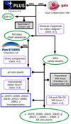 |
Fig. 1. Flowchart of the calibration method presented in this work. Arrows that originate in small dots indicate that the preceding data product is an input to the subsequent analysis. Datasets are shown with their project logo, and external codes or models with grey boxes. The rounded-shape boxes show the calibration steps. The asterisks indicate those steps based on dust de-reddened magnitudes. The white boxes show intermediate data products, and ovals highlight publicly available data products of the calibration process. |
The strengths of the new method are that it permits a consistent flux calibration of the 12 J-PLUS filters in all the surveyed area, it can be applied during non-photometric nights, no previous calibration of the medium bands is needed, and it includes the effect of MW dust in the stellar locus estimation. The weaknesses are similar to those of SLR, mainly a minimum density of stars to populate the stellar and white dwarf loci, and one reference band with external absolute calibration are needed. The former issue is circumvented thanks to the wide FoV of T80Cam at JAST/T80, which always provides a few hundred high-quality stars for calibration, and to the large area already covered by J-PLUS DR1, which provides enough numbers of the sparse white dwarfs to take advantage of their locus. The latter issue is mitigated thanks to the excellent external photometric reference provided by PS1 in the gri passbands.
The J-PLUS instrumental magnitudes used for calibration were measured in a 6″ diameter aperture. This aperture ensures a low flux contamination from neighbouring sources and is not dominated by background noise, but it is not large enough to capture the total flux of the stars. Thus, we applied an aperture correction Caper that depends on the pointing and the passband. The aperture correction was computed from the growth curves of bright, non-saturated stars in the pointing. The typical number of stars used is 50 and the median aperture correction varies from Caper = −0.09 mag in the u band to Caper = −0.11 mag in the z band, with a median value of Caper = −0.1 mag for all the filters. We assumed that the J-PLUS 6″ magnitudes corrected for aperture effects provided the total flux of stars.
4.1. Step 1: definition of the high-quality stellar set for calibration
The initial stage of our methodology aims to define the high-quality sample of stars needed to perform the photometric calibration. We started by cross-matching the J-PLUS sources with signal-to-noise S/N > 10 and SExtractor photometric flag equal to zero (i.e. with neither close detections nor image problems) in all 12 passbands against the Gaia DR2 catalogue using a 1.5″ radius6. We discarded those J-PLUS sources with more than one Gaia counterpart, and those with either S/N < 3 in Gaia parallax, noted ϖ [arcsec], or without a photometric measurement in any G, GBP, or GRP passband. We obtained 496 798 unique high-quality stars for calibration.
We applied the correction to the G photometry and the Vega to AB conversions presented in Maíz Apellániz & Weiler (2018). The median G magnitude of the calibration sample is G = 15.7 mag, with 99% of the sources having G ≲ 17.5 mag.
We worked with dust de-reddened magnitudes and colours in several stages of the calibration process. We computed the extinction coefficients k𝒳 of each J-PLUS passband using the extinction law presented in Schlafly et al. (2016, hereafter S16)7. These coefficients, presented in Table 2, assume RV = 3.1. The de-reddened J-PLUS photometry, either instrumental or calibrated, is noted with the subscript 0 and was obtained as

We estimated the colour excess E(B − V) [mag] of each J-PLUS + Gaia matched source from the 3D dust maps provided by Bayestar178 (Green et al. 2018). As stated by the authors, the colour excess EB17 retrieved by Bayestar17 is not directly E(B − V), so we scaled the output from Bayestar17 to ensure the same (r − i) colour excess both in J-PLUS and PS1. This implies E(B − V) = 0.92 × EB17 (see Green et al. 2018 for further details). We study the impact of the assumed extinction law in our results in Sect. 5.5.
The parallax measured by Gaia can be used to estimate the distance to the calibration stars. As discussed in Luri et al. (2018) and Bailer-Jones et al. (2018), this estimation should account for the inherent asymmetry in the parallax to distance transformation. To properly account for the uncertainties in the 3D dust maps and in the distances estimated from Gaia parallaxes, we extracted 10 000 random points ϖrand from a Gaussian distribution ϖ ± σϖ in the parallax of each source. Then we imposed a positive parallax value and computed the attenuation at the corresponding distance, drand = 1/ϖrand, and sky position of the source using each time a random dust map solution from Bayestar17. Then the median and the ±34% of the attenuation distribution were recorded as the value of the colour excess E(B − V) and its error. We checked that the colour excess distribution is Gaussian in most cases, providing a proper description of E(B − V) for each calibration star. This procedure naturally accounts for the asymmetry in the distances and applies a d > 0 prior (i.e. no Galaxy model has been assumed in the computation of the distances; see Luri et al. 2018 and Bailer-Jones et al. 2018 for an extensive discussion). We find that 99% of the high-quality sources have E(B − V) < 0.14 mag, with a typical error in the estimated colour excess of σE(B − V) ∼ 0.006 mag.
The extinction coefficients of G, GBP, and GRP were obtained as for the J-PLUS passbands: kG = 2.600, kGBP = 3.410, and kGRP = 1.807. This provides first-order de-reddened magnitudes and colours, since the proper extinction correction of Gaia photometry is colour and dust-column dependent (Danielski et al. 2018; Gaia Collaboration 2018b). However, the low extinction at the J-PLUS pointings makes this simple correction sufficient for our goal, i.e. to define a sample of calibration stars.
We estimated the G-band absolute magnitude of the J-PLUS + Gaia sources as

This estimation assumes a dust de-reddening using the Bayestar17 colour excess with the simplified extinction coefficients mentioned above, and the inverse of the parallax as a distance proxy. We note that the latter is a crude approximation to the Bayesian distance provided by Bailer-Jones et al. (2018). Because we aim to define general populations to calibrate the J-PLUS photometry, all these simplifications fulfil our requirements.
The absolute magnitude–colour diagram of the J-PLUS + Gaia sample of high-quality stars is presented in Fig. 2. We selected three populations on this diagram, named main sequence (MS) stars, giant branch (GB) stars, and white dwarfs (WDs). Formally,
![$$ \begin{aligned}&\mathrm{WD} = [\,M_{G_0} > 7\,]\ \cap \ [\,(G_{\rm BP} - G_{\rm RP})_0 < 0.35\,] \cap \nonumber \\&\qquad \quad [\,M_{G_0} > 10.5 + 7\times (G_{\rm BP} - G_{\rm RP})_0\,], \end{aligned} $$](/articles/aa/full_html/2019/11/aa36405-19/aa36405-19-eq6.gif)
![$$ \begin{aligned}&\mathrm{GB} = [\,M_{G_0} < 4.1\,]\ \cap \ [\,(G_{\rm BP} - G_{\rm RP})_0 > 0.35\,] \cap \nonumber \\&\qquad \quad [\,M_{G_0} < -1.5 + 8\times (G_{\rm BP} - G_{\rm RP})_0\,], \end{aligned} $$](/articles/aa/full_html/2019/11/aa36405-19/aa36405-19-eq7.gif)
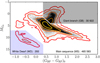 |
Fig. 2. Absolute magnitude in the G band vs. GBP − GRP colour diagram, corrected for dust reddening, of the 496 798 high-quality sources in common between J-PLUS DR1 and Gaia DR2. The black dots are individual measurements. The coloured solid contours show density of objects, starting on 25 mag−2 and increasing by a factor of ten in each step. We define three populations on this diagram: main sequence stars (465 583; white area), giant branch stars (30 922; grey area), and white dwarfs (293; blue area). |
and
where the superindex c denotes the absolute complement set. These broad classes can contain other types of objects, such as hot sub-dwarfs or unresolved binaries in the case of the main sequence area. We note that main sequence and giant branch stars could have been used together in the next calibration steps, but we preferred to split them to minimize secondary branches in those colour–colour diagrams that include J-PLUS filters sensitive to gravity (i.e. J0515).
We obtained 465 583 main sequence stars (94% of the total sample), 30 922 giant branch stars (6%), and 293 white dwarfs (< 0.1%). The median distances to these populations are dMS = 1.4 kpc, dGB = 3.0 kpc, and dWD = 0.2 kpc, while the median colour excesses are E(B − V)MS = 0.041 mag, E(B − V)GB = 0.047 mag, and E(B − V)WD = 0.016 mag. The colour excess distribution9 of the three populations is presented in Fig. 3. The main sequence stars were used to homogenize the photometry in the full J-PLUS area (Sects. 4.2 and 4.3), the giant branch stars to test the calibration procedure (Sect. 5.2), and the white dwarf locus to provide an absolute calibration of the J-PLUS colours (Sect. 4.4).
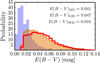 |
Fig. 3. Probability distribution of the colour excess E(B − V) for the three populations defined in the absolute magnitude vs. colour diagram: main sequence stars (MS, orange hatched histogram), giant branch stars (GB, red histogram), and white dwarfs (WD, blue filled histogram). The median colour excess of each population is labelled in the panel. |
4.2. Step 2: anchoring gri broad bands with PS1 data
The next step in our calibration process aims to anchor the J-PLUS photometry to the PS1 photometric solution in the shared gri broad-band filters. The PS1 photometry is currently the reference of other broad-band photometric surveys such as SDSS (Finkbeiner et al. 2016), the Dark Energy Spectroscopic Instrument (DESI) Legacy Surveys (Dey et al. 2019), or the Hyper Suprime-Cam Subaru Strategic Program (HSC, Aihara et al. 2019). Moreover, PS1 observations cover all the sky visible from OAJ, providing a consistent reference for any J-PLUS observation.
We cross-matched our MS calibration set with the PS1 DR1 catalogue using a 1.5″ radius10. As in the Gaia case, we discarded those sources with more than one counterpart in the PS1 catalogue or without a photometric measurement in any PS1 passband. We used the PS1 PSF magnitudes as reference. As stated by Magnier et al. (2016c), the PSF magnitudes in PS1 were optimized to minimize the difference with respect to aperture-corrected magnitudes, and thus are a good proxy for the total flux of stars.
To account for the differences between the J-PLUS and PS1 photometric systems, we applied the following transformation equations, T𝒳 = 𝒳PS1 − 𝒳J − PLUS, where 𝒳 is the passband under study
![$$ \begin{aligned}&T_g = 0.8 - 88.6 \times \mathcal{C} _{\rm PS1} + 22.5 \times \mathcal{C} ^2_{\rm PS1}\ \mathrm{[mmag]},\end{aligned} $$](/articles/aa/full_html/2019/11/aa36405-19/aa36405-19-eq10.gif)
![$$ \begin{aligned}&T_r = 4.9 - 3.2 \times \mathcal{C} _{\rm PS1} + 8.2 \times \mathcal{C} ^2_{\rm PS1}\ \mathrm{[mmag]},\end{aligned} $$](/articles/aa/full_html/2019/11/aa36405-19/aa36405-19-eq11.gif)
![$$ \begin{aligned}&T_i = -2.2 + 3.9 \times \mathcal{C} _{\rm PS1} + 7.6 \times \mathcal{C} ^2_{\rm PS1}\ \mathrm{[mmag]},\end{aligned} $$](/articles/aa/full_html/2019/11/aa36405-19/aa36405-19-eq12.gif)
![$$ \begin{aligned}&T_z = -13.0 + 24.4 \times \mathcal{C} _{\rm PS1} + 6.2 \times \mathcal{C} ^2_{\rm PS1}\ \mathrm{[mmag]}. \end{aligned} $$](/articles/aa/full_html/2019/11/aa36405-19/aa36405-19-eq13.gif)
These equations were estimated in two steps. First, we obtained an initial transformation by convolving the Pickles (1998) stellar library with both PS1 and J-PLUS photometric systems. We applied these initial transformations to the full MS calibration set with PS1 counterpart and accounted for residual correlations with (g − i)PS1 colour in the range 0.4 < (g − i)PS1 < 1.4. This is the validity range of the reported transformation equations, so we only kept sources in this colour interval when comparing J-PLUS and PS1 photometry. The median residuals with colour between the two photometric systems are below 2 mmag, but we cannot trace the presence of absolute systematic differences. This is explored in more detail in Sect. 5.3.
In the following, we use the r band as an example, but the methodology was the same for the other broad bands. We estimated the difference between the transformed PS1 PSF calibrated magnitudes, rPS1, and the J-PLUS instrumental magnitudes, rins, as

We fitted the Δr distribution in each pointing pid with a Gaussian function of median μr and dispersion σr. The zero point offset accounting for the atmosphere transparency of the observations was estimated as
One important issue regarding wide FoV instruments is the possible variation of the zero point with the position of the sources on the CCD. This can be due to the differential variation of the airmass across the observation, the presence of scattered light in the focal plane, or the change of the effective filter curves with position (see Regnault et al. 2009; Ibata et al. 2014; Starkenburg et al. 2017, for further details). We explored the presence of such position-dependent effect by studying the residual difference
as a function of the (X, Y) pixel position of the sources on the CCD. For this exercise, we combined the information of all the J-PLUS pointings. We find a clear gradient across the CCD in the difference between PS1 and J-PLUS photometry (Fig. 4, upper left panel). This position-dependent effect impacts the photometry of the sources at the 2% level. Moreover, this gradient is not universal and depends on the pointing. The origin of this gradient is still unclear and is under investigation. From the practical point of view, we performed a fit of the  residuals in each pointing to a plane,

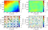 |
Fig. 4. Residuals of the comparison between PS1 and J-PLUS photometry in the r band, |
where A, B, and C are the parameters that define the plane. This provided a position-dependent zero point for each source in the pointing pid, estimated as

We present an example of this procedure for the J-PLUS pointing pid = 00315 in the lower panels of Fig. 4. The global residual, after applying the pointing-by-pointing plane correction, reduces to 0.5% (Fig. 4, upper right panel). The improvement in the photometric precision of the J-PLUS calibration thanks to the plane correction is demonstrated in Sect. 5.1, where the common sources from adjacent pointings are used to estimate the uncertainties in the calibration process.
At the end of this step, the calibration of the J-PLUS gri passbands is anchored to the PS1 photometric solution. We also calibrated the z band, and it is used as a control check of the calibration procedure in Sect. 5.3.
4.3. Step 3: homogenization with the instrumental stellar locus
In the previous section, we calibrated the J-PLUS gri broad bands via the PS1 photometry. However, we have no access to a high-quality photometric reference in the seven J-PLUS medium bands. To perform the calibration of these passbands, and of the u and z broad bands, we used the stellar and the white dwarf loci (Sect. 4.4).
The stellar locus technique assumes that the intrinsic distribution of stars defines a narrow region in colour space, and that this locus is independent of the position on the sky. Thus, we can calibrate a set of filters by matching the observed locus to a reference one (e.g. High et al. 2009; Kelly et al. 2014; Kuijken et al. 2019). First, we tested the photometric calibration of the gri bands performed in the previous section by estimating the MS stellar locus in the (𝒳 − r)0 versus (g − i)0 colour–colour diagram, where 𝒳 = {g, i}. We present these diagrams in Fig. 5. We found a clearly defined stellar locus that is parametrized with a linear interpolation from the median of the (𝒳 − r)0 colour distribution computed at (g − i)0 bins with 0.1 mag size in the range −0.5 < (g − i)0 < 2.4. The dispersion of MS stars with respect to the parametrized stellar locus is 13 mmag for the g band and 12 mmag for the i band. This exercise demonstrates that the anchoring to the PS1 photometry provides a well-calibrated gri J-PLUS magnitude, and thus can be used to study the stellar locus in the other J-PLUS passbands.
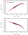 |
Fig. 5. Dust de-reddened colour–colour diagrams of the J-PLUS passbands anchored to the PS1 photometric solution. Dots are individual MS calibration stars. Upper panel: (g − r)0 vs. (g − i)0 stellar locus. Lower panel: (i − r)0 vs. (g − i)0 stellar locus. The red line in both panels shows the median stellar locus in the range −0.5 < (g − i)0 < 2.4. |
For each of the J-PLUS filters 𝒳 that we aim to calibrate, we have to construct the colour–colour diagram (𝒳 − r)0 versus (g − i)0 and define the stellar locus. Because the gri filters were already calibrated and the impact of the MW interstellar extinction had been removed, any pointing-by-pointing discrepancy with respect to the stellar locus can be attributed to the effect of the atmosphere in 𝒳 at the moment of the observation. For a given (g − i)0 colour, the stellar locus defines an intrinsic (𝒳 − r)0 colour that satisfies the following equation in each J-PLUS pointing pid,
![$$ \begin{aligned} (\mathcal{X} - r)_0^\mathrm{SL}&=\ \left\langle \ [ \mathcal{X} _{\mathrm{ins},j} - 25 + \mathrm{ZP}_{\mathcal{X} }\,(p_{\rm id},X_j,Y_j) - k_{\mathcal{X} } E(B{-}V)_j ] \right. \nonumber \\&\quad - \left.[ r_j - k_{r} E(B{-}V)_j ]\ \right\rangle , \end{aligned} $$](/articles/aa/full_html/2019/11/aa36405-19/aa36405-19-eq21.gif)
where the operator ⟨ ⋅ ⟩ denotes the median, and the locus was computed with the j sources in the pointing pid at a given (g − i)0 colour.
In the case of the J-PLUS medium bands, we have no access to the intrinsic stellar locus  . We circumvent this issue by including an extra term in the zero point,

where Δ𝒳WD is a new offset that provides the absolute calibration of the passband outside the atmosphere. In this section, we detail the estimation of Δ𝒳atm and P𝒳, and we deal with Δ𝒳WD in Sect. 4.4. We note that the calibration of gri against PS1 implies ΔgriWD ∼ 0.
We use the filter J0660 as an example in the following, but the procedure was the same in the other J-PLUS filters. We defined the initial version of the instrumental stellar locus (ISL), noted  , with a linear fit to the dust-corrected colour–colour data of those MS calibration stars in J-PLUS with 0.20 < (g − i)0 < 1.25. In this process, the magnitudes outside the atmosphere in the gri bands and the instrumental magnitudes in the J0660 band were used (upper panel in Fig. 6). Formally,
![$$ \begin{aligned} (\mathcal{X} - r)_0^\mathrm{ISL} = \left\langle \ [ \mathcal{X} _{\mathrm{ins},j} - k_{\mathcal{X} } E(B{-}V)_j ] - [ r_j - k_{r} E(B{-}V)_j ]\ \right\rangle , \end{aligned} $$](/articles/aa/full_html/2019/11/aa36405-19/aa36405-19-eq25.gif)
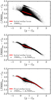 |
Fig. 6. Dust de-reddened (J0660ins − r)0 vs. (g − i)0 colour–colour diagram. Dots are individual MS calibration stars. Upper panel: initial instrumental J0660 photometry. The solid line shows the linear fit to the data in the range 0.20 < (g − i)0 < 1.25. Middle panel: J0660 photometry corrected with the offsets ΔJ0660atm. The red line shows the linear fit in the upper panel. Bottom panel: final instrumental stellar locus (red line) estimated as the median of the colour distribution in the range −0.5 < (g − i)0 < 2.4. The final ΔJ0660atm were estimated with respect to this locus. |
where the index j runs over all J-PLUS MS calibration stars at a given (g − i)0 colour. We estimated the offsets ΔJ0660atm as the median difference between the MS calibration stars with 0.20 < (g − i)0 < 1.25 in a given pointing and the initial ISL. Thanks to these initial offsets, the pointing-by-pointing differences are largely suppressed (middle panel in Fig. 6). Then, we estimated the final ISL in the range −0.5 < (g − i)0 < 2.4 with a linear interpolation from the median of the (J0660ins − r)0 + ΔJ0660atm colour distribution computed at (g − i)0 bins with 0.1 mag size. The final offset in each pointing was estimated as the difference with respect to this final locus (bottom panel in Fig. 6). We checked that extra iterations do not improve the results. After this process, the dispersion of all MS calibration stars with respect to the J0660 instrumental stellar locus had decreased from 57 mmag to 12 mmag.
The next step is to estimate the plane correction outlined in Sect. 4.2. Because we did not have access to external photometry, we used the colour distance to the final ISL as reference to define the residual:

The stacked residuals along the CCD position with respect to the final ISL are presented in the upper left panel of Fig. 7. As in the r-band case, a clear gradient emerges, but with a different direction. Because the stellar locus has its own physical dispersion, we enhanced the signal in each individual pointing by splitting the CCD into 16 regions (4 × 4 grid) and computing the median  in each of these regions (Fig. 7, lower panels). In this process, we assumed that any measured trend is due to variations in the J0660 photometry alone. Then, we fitted a plane to these median differences to obtain PJ0660 (pid, X, Y). The stacked residuals after applying the plane correction are at the 0.5% level (upper right panel in Fig. 7). The inclusion of the plane correction further decreases the dispersion with respect to the ISL to 9 mmag. As in the broad band case, the improvement in the photometry due to the plane correction is evaluated in Sect. 5.1.
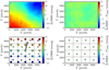 |
Fig. 7. Residuals of the comparison between the final ISL and the (J0660ins − r)0 + ΔJ0660atm colour as a function of the (X, Y) position of the source on the CCD. Upper left panel: stacked residual map of all the J-PLUS DR1 pointings. Upper right panel: stacked residual map after applying the plane correction estimated pointing-by-pointing. Lower left panel: residual map of the pointing pid = 00315. The median residuals with respect to the instrumental stellar locus in 16 regions (4 × 4 grid, dotted lines) covering the CCD (coloured circles) are fitted with a plane (coloured squares). The direction of maximum variation is shown with the arrow. Lower right panel: median differences after applying the plane correction. |
We replicated the process above with the other J-PLUS filters, obtaining a consistent photometry in all the 511 DR1 pointings. However, the reference stellar locus used for the homogenization is the median of the J-PLUS observations, and it therefore refers to the median airmass and atmospheric transparency of the survey. In other words, we have a homogeneous instrumental photometry affected by a median (unknown) atmosphere. This is convenient to reach our calibration goal, as we demonstrate in Sect. 4.4.
4.4. Step 4: absolute colour calibration with the white dwarf locus
The properties of white dwarfs make them excellent standard sources for calibration (Holberg & Bergeron 2006). The model atmospheres of WDs can be specified at the ∼1% flux level with an effective temperature (Teff) and a surface gravity (log g). These parameters can be accurately estimated by spectroscopic analysis of the Balmer line profiles, providing a reference flux model for calibration. They are also mostly photometrically stable and statistically present lower levels of interstellar reddening than main sequence stars (WDs are intrinsically faint, so we only detect the nearby ones). Because of these properties, a significant observational and theoretical effort is still underway to provide the best possible WD network to ensure a high-quality calibration of deep photometric surveys (e.g. Bohlin 2000; Holberg & Bergeron 2006; Narayan et al. 2016, 2019, and references therein).
A set of well-characterized WDs can be used to obtain global offsets in the calibration of photometric systems (Holberg & Bergeron 2006). This procedure implies two steps: first, we have to obtain the properties of the calibration WDs (effective temperature and gravity) to derive their theoretical fluxes. Second, the observed fluxes are compared to those obtained from the convolution of the WD modelled spectra with the targeted photometric system. The difference between the two measurements provides offsets that correct the initial calibration of the studied passbands.
The application of the scheme above to multi-filter surveys is severely time consuming, implying repeated observations of the sparse population of reference WDs. As an example, only one WD in the calibration network from Narayan et al. (2019) has been observed in J-PLUS DR1. Instead of the one-to-one comparison, we statistically analysed the distribution of WDs in 11 J-PLUS colour–colour diagrams (Figs. 8–10) to obtain the offsets Δ𝒳WD. These offsets translate the ISL outside the atmosphere, see Eq. (18), and complete the calibration process.
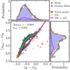 |
Fig. 8. Dust de-reddened (uins − r)0 vs. (g − i)0 colour–colour diagram of the 293 high-quality white dwarfs in J-PLUS DR1 (clean sample, cyan dots; outliers, red dots). The solid lines show the theoretical locus for DA (orange) and DB+DC WDs (magenta). The grey scale shows the most probable model that describes the observations. The blue probability distributions above and to the right show the (g − i)0 and (uins − r)0 projections of the data, respectively. The projections of the total, DA, and DB+DC models are represented with the black, orange, and magenta lines. The model in all the J-PLUS colour–colour diagrams shares the parameters μ = −0.808, s = 0.400, α = 2.65, fDA = 0.85, log g = 8.01, and Δ𝒞1 = 0.007 (see text for details). The values of the filter-dependent parameters σint and Δ𝒳WD are labelled in the panel. |
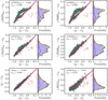 |
Fig. 9. Similar to Fig. 8, but for 𝒳 = J0378, J0395, J0410, J0430, g, and J0515 passbands. We omit the (g − i)0 projection because it is shared by all the panels. |
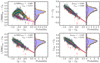 |
Fig. 10. Similar to Fig. 8, but for 𝒳 = J0660, i, J0861, and z passbands. We omit the (g − i)0 projection because it is shared by all the panels. |
The observational WD locus is well described by the theory and presents two branches, corresponding to hydrogen (DA) and helium (DB + DC) white dwarfs (e.g. Holberg & Bergeron 2006; Ivezić et al. 2007; Ibata et al. 2017; Gentile Fusillo et al. 2019; Bergeron et al. 2019). These populations are evident for 𝒳 = {u, J0378, J0395, J0660}, where the hydrogen lines are more prominent. We aim to match the WD locus estimated with J-PLUS instrumental magnitudes to the values expected from theory, obtaining the absolute colour calibration of the J-PLUS passbands. We used the r band as reference in this analysis, and thus ΔrWD = 0 by construction.
We note that the statistical analysis of the WD locus is only possible thanks to the homogenization performed in Sect. 4.3. The number density of high-quality WDs in J-PLUS DR1 is ∼0.3 deg−2 (i.e. less than one per pointing), and thus the WD locus cannot be constructed pointing-by-pointing. However, we now have a homogeneous instrumental photometry, so we can use the whole WD population present in the J-PLUS DR1 area to transport the final ISL outside the atmosphere.
The statistical modelling of the WD locus is described in Sect. 4.4.1. The WDs selected using the Gaia absolute magnitude–colour diagram (Sect. 4.1 and Fig. 2) were first cleaned from outliers (Sect. 4.4.2). Then, a joint analysis of the 11 possible (𝒳 − r)0 versus (g − i)0 colour–colour diagrams was performed to obtain the Δ𝒳WD values (Sect. 4.4.3). We present the results of this analysis in Sect. 4.4.4. The uncertainties related with the absolute colour calibration performed in this section are discussed in Sect. 5.3.
4.4.1. Modelling the WD colour–colour diagrams
We have developed several tools to use PRObability Functions for Unbiased Statistical Estimations (PROFUSE11) of galaxy distributions across cosmic time. They include galaxy luminosity functions (López-Sanjuan et al. 2017; Viironen et al. 2018), galaxy merger fractions (López-Sanjuan et al. 2015), mass-to-light ratio versus colour relations (López-Sanjuan et al. 2019a), Hα emission-line fluxes (Vilella-Rojo et al. 2015; Logroño-García et al. 2019), stellar populations (Díaz-García et al. 2015), and star/galaxy classification (López-Sanjuan et al. 2019b). In this case, we applied our previous knowledge to perform a Bayesian modelling of the white dwarf locus.
The intrinsic distribution of interest is denoted D, and provides the real values of our measurements for a set of parameters θ,
where  and
and  are the real values of the colours unaffected by both observational errors and systematic offsets. In our case,
  and
and  . We derived the posterior of the parameters θ that define the intrinsic distribution D with a Bayesian model. Formally,

where σ𝒞1 and σ𝒞2 are respectively the uncertainties in the observed (g − i)0 and (𝒳 − r)0 colours, ℒ is the likelihood of the data given θ, and P(θ) the prior in the parameters. The posterior probability is normalized to one.
The likelihood function associated with our problem is

where the index j spans the WDs in the sample, and Pj traces the probability of the measurement j for a set of parameters θ. This probability can be expressed as
where the real values  and
and  derived from the model D are affected by Gaussian observational errors,
![$$ \begin{aligned} P_G\,(x\,|\,x_0, \sigma _x) = \frac{1}{\sqrt{2 \pi } \sigma } \exp \bigg [-\frac{(x - x_0)^2}{2\sigma ^2}\bigg ], \end{aligned} $$](/articles/aa/full_html/2019/11/aa36405-19/aa36405-19-eq38.gif)
providing the likelihood of an observed colour given its real value and uncertainty. We have no access to the real values of the colours, so we marginalized over them in Eq. (24), and the likelihood is therefore expressed with known quantities.
We explored the parameters posterior distribution with the emcee code (Foreman-Mackey et al. 2013), a Python implementation of the affine-invariant ensemble sampler for the Markov chain Monte Carlo (MCMC) technique proposed by Goodman & Weare (2010). The emcee code provides a collection of solutions in the parameter space, denoted θMC, with the density of solutions being proportional to the posterior probability of the parameters. We obtained the central values of the parameters and their uncertainties from a Gaussian fit to the θMC distribution.
We define in the following the intrinsic distribution assumed for the WD locus, and the prior imposed to their parameters. The WD population was described as

where D1 provides the intrinsic (g − i)0 colour distribution, D2 describes the (𝒳 − r)0 distribution that depends on (g − i)0, and θWD = {θ1, θ2}. The (g − i)0 distribution of the WD population is not symmetric (Fig. 8), and we accounted for this asymmetry with a skew Gaussian function (Azzalini 2005),
![$$ \begin{aligned} D_{1}\,(\mathcal{C} _{1}^\mathrm{real}\,|\,\theta _1) = P_G\,(\mathcal{C} _{1}^\mathrm{real}\,|\,\mu , s)\,\bigg [1 + \mathrm{erf}\,\bigg (\alpha \,\frac{\mathcal{C} _{1}^\mathrm{real} - \mu }{\sqrt{2}s}\bigg )\bigg ], \end{aligned} $$](/articles/aa/full_html/2019/11/aa36405-19/aa36405-19-eq40.gif)
where θ1 = {μ, s, α}. The distribution in (𝒳 − r)0 is
![$$ \begin{aligned} D_{2}\,(\mathcal{C} _{2}^\mathrm{real}\,|\,\mathcal{C} _{1}^\mathrm{real}, \theta _2)&=\ \big [f_{\rm DA} P_G\,({\mathcal{C} }_{2}^\mathrm{real}\,|\,M_{\rm DA}, \sigma _{\rm int})\ \nonumber \\&\quad + (1 - f_{\rm DA}) P_G\,({\mathcal{C} }_{2}^\mathrm{real}\,|\,M_{\rm DB}, \sigma _{\rm int}) \big ], \end{aligned} $$](/articles/aa/full_html/2019/11/aa36405-19/aa36405-19-eq41.gif)
where  and
and  define the theoretical WD locus for hydrogen and helium white dwarfs with gravity log g, respectively; fDA is the fraction of DA white dwarfs in the sample; σint is the intrinsic dispersion (i.e. related to physical properties) of the WD locus; and θ2 = {fDA, log g, σint} are the parameters of the distribution.
The theoretical loci for DA and DB+DC WDs were obtained from the 3D model atmospheres presented in Tremblay et al. (2013) and Cukanovaite et al. (2018), respectively. The high-resolution spectral models at different gravities (log g = 7, 7.5, 8, 8.5, and 9) were convolved with the J-PLUS filter system to obtain the theoretical WD locus. We performed a linear interpolation in the provided colours to access other gravity values during the modelling. The colour variations due to the variety of gravities in the WD population under study are absorbed by the σint parameter.
We included at this stage two systematic offsets in the modelling, Δ𝒞1 and Δ𝒞2. These offsets affect the theoretical WD locus, displacing it to match the observed distribution. The gri broad bands are anchored to the PS1 photometric solution, implying that Δ𝒞1 ∼ 0 and Δ𝒞2 = −Δ𝒳WD. We assumed the r band as absolute reference for the J-PLUS colours, so the offset in 𝒞2 is needed to transform 𝒳 instrumental magnitudes into calibrated magnitudes outside the atmosphere.
We ended with a set of eight parameters to describe the observed colour–colour distribution of the J-PLUS WDs: θWD = {μ, s, α, fDA, log g, σint, Δ𝒞1, Δ𝒞2}. We used flat priors, P(θWD) = 1, except for the dispersions s and σint, which we imposed to be positive; the fraction of DA white dwarfs, which we imposed in the range fDA ∈ [0, 1]; and the median gravity of the WD population, which was restricted to the range log g ∈ [7, 9]. This scheme was the basis for the study of the WD population, including the removal of outlier WDs (Sect. 4.4.2) and the joint estimation of the Δ𝒳WD offsets needed to complete the photometric calibration of the J-PLUS passbands (Sect. 4.4.3).
4.4.2. Removal of outlier WDs
One of the main advantages of WDs as calibration sources is their well-known physics. However, our initial WD sample derived from Gaia data in Sect. 4.1 can be contaminated, for example by unresolved WD+M binaries, foreground galaxies and neighbouring stars in the 6″ aperture, calcium and magnetic white dwarfs that are not reproduced by our assumed theoretical tracks, and variable ZZ Ceti stars. All these kinds of sources could have colours far from the model expectations, biasing our analysis. Thus, our first goal is to clean up the initial WD sample from these physical outliers.
One way to define the clean WD sample is to visually inspect the stamps, the J-PLUS photo-spectra, and the ancillary data of the 293 initial sources to select and remove the outliers. This process is subjective and time-consuming, so we decided to apply a statistical and automatic procedure to define the outlier WDs. We included a new component in the distribution of the J-PLUS WDs to account for the presence of outlier sources. This component was defined as a uniform density and is regulated with a new parameter called fout. Formally,
where the function 𝒰 provides a uniform probability density in colour–colour space. To minimize the degeneracies between parameters in those colour–colour diagrams where DA and DB+DC white dwarfs are not well separated, we fixed μ = −0.8, s = 0.4, α = 2.8, fDA = 0.85, log g = 8, and Δ𝒞1 = 0. Thus, we only had three free parameters in this analysis, θWD = {σint, Δ𝒞2} and fout. We obtained the most probable values for these parameters and computed the probability of each white dwarf to be part of the desired WD locus. We only retained those sources with a probability higher than 97.5%, and the rest of the WDs were marked as outliers.
The selection of the outlier WDs was done in sequence, starting in the z filter and moving to the bluer passbands. We started in the reddest band because WD+M binaries, which dominate the outlier WDs, are easily detected in this colour–colour diagram. Those WDs marked as outliers in one band were not used in the subsequent analysis. With this procedure we found 28 outlier WDs, or 10% of the initial sample. We repeated the full process, starting again with the z band, and no additional WD was marked as an outlier. The remaining 265 WDs were used in the joint study presented in the next section.
4.4.3. Joint modelling of the WD locus
After removing the outlier WDs, we had a clean sample of 265 WDs. The final stage in our calibration process is to perform a joint analysis of the 11 independent colour–colour diagrams to define the offsets Δ𝒳WD. We maximized the joint probability of the 11 diagrams by multiplying their individual likelihoods from Eq. (23). We had a total of 27 free parameters in the analysis: the three parameters of the shared (g − i)0 distribution, the fraction of DA white dwarfs, the median gravity of the WD population, one intrinsic dispersion per filter (11 parameters), and one offset per filter (11 parameters, the targeted Δ𝒳WD). In the fitting process, the offset in the (g − i)0 colour was estimated as Δ𝒞1 = −Δ𝒳g + Δ𝒳i.
4.4.4. Absolute colour calibration from WD locus modelling
In this section we present the final results of the WD locus modelling and the estimation of the offsets Δ𝒳WD needed to transport the J-PLUS instrumental magnitudes to calibrated magnitudes outside the atmosphere. The analysed data and the final modelling of the WD locus are presented in Figs. 8–10. We summarize the obtained Δ𝒳WD and σint in Table 3.
Estimated offsets to transport the instrumental stellar locus outside the atmosphere, intrinsic dispersion of the WD locus, and the final median zero points in J-PLUS DR1.
We find a good agreement between the J-PLUS photometric data and the WD locus model. The (g − i)0 distribution is parametrized with μ = − 0.808 ± 0.007, s = 0.400 ± 0.007, and α = 2.65 ± 0.13. This distribution has a clear tail towards the red colours (Fig. 8), which is properly described thanks to the skewness parameter α.
We obtain a DA fraction of fDA = 0.85 ± 0.01 and a median gravity of the WD population of log g = 8.01 ± 0.03. This gravity value is similar to that obtained via previous analyses (see Jiménez-Esteban et al. 2018; Gentile Fusillo et al. 2019; Tremblay et al. 2019; Bergeron et al. 2019, and references therein). We were able to constrain these two parameters using instrumental magnitudes in most of the J-PLUS filters thanks to the presence of the DA and DB+DC branches, and to the variation of the locus curvature with the gravity.
The offsets Δ𝒳WD permit us to obtain the final zero points of the 511 J-PLUS DR1 pointings. The typical error in these offsets is ∼5 mmag, and thus a few hundred WDs are enough to provide robust results. We report the median J-PLUS zero points in Table 3. We found that the offset in the (g − i)0 colour is not zero, with ΔC1 = 7 ± 2 mmag. Thanks to the joint WD locus modelling, we were able to find residual differences in the calibration of the J-PLUS g and i passbands with respect to the PS1 photometric system (Sect. 4.2). We discuss this further in Sect. 5.3.
Finally, we comment on the values obtained for the intrinsic dispersion of the WD locus. We find that the bluer bands have a dispersion of ∼0.03 mag, larger than the ∼0.015 mag exhibited by the other filters. This highlights the greater impact of gravity variations in the photometry of the bluer J-PLUS filters and their importance for the study of individual WD properties. This analysis is beyond the scope of the present paper, and will be addressed in future works of the J-PLUS collaboration.
5. Calibration performance and error budget
The methodology presented in the previous section provides the photometric calibration of the multi-filter J-PLUS observations. In this section, we test the performance of the calibration process by studying the photometric differences of sources observed by two adjacent pointings (Sects. 5.1 and 5.2). We also discuss the absolute colour (Sect. 5.3) and flux (Sect. 5.4) uncertainties in our calibration. The impact of the assumed MW extinction is explored in Sect. 5.5. We compare the new J-PLUS calibration with the previous calibrations in Sect. 5.6. Finally, the calibrated stellar locus is compared against stellar libraries in Sect. 5.7. We summarize the error budget of the calibration process in Table 4.
Error budget of the J-PLUS photometric calibration.
5.1. Internal precision from overlapping areas
We measured the relative uncertainty (i.e. the precision) in the calibration by comparing the photometry of those MS stars observed independently in the overlapping areas between adjacent pointings. We computed the differences in the calibrated magnitudes and estimated the median of the sources shared by every pair of overlapping pointings. We obtained 1173 unique pair pointings in J-PLUS DR1. The distribution of these median differences was then used to estimate the relative uncertainty in the calibration. The distributions are nicely described by Gaussian functions and the desired precision is obtained as  , where σ is the measured dispersion. We used the pointing-by-pointing median instead of the total distribution for individual sources because (i) the calibration was performed in each pointing individually, so this is the natural reference unit; (ii) we minimized the greater statistical weight of the densest pointings; and (iii) we minimized the broadening of the distribution due to the uncertainties in the magnitude measurements.
We summarize our finding in Table 4 and Fig. 11. The relative uncertainty is ∼18 mmag in u, J0378, and J0395; ∼9 mmag in J0410 and J0430; and ∼5 mmag in the other filters. In Table 4 and Fig. 11 we also present the relative uncertainties derived with the stellar locus regression method and with our methodology when the plane correction is neglected. We found that the SLR calibration is clearly improved by the new procedure even without the plane correction at filters bluer than J0515. This is due to the inclusion of the MW extinction in our methodology, which is more prominent in the bluer bands. A great improvement in the redder bands (factor of 2–3) is feasible as a consequence of the plane correction, where this improvement is mild (∼30%) in the three bluer bands. This is due to the intrinsic properties of the stellar locus in these passbands, which is broader because of metallicity differences in the stars.
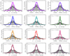 |
Fig. 11. Probability distribution of the median differences in the photometry of MS stars independently observed by two adjacent pointings. In all the panels the black histogram shows the results from the SLR (reference photometry in J-PLUS DR1), the grey filled histogram shows the results after applying Δ𝒳atm, and the coloured histogram after applying Δ𝒳atm and P𝒳 (X, Y). The solid line is the best Gaussian fit to the latest case. The uncertainty in the calibration is labelled in the panels and was estimated as the dispersion of the fitted Gaussian divided by the square root of two. Shown (from top to bottom and left to right) are the filters u, J0378, J0395, J0410, J0430, g, J0515, r, J0660, i, J0861, and z. |
The calibration methodology described in this paper assumes that the J-PLUS photometric and instrumental system does not vary with time. However, there are variations in the system due to wavelength-dependent changes in the atmospheric ozone content, airmass, humidity, mirrors reflectivity, among others. The precision reached in the calibration demonstrates that these variations are not important and the assumption of a constant photometric system is therefore valid.
We conclude that the photometric precision of J-PLUS DR1 has been improved by a factor of two with respect to previous calibration processes without the need of time consuming calibration observations or constant atmospheric monitoring.
5.2. Photometric precision from giant branch stars
We computed again the relative uncertainties as in the previous section, but now comparing the photometry of GB stars in the overlapping areas. Because GB stars are ten times less common than MS stars, the number of independent pointing pairs reduces to 409. In addition, this also increases the uncertainty in the measured median differences, enhancing the dispersion of the distribution even if the precision of the calibration remains the same.
With the above caveats in mind, the results summarized in Table 5 present the same trends and lead to the same conclusions as in Sect. 5.1. The typical dispersion in the u and J0378 bands is ∼40% larger than in the MS case. This reflects the inherent difficulties in the calibration of these passbands and their larger photometric errors. The final dispersion in the rest of the passbands is slightly larger (∼10%) with respect to the MS case in Sect. 5.1. We conclude that the zero points obtained with the MS stars also provide a good calibration for the photometry of the independent GB population. Thus, a proper calibration of any other astrophysical source in the images is expected, as is also demonstrated with the WD locus analysis presented in Sect. 4.4.
Precision of the J-PLUS photometric calibration from giant branch stars.
5.3. Colour uncertainties
The uncertainties in the colour calibration of the J-PLUS DR1 photometry are presented in Table 4. The modelling process in Sect. 4.4 provides the best solutions for Δ𝒳WD and also their dispersions, typically ∼5 mmag. These errors must be added to the uncertainties in Sect. 5.1 to have the error in the calibration when 𝒳 − r colours are analysed.
We further study the offsets implied by the WD modelling in the common PS1 filters giz. The r reference filter is discussed in the next section. We found ΔgWD = −3 ± 2 mmag and ΔiWD = 4 ± 2 mmag. In the case of the z band, we compared the final calibration zero point at each pointing estimated from the instrumental stellar and white dwarf loci (Sects 4.3 and 4.4), and by direct comparison with PS1 photometry (Sect. 4.2). We found a difference of 0 ± 5 mmag between the two procedures.
The offsets required to reach the J-PLUS photometric system from PS1 calibration are at the 5 mmag level and are always compatible at 2σ. These differences are not surprising because we used transformation equations as proxies for the differences between PS1 and J-PLUS photometric systems (Sect. 4.2). We found that the initial transformations derived from the synthetic photometry of the Pickles stellar library had ∼10 mmag colour residuals. We corrected the colour dependence of these residuals, but global offsets at this level cannot be discarded. Thanks to the white dwarf locus, we were able to estimate these global offsets.
5.4. Absolute flux uncertainty
The last source of error in our analysis is related with the absolute flux calibration determined by the reference r band. We note that any change in the r-band calibration will modify accordingly the offsets Δ𝒳WD to keep the white dwarf locus anchored. The colour offsets derived in giz from the PS1 initial calibration are at the 5 mmag level (Sect. 5.3), and we can assume a similar precision for the r band. Moreover, Narayan et al. (2019) found a 4 mmag offset between the PS1 photometry and their network of 19 WDs defined for calibration purposes. Thus, we assume a σr = 5 mmag uncertainty in the absolute flux calibration of the reference r band. We present our total error budget for absolute flux photometry in the last column of Table 4 and in Fig. 12. When compared with the SLR uncertainty given in the first column of Table 4, a factor of two improvement is reached.
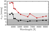 |
Fig. 12. Final calibration uncertainty in J-PLUS DR1. The black pentagons show the accuracy achieved with the calibration procedure presented in this work. The red dots show the accuracy of the SLR methodology used as reference in J-PLUS DR1. The dark (light) grey area marks a precision of 10 mmag (20 mmag). |
5.5. Impact of the assumed Milky Way extinction
One of the main assumptions in our calibration process is the extinction law used to de-redden the J-PLUS magnitudes. Because we used the 3D dust maps from Green et al. (2018), we assumed the S16 extinction law. To test the impact of this assumption in our analysis, we repeated the calibration using the Fitzpatrick (1999) extinction law and their associated coefficients, presented in Whitten et al. (2019). We find that the differences in the zero points from both extinction laws are ≲5 mmag. Thus, we conclude that the assumed extinction law has a limited impact in our calibration process.
In the estimation of the reddening, we also assumed a total-to-selective extinction ratio of RV = 3.1. This parameter varies with the position on the sky, producing different extinction curves. The J-PLUS DR1 covers one thousand square degrees, so variations in RV cannot be discarded. We can assume that the RV distribution in the area observed by J-PLUS DR1 is described by a median value ⟨RV⟩ and a dispersion σRV. Previous works find σRV ∼ 0.25 (e.g. Fitzpatrick & Massa 2007; Schlafly et al. 2016; Lee et al. 2018). This variation in RV translates into an extra dispersion in the de-reddened colours, and it is therefore included in the uncertainties listed in Table 4. It is also possible that ⟨RV⟩≠3.1, producing a systematic offset in the calibration. Studies in the literature find differences of Δ⟨RV⟩ ∼ ± 0.2 (e.g. Schultz & Wiemer 1975; Cardelli et al. 1989; Fitzpatrick & Massa 2007; Schlafly et al. 2010, 2016; Lee et al. 2018). This translates into systematic zero point differences of ≲5 mmag. As in the case of the extinction law, a limited impact is expected due to the variations of RV across the surveyed area.
5.6. Comparison with previous J-PLUS photometric calibrations
In this section we compare the previous calibration methodologies applied to J-PLUS photometry (Sect. 3) with the new proposed method. We defined the parameter

where the index m covers the different calibration methods. We did not take into account the plane correction in this exercise. We computed ΔZP𝒳, m for all the J-PLUS DR1 pointings, and present the median and the dispersion of the obtained distribution for each passband in Fig. 13. We note that some of the calibrations were performed without applying the aperture correction to the instrumental magnitudes, causing a systematic offset in the measured zero points. We accounted for the aperture correction when needed. We find the following:
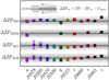 |
Fig. 13. Comparison between the different zero point estimations for J-PLUS DR1 and those presented in this work. The y-axis present the difference ΔZPm = Δ𝒳atm + Δ𝒳WD + 25 − ZPm, where the index m covers the different calibration methods: spectro-photometric standard stars (SSS), broad-band SDSS photometry (SDSS), synthetic photometry from SDSS spectra (spec), and stellar locus regression (SLR). Aperture corrections were applied to the SDSS, spec, and SLR methods (see text for details). The grey areas show differences of 0.01, 0.05, and 0.1 magnitudes in the zero points, and the dotted lines indicate identity. The points and their error bars represent the median and the dispersion of the difference distributions. |
Spectro-photometric standard stars (SSS method). The median absolute difference between the new methodology and the values obtained with SSSs is ∼0.02 mag, with all the filters but z consistent below 0.05 mag. The instrumental flux of the SSSs in the calibration images was estimated using the Moffat (1969) model, so Caper ∼ 0. The dispersion in the distribution of differences is the smallest of all the methods, suggesting that the new procedure properly traces the different atmosphere conditions. As discussed in Sect. 3, the SSS calibration is only available on photometrically stable nights. Moreover, only three sets of calibration images were acquired during an observing night to maximize scientific operation, and in several cases the SSSs were saturated in the broad-band images. All these constraints reduce the number of J-PLUS DR1 pointings fully calibrated with SSSs to 38 (7% of the total). Thus, the usual SSS calibration is not practical for J-PLUS.
Photometric comparison with SDSS broad bands (SDSS method). We find consistent zero points with differences below 0.05 mag and dispersions of ∼0.015 mag. Interestingly, there is a trend from the u band to the z band, with ΔZPugriz, SDSS = −0.045, −0.001, −0.010, 0.022, 0.029 mag; and dispersions of 0.023, 0.016, 0.013, 0.009, and 0.013 mag, respectively. These differences are consistent with the offsets estimated by Eisenstein et al. (2006) to pass from the SDSS photometric system to the AB system, ugrizAB − ugrizSDSS = −0.040, 0, 0, 0.015, 0.030 (see also Holberg & Bergeron 2006). Accounting for these expected offsets in the photometric SDSS zero points, the agreement with the new J-PLUS calibration improves to the 1% level in all cases. This is not surprising since these authors use WDs to estimate the SDSS offsets to the AB system. The final 1% agreement achieved between SDSS and J-PLUS reinforces our proposed calibration procedure.
Synthetic photometry from SDSS spectra (spec method). As in the photometric case, the zero points are consistent at 0.05 mag level, with a median absolute difference of ∼0.02 mag. There is an apparent “U” shape in the differences, with a minimum in the g band, and the dispersion in the bluer passbands is larger (≳0.05 mag). The most plausible origin of these trends is the intrinsic difficulties of a proper flux calibration of the observed spectra. Our results suggest that the global calibration of SDSS spectra in the optical is reliable at the ∼3% level.
Stellar Locus Regression (SLR method). The differences between the SLR method and our new methodology present the same trends as the initial zero points used by the SLR procedure, i.e. SDSS photometry in u and z, and SDSS spectroscopy in the rest of the passbands. As before, the systematic differences are always below 0.05 mag, with a median absolute difference of ∼0.03 mag.
The results above demonstrate that the different calibration methods applied to J-PLUS DR1 data are consistent at ∼0.03 mag level. They also suggest that our proposed calibration procedure provides J-PLUS magnitudes close to the AB system, as desired.
5.7. Comparison with stellar libraries
As a final test of the calibration process, we compared the calibrated, dust de-reddened colour–colour diagrams in J-PLUS with those expected from the empirical stellar library of Pickles (1998). We present a selection of three diagrams in Fig. 14, both for MS and GB stars. We find an overall good agreement between the empirical library and the locus of the J-PLUS sources.
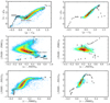 |
Fig. 14. Dust de-reddened J-PLUS colour–colour diagrams of MS (left panels) and GB stars (right panels). From top to bottom: (u − g)0 vs. (g − r)0; (J0430 − J0861)0 vs. (u − J0378)0; (J0395 − J0515)0 vs. (r − J0660)0. The colour scale shows the density of sources, increasing from blue to red. The J-PLUS colours from the synthetic photometry of the Pickles (1998) empirical library are shown as grey symbols (squares for luminosity class V and triangles for luminosity class III). The location of low-metallicity halo stars and blue horizontal branch (BHB) stars is marked with a black line in the upper and middle left panels. |
Several remarkable features are present in the chosen colour–colour diagrams. We present the usual SDSS diagram (u − g)0 versus (g − r)0 in the upper panels of Fig. 14. Two branches in (u − g)0 appear at 0.3 ≤ (g − r)0 ≤ 0.6. As shown by Ivezić et al. (2008), they are related with the disk and halo components of the MW and reflect metallicity differences in their stellar populations. The Pickles library follows the upper sequence of MW disk stars, so it is not the optimal library for studying the stellar halo of the MW. There is also a subtle MS population above the Pickles models at −0.3 ≤ (g − r)0 ≤ 0, populated by blue horizontal branch (BHB) stars. For the GB population, we find a lack of spectral types bluer than F5 and redder than M5. This is related with the area surveyed by J-PLUS, which avoids the MW disk, and the high-quality photometric selection, which penalizes red stars with low flux in the bluer passbands.
The features in the previous diagram are enhanced with the J-PLUS medium bands in the middle panels of Fig. 14. The (J0430 − J0861)0 versus (u − J0378)0 diagram clearly shows the BHB population, split from the main sequence locus at (u − J0378)0 > 0.65. In addition, the lower metallicity halo population is better traced, with the second branch noticeable at (u − J0378)0 > 0.3 and (J0430 − J0861)0 > 0.5.
Finally, we present the (J0395 − J0515)0 versus (r − J0660)0 diagram in the lower panels of Fig. 14. In this case, we highlight the J-PLUS capabilities to trace different stellar gravities. For colours redder than (r − J0660)0 ∼ 0.1, MS stars exhibit a nearly constant colour (J0395 − J0515)0 ∼ 2.2. In contrast, the population of red giants does not approach a constant regime, reaching (J0395 − J0515)0 ∼ 3.2.
We have shown the capabilities of the J-PLUS photometric system to trace different properties and populations of MW stars, and have demonstrated the agreement of the final calibrated J-PLUS photometry with the popular empirical library of Pickles (1998). We conclude that J-PLUS offers a well-calibrated photometry to conduct both MW (e.g. Bonatto et al. 2019; Whitten et al. 2019) and extragalactic studies (e.g. Molino et al. 2019; Logroño-García et al. 2019; San Roman et al. 2019).
6. Application of the new calibration to J-PLUS data
The calibration methodology presented in Sect. 4 has been applied to J-PLUS DR1 data. We provide four parameters per pointing and filter: Z, A, B, and C. The first parameter encapsulates the atmospheric and white dwarf offsets:

We provide Z in the ADQL table jplus.CalibTileImage. The parameters A, B, and C, which define the position dependence of the zero point, are reported in the ADQL table jplus.TileImage.
The new zero point for each source is estimated as

where SWDL refers to the “stellar and white dwarf loci” calibration method presented in this paper, and (X, Y) is the position of the sources in the CCD12.
We simplified the updating process by pre-computing the needed magnitude and flux transformations. They are included in the J-PLUS database as column zpt_swdl_calc. Extra information and ADQL examples to directly retrieve the updated photometry from the database can be found in the J-PLUS webpage13.
Regarding the uncertainty in the photometry, the catalogues available at the J-PLUS database provide photon and sky background errors. Thus, the calibration error must be added by the user as
where σ𝒳 is the error in the magnitude from the database and σcal is the calibration error in Table 4. We note that this action is also needed for any other J-PLUS calibration.
Finally, we also provide the new ADQL table jplus. CalibStarsSWDL, which lists the type (MS, GB, WD, outlier WD) and the E(B − V) colour excess of the high-quality calibration stars used in the present paper.
6.1. Application to future J-PLUS data
The SWDL calibration will be set as the default calibration procedure in subsequent J-PLUS data releases.
Its application to those images taken after DR1 does not require repeating the full process. The definition of the high-quality stars in the pointing using Gaia information (Sect. 4.1) and the calibration of the gri broad bands with PS1 photometry, including the plane correction (Sect. 4.2), are needed. Then, the instrumental stellar locus step (Sect. 4.3) can be simplified. The final ISL computed with J-PLUS DR1 have been recorded, and the new observations can be compared to these previously computed loci to estimate the observational offsets Δ𝒳atm. The plane correction is then estimated. Finally, the offsets Δ𝒳WD reported in Table 3 should be applied. This process is illustrated in Fig. 15. We note that the WD offsets are attached to the definition of the ISL, so only a re-computation of the ISL will request a new estimation of Δ𝒳WD. This simplified version of the methodology will speed up the calibration process.
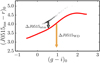 |
Fig. 15. Illustration of the simplified calibration process for J-PLUS images beyond DR1. The J0515 passband and the DR1 pointing pid = 03508 are used as example. The offset Δ𝒳atm (grey arrow) is estimated with respect to the ISL computed with DR1 data (red solid line). The global offset Δ𝒳WD given in Table 3 is then applied to obtain the final zero point (coloured arrow). |
The precision of the photometric calibration in future J-PLUS data could be degraded if the new observations target highly extinct areas in comparison with the DR1. However, we find that the integrated colour excess distribution at the central coordinates of the total 4 599 J-PLUS pointings is similar to the distribution of the 511 DR1 pointings (Fig. 16). Thus, the precision achieved in J-PLUS DR1 should be representative of the whole J-PLUS project and similar figures are expected at survey completion.
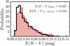 |
Fig. 16. Probability distribution of the integrated colour excess E(B − V) estimated at the centre of the J-PLUS pointings. We show the distribution for J-PLUS DR1 (511 pointings, red hatched histogram) and for the full J-PLUS area (4599 pointings, black histogram). The median colour excess of each case is labelled in the panel. |
6.2. Application to other surveys
In addition to J-PLUS, the proposed calibration method can be applied to other surveys. For example, the images acquired with J-PLUS passbands beyond the J-PLUS project can be also calibrated. In this case, the final ISL and the WD analysis must be repeated using PS1 photometry directly in the gri broad bands. We recall that both Gaia and PS1 cover all of the observable sky from OAJ. Thanks to the computed ISL and Δ𝒳WD, the proper calibration of any single T80Cam image will be possible without the need of extra calibration images.
We plan to apply this calibration method to J-PAS, which will observe several thousand square degrees with 56 narrow optical filters. Irrespective of the changes imposed by the J-PAS observing strategy, the main steps developed in the present paper will be accordingly adapted and tested. Given the deeper J-PAS observations and the expected abundance of WDs, the ∼1% accuracy in most of the J-PAS passbands would be reached after gathering ∼500 deg2 of data. We recall that the J-PAS footprint is identical to the J-PLUS one, so the discussion of the impact of the extinction in Sect. 6.1 also applies to J-PAS.
Finally, we also briefly comment on the Gaia DR3, which will contain low-resolution spectrophotometry in the optical. Gaia DR3 will provide an independent reference to calibrate both J-PLUS and J-PAS. More importantly, the WD locus absolute colour calibration presented in Sect. 4.4 should be a competitive method to calibrate the Gaia spectrophotometric data. We will explore this possibility in the future.
7. Summary and conclusions
We presented an optimized method for performing the photometric calibration of the large-area multi-filter J-PLUS project. The method has four main steps:
-
Definition of a high-quality set of calibration stars using Gaia information and the available 3D dust maps from Green et al. (2018).
-
Anchoring of the J-PLUS gri passbands to the PS1 photometric solution. We accounted for the variation of the calibration with source position on the CCD, that presents a gradient component.
-
Homogenization of the photometry in the other nine J-PLUS filters using the dust de-reddened instrumental stellar locus in (𝒳 − r)0 versus (g − i)0 colours. In this case, the zero point variation along the CCD is estimated from the distance to the stellar locus.
-
Absolute colour calibration with the white dwarf locus. We performed a joint Bayesian modelling of 11 observed J-PLUS colour–colour diagrams, including DA and DB+DC branches and removing outlier WDs, by using the theoretical white dwarf locus from Tremblay et al. (2013) and Cukanovaite et al. (2018). This provides the offsets needed to transform instrumental magnitudes to calibrated AB magnitudes outside the atmosphere.
The final uncertainty of the J-PLUS photometric calibration, estimated from duplicated objects observed in adjacent pointings and accounting for the absolute colour and flux calibration errors, are ∼19 mmag in u, J0378 and J0395, ∼11 mmag in J0410 and J0430, and ∼8 mmag in g, J0515, r, J0660, i, J0861, and z. These accuracies were achieved with neither long observing campaigns for calibration nor constant atmospheric monitoring. We compared the calibrated colour–colour J-PLUS diagrams with those expected from the empirical stellar library of Pickles (1998), and find a good agreement.
We provide the instructions and the parameters needed to update the J-PLUS DR1 photometry to the new calibration frame (Sect. 6). The proposed method will be set as the default calibration procedure in subsequent J-PLUS data releases. We plan to adapt the methodology for the photometric calibration of J-PAS, which will observe several thousand square degrees with 56 narrow optical filters. Given the deeper J-PAS observations and the expected abundance of WDs, the ∼1% accuracy in most of the J-PAS passbands would be reached after gathering ∼500 deg2 of data. This will permit a great number of high-quality cosmological, extragalactic, and Milky Way related studies during the next decades.
Acknowledgments
We dedicate this paper to the memory of our six IAC colleagues and friends who met with a fatal accident in Piedra de los Cochinos, Tenerife, in February 2007, with special thanks to Maurizio Panniello, whose teachings of python were so important for this paper. We thank the anonymous referee for useful comments and suggestions. Based on observations made with the JAST/T80 telescope at the Observatorio Astrofísico de Javalambre (OAJ), in Teruel, owned, managed, and operated by the Centro de Estudios de Física del Cosmos de Aragón. We acknowledge the OAJ Data Processing and Archiving Unit (UPAD) for reducing and calibrating the OAJ data used in this work. Funding for the J-PLUS Project has been provided by the Governments of Spain and Aragón through the Fondo de Inversiones de Teruel; the Aragón Government through the Reseach Groups E96, E103, and E16_17R; the Spanish Ministry of Science, Innovation and Universities (MCIU/AEI/FEDER, UE) with grants PGC2018-097585-B-C21 and PGC2018-097585-B-C22; the Spanish Ministry of Economy and Competitiveness (MINECO) under AYA2015-66211-C2-1-P, AYA2015-66211-C2-2, AYA2012-30789, and ICTS-2009-14; and European FEDER funding (FCDD10-4E-867, FCDD13-4E-2685). This work was also supported by the MINECO through grant ESP2016-80079-C2-1-R and RTI2018-095076-B-C21 (MINECO/FEDER, UE) and MDM-2014-0369 of ICCUB (Unidad de Excelencia “María de Maeztu”). F. J. E. acknowledges financial support from the Tec2Space-CM project (P2018/NMT-4291). Funding for the SDSS and SDSS-II has been provided by the Alfred P. Sloan Foundation, the Participating Institutions, the National Science Foundation, the U.S. Department of Energy, the National Aeronautics and Space Administration, the Japanese Monbukagakusho, the Max Planck Society, and the Higher Education Funding Council for England. The SDSS Web Site is www.sdss.org. The SDSS is managed by the Astrophysical Research Consortium for the Participating Institutions. The Participating Institutions are the American Museum of Natural History, Astrophysical Institute Potsdam, University of Basel, University of Cambridge, Case Western Reserve University, University of Chicago, Drexel University, Fermilab, the Institute for Advanced Study, the Japan Participation Group, Johns Hopkins University, the Joint Institute for Nuclear Astrophysics, the Kavli Institute for Particle Astrophysics and Cosmology, the Korean Scientist Group, the Chinese Academy of Sciences (LAMOST), Los Alamos National Laboratory, the Max-Planck-Institute for Astronomy (MPIA), the Max-Planck-Institute for Astrophysics (MPA), New Mexico State University, the Ohio State University, University of Pittsburgh, University of Portsmouth, Princeton University, the United States Naval Observatory, and the University of Washington. The Pan-STARRS1 Surveys (PS1) and the PS1 public science archive have been made possible through contributions by the Institute for Astronomy, the University of Hawaii, the Pan-STARRS Project Office, the Max-Planck Society and its participating institutes, the Max Planck Institute for Astronomy, Heidelberg, and the Max Planck Institute for Extraterrestrial Physics, Garching, The Johns Hopkins University, Durham University, the University of Edinburgh, the Queen’s University Belfast, the Harvard-Smithsonian Center for Astrophysics, the Las Cumbres Observatory Global Telescope Network Incorporated, the National Central University of Taiwan, the Space Telescope Science Institute, the National Aeronautics and Space Administration under Grant No. NNX08AR22G issued through the Planetary Science Division of the NASA Science Mission Directorate, the National Science Foundation Grant No. AST-1238877, the University of Maryland, Eotvos Lorand University (ELTE), the Los Alamos National Laboratory, and the Gordon and Betty Moore Foundation. This work has made use of data from the European Space Agency (ESA) mission Gaia (https://www.cosmos.esa.int/gaia), processed by the Gaia Data Processing and Analysis Consortium (DPAC, https://www.cosmos.esa.int/web/gaia/dpac/consortium). Funding for the DPAC has been provided by national institutions, in particular the institutions participating in the Gaia Multilateral Agreement. This research made use of Astropy, a community-developed core Python package for Astronomy (Astropy Collaboration 2013), and Matplotlib, a 2D graphics package used for Python for publication-quality image generation across user interfaces and operating systems (Hunter 2007).
References
- Abazajian, K. N., Adelman-McCarthy, J. K., Agüeros, M. A., et al. 2009, ApJS, 182, 543 [NASA ADS] [CrossRef] [Google Scholar]
- Aihara, H., AlSayyad, Y., Ando, M., et al. 2019, PASJ, in press [arXiv:1905.12221] [Google Scholar]
- Astropy Collaboration (Robitaille, T. P., et al.) 2013, A&A, 558, A33 [NASA ADS] [CrossRef] [EDP Sciences] [Google Scholar]
- Azzalini, A. 2005, Scand. J. Stat., 32, 159 [CrossRef] [Google Scholar]
- Bailer-Jones, C. A. L., Rybizki, J., Fouesneau, M., Mantelet, G., & Andrae, R. 2018, AJ, 156, 58 [NASA ADS] [CrossRef] [Google Scholar]
- Benítez, N., Dupke, R., Moles, M., et al. 2014, ArXiv e-prints [arXiv:1403.5237] [Google Scholar]
- Bergeron, P., Dufour, P., Fontaine, G., et al. 2019, ApJ, 876, 67 [NASA ADS] [CrossRef] [Google Scholar]
- Bertin, E., & Arnouts, S. 1996, A&AS, 117, 393 [NASA ADS] [CrossRef] [EDP Sciences] [Google Scholar]
- Bohlin, R. C. 2000, AJ, 120, 437 [NASA ADS] [CrossRef] [Google Scholar]
- Bonatto, C., Chies-Santos, A. L., Coelho, P. R. T., et al. 2019, A&A, 622, A179 [NASA ADS] [CrossRef] [EDP Sciences] [Google Scholar]
- Burke, D. L., Saha, A., Claver, J., et al. 2014, AJ, 147, 19 [NASA ADS] [CrossRef] [Google Scholar]
- Burke, D. L., Rykoff, E. S., Allam, S., et al. 2018, AJ, 155, 41 [NASA ADS] [CrossRef] [Google Scholar]
- Cardelli, J. A., Clayton, G. C., & Mathis, J. S. 1989, ApJ, 345, 245 [NASA ADS] [CrossRef] [Google Scholar]
- Cenarro, A. J., Moles, M., Marín-Franch, A., et al. 2014, in Observatory Operations: Strategies, Processes, and Systems V, Proc. SPIE, 9149, 91491I [Google Scholar]
- Cenarro, A. J., Moles, M., Cristóbal-Hornillos, D., et al. 2019, A&A, 622, A176 [NASA ADS] [CrossRef] [EDP Sciences] [Google Scholar]
- Chambers, K. C., Magnier, E. A., Metcalfe, N., et al. 2016, ArXiv e-prints [arXiv:1612.05560] [Google Scholar]
- Covey, K. R., Ivezić, Ž., Schlegel, D., et al. 2007, AJ, 134, 2398 [NASA ADS] [CrossRef] [Google Scholar]
- Cukanovaite, E., Tremblay, P. E., Freytag, B., Ludwig, H. G., & Bergeron, P. 2018, MNRAS, 481, 1522 [Google Scholar]
- Danielski, C., Babusiaux, C., Ruiz-Dern, L., Sartoretti, P., & Arenou, F. 2018, A&A, 614, A19 [NASA ADS] [CrossRef] [EDP Sciences] [Google Scholar]
- Dey, A., Schlegel, D. J., Lang, D., et al. 2019, AJ, 157, 168 [NASA ADS] [CrossRef] [Google Scholar]
- Díaz-García, L. A., Cenarro, A. J., López-Sanjuan, C., et al. 2015, A&A, 582, A14 [NASA ADS] [CrossRef] [EDP Sciences] [Google Scholar]
- Dye, S., Lawrence, A., Read, M. A., et al. 2018, MNRAS, 473, 5113 [NASA ADS] [CrossRef] [Google Scholar]
- Eisenstein, D. J., Liebert, J., Harris, H. C., et al. 2006, ApJS, 167, 40 [NASA ADS] [CrossRef] [Google Scholar]
- Epchtein, N., Deul, E., Derriere, S., et al. 1999, A&A, 349, 236 [NASA ADS] [Google Scholar]
- Finkbeiner, D. P., Schlafly, E. F., Schlegel, D. J., et al. 2016, ApJ, 822, 66 [NASA ADS] [CrossRef] [Google Scholar]
- Fitzpatrick, E. L. 1999, PASP, 111, 63 [NASA ADS] [CrossRef] [Google Scholar]
- Fitzpatrick, E. L., & Massa, D. 2007, ApJ, 663, 320 [NASA ADS] [CrossRef] [EDP Sciences] [Google Scholar]
- Flaugher, B. 2012, in APS April Meeting Abstracts, D7007 [Google Scholar]
- Flewelling, H. A., Magnier, E. A., Chambers, K. C., et al. 2016, ArXiv e-prints [arXiv:1612.05243] [Google Scholar]
- Foreman-Mackey, D., Hogg, D. W., Lang, D., & Goodman, J. 2013, PASP, 125, 306 [CrossRef] [Google Scholar]
- Gaia Collaboration, (Prusti, T., et al.) 2016, A&A, 595, A1 [NASA ADS] [CrossRef] [EDP Sciences] [Google Scholar]
- Gaia Collaboration (Brown, A. G. A., et al.) 2018a, A&A, 616, A1 [NASA ADS] [CrossRef] [EDP Sciences] [Google Scholar]
- Gaia Collaboration (Babusiaux, C., et al.) 2018b, A&A, 616, A10 [NASA ADS] [CrossRef] [EDP Sciences] [Google Scholar]
- Gal, R. R., de Carvalho, R. R., Odewahn, S. C., et al. 2004, AJ, 128, 3082 [NASA ADS] [CrossRef] [Google Scholar]
- Gentile Fusillo, N. P., Tremblay, P.-E., Gänsicke, B. T., et al. 2019, MNRAS, 482, 4570 [NASA ADS] [CrossRef] [Google Scholar]
- Goodman, J., & Weare, J. 2010, Comm. App. Math. Comp. Sci., 5, 65 [Google Scholar]
- Green, G. M., Schlafly, E. F., Finkbeiner, D., et al. 2018, MNRAS, 478, 651 [NASA ADS] [CrossRef] [Google Scholar]
- High, F. W., Stubbs, C. W., Rest, A., Stalder, B., & Challis, P. 2009, AJ, 138, 110 [NASA ADS] [CrossRef] [Google Scholar]
- Holberg, J. B., & Bergeron, P. 2006, AJ, 132, 1221 [NASA ADS] [CrossRef] [EDP Sciences] [Google Scholar]
- Hunter, J. D. 2007, Comput. Sci. Eng., 9, 90 [NASA ADS] [CrossRef] [Google Scholar]
- Ibata, R. A., Lewis, G. F., McConnachie, A. W., et al. 2014, ApJ, 780, 128 [NASA ADS] [CrossRef] [Google Scholar]
- Ibata, R. A., McConnachie, A., Cuillandre, J. C., et al. 2017, ApJ, 848, 128 [NASA ADS] [CrossRef] [Google Scholar]
- Ivezić, Ž., Smith, J. A., Miknaitis, G., et al. 2007, AJ, 134, 973 [NASA ADS] [CrossRef] [Google Scholar]
- Ivezić, Ž., Sesar, B., Jurić, M., et al. 2008, ApJ, 684, 287 [NASA ADS] [CrossRef] [Google Scholar]
- Ivezic, Z., Kahn, S. M., Tyson, J. A., et al. 2019, ApJ, 873, 111 [NASA ADS] [CrossRef] [Google Scholar]
- Jiménez-Esteban, F. M., Torres, S., Rebassa-Mansergas, A., et al. 2018, MNRAS, 480, 4505 [NASA ADS] [CrossRef] [Google Scholar]
- Kelly, P. L., von der Linden, A., Applegate, D. E., et al. 2014, MNRAS, 439, 28 [NASA ADS] [CrossRef] [Google Scholar]
- Kuijken, K., Heymans, C., Dvornik, A., et al. 2019, A&A, 625, A2 [NASA ADS] [CrossRef] [EDP Sciences] [Google Scholar]
- Laureijs, R., Amiaux, J., Arduini, S., et al. 2011, ArXiv e-prints [arXiv:1110.3193] [Google Scholar]
- Le Borgne, J. F., Bruzual, G., Pelló, R., et al. 2003, A&A, 402, 433 [NASA ADS] [CrossRef] [EDP Sciences] [Google Scholar]
- Lee, A., Green, G. M., Schlafly, E. F., et al. 2018, ApJ, 854, 79 [NASA ADS] [CrossRef] [Google Scholar]
- Logroño-García, R., Vilella-Rojo, G., López-Sanjuan, C., et al. 2019, A&A, 622, A180 [NASA ADS] [CrossRef] [EDP Sciences] [Google Scholar]
- López-Sanjuan, C., Cenarro, A. J., Varela, J., et al. 2015, A&A, 576, A53 [NASA ADS] [CrossRef] [EDP Sciences] [Google Scholar]
- López-Sanjuan, C., Tempel, E., Benítez, N., et al. 2017, A&A, 599, A62 [NASA ADS] [CrossRef] [EDP Sciences] [Google Scholar]
- López-Sanjuan, C., Díaz-García, L. A., Cenarro, A. J., et al. 2019a, A&A, 622, A51 [NASA ADS] [CrossRef] [EDP Sciences] [Google Scholar]
- López-Sanjuan, C., Vázquez Ramió, H., Varela, J., et al. 2019b, A&A, 622, A177 [NASA ADS] [CrossRef] [EDP Sciences] [Google Scholar]
- Lorenzo-Gutiérrez, A., Alfaro, E. J., Maíz Apellániz, J., et al. 2019, MNRAS, 486, 966 [NASA ADS] [CrossRef] [Google Scholar]
- Luri, X., Brown, A. G. A., Sarro, L. M., et al. 2018, A&A, 616, A9 [NASA ADS] [CrossRef] [EDP Sciences] [Google Scholar]
- Magnier, E. A., Chambers, K. C., Flewelling, H. A., et al. 2016a, ArXiv e-prints [arXiv:1612.05240] [Google Scholar]
- Magnier, E. A., Schlafly, E. F., Finkbeiner, D. P., et al. 2016b, ArXiv e-prints [arXiv:1612.05242] [Google Scholar]
- Magnier, E. A., Sweeney, W. E., Chambers, K. C., et al. 2016c, ArXiv e-prints [arXiv:1612.05244] [Google Scholar]
- Maíz Apellániz, J., & Weiler, M. 2018, A&A, 619, A180 [NASA ADS] [CrossRef] [EDP Sciences] [Google Scholar]
- Marín-Franch, A., Taylor, K., Cenarro, J., Cristobal-Hornillos, D., & Moles, M. 2015, IAU General Assembly, 29, 2257381 [Google Scholar]
- McMahon, R. G., Banerji, M., Gonzalez, E., et al. 2013, The Messenger, 154, 35 [NASA ADS] [Google Scholar]
- Mendes de Oliveira, C., Ribeiro, T., Schoenell, W., et al. 2019, MNRAS, 489, 241 [NASA ADS] [CrossRef] [Google Scholar]
- Moffat, A. F. J. 1969, A&A, 3, 455 [NASA ADS] [Google Scholar]
- Molino, A., Costa-Duarte, M. V., de Mens Oliveira, C., et al. 2019, A&A, 622, A178 [NASA ADS] [CrossRef] [EDP Sciences] [Google Scholar]
- Narayan, G., Axelrod, T., Holberg, J. B., et al. 2016, ApJ, 822, 67 [NASA ADS] [CrossRef] [Google Scholar]
- Narayan, G., Matheson, T., Saha, A., et al. 2019, ApJS, 241, 20 [NASA ADS] [CrossRef] [Google Scholar]
- Ofek, E. O., Laher, R., Law, N., et al. 2012, PASP, 124, 62 [NASA ADS] [CrossRef] [Google Scholar]
- Oke, J. B., & Gunn, J. E. 1983, ApJ, 266, 713 [NASA ADS] [CrossRef] [Google Scholar]
- Padmanabhan, N., Schlegel, D. J., Finkbeiner, D. P., et al. 2008, ApJ, 674, 1217 [NASA ADS] [CrossRef] [MathSciNet] [Google Scholar]
- Pickles, A. J. 1998, PASP, 110, 863 [CrossRef] [Google Scholar]
- Regnault, N., Conley, A., Guy, J., et al. 2009, A&A, 506, 999 [NASA ADS] [CrossRef] [EDP Sciences] [Google Scholar]
- San Roman, I., Sánchez-Blázquez, P., Cenarro, A. J., et al. 2019, A&A, 622, A181 [NASA ADS] [CrossRef] [EDP Sciences] [Google Scholar]
- Schlafly, E. F., Finkbeiner, D. P., Schlegel, D. J., et al. 2010, ApJ, 725, 1175 [NASA ADS] [CrossRef] [Google Scholar]
- Schlafly, E. F., Finkbeiner, D. P., Jurić, M., et al. 2012, ApJ, 756, 158 [NASA ADS] [CrossRef] [Google Scholar]
- Schlafly, E. F., Meisner, A. M., Stutz, A. M., et al. 2016, ApJ, 821, 78 [NASA ADS] [CrossRef] [Google Scholar]
- Schultz, G. V., & Wiemer, W. 1975, A&A, 43, 133 [NASA ADS] [Google Scholar]
- Scolnic, D., Casertano, S., Riess, A., et al. 2015, ApJ, 815, 117 [NASA ADS] [CrossRef] [Google Scholar]
- Skrutskie, M. F., Cutri, R. M., Stiening, R., et al. 2006, AJ, 131, 1163 [NASA ADS] [CrossRef] [Google Scholar]
- Smee, S. A., Gunn, J. E., Uomoto, A., et al. 2013, AJ, 146, 32 [Google Scholar]
- Starkenburg, E., Martin, N., Youakim, K., et al. 2017, MNRAS, 471, 2587 [NASA ADS] [CrossRef] [Google Scholar]
- Tonry, J. L., Stubbs, C. W., Lykke, K. R., et al. 2012, ApJ, 750, 99 [NASA ADS] [CrossRef] [Google Scholar]
- Tremblay, P. E., Cukanovaite, E., Gentile Fusillo, N. P., Cunningham, T., & Hollands, M. A. 2019, MNRAS, 482, 5222 [NASA ADS] [CrossRef] [EDP Sciences] [Google Scholar]
- Tremblay, P. E., Ludwig, H. G., Steffen, M., & Freytag, B. 2013, A&A, 559, A104 [NASA ADS] [CrossRef] [EDP Sciences] [Google Scholar]
- Varela, J., & Cristóbal-Hornillos, D. 2017, https://doi.org/10.5281/zenodo.1039008 [Google Scholar]
- Viironen, K., López-Sanjuan, C., Hernández-Monteagudo, C., et al. 2018, A&A, 614, A129 [NASA ADS] [CrossRef] [EDP Sciences] [Google Scholar]
- Vilella-Rojo, G., Viironen, K., López-Sanjuan, C., et al. 2015, A&A, 580, A47 [NASA ADS] [CrossRef] [EDP Sciences] [Google Scholar]
- Waters, C. Z., Magnier, E. A., Price, P. A., et al. 2016, ArXiv e-prints [arXiv:1612.05245] [Google Scholar]
- Wittman, D., Ryan, R., & Thorman, P. 2012, MNRAS, 421, 2251 [NASA ADS] [CrossRef] [Google Scholar]
- Whitten, D. D., Placco, V. M., Beers, T. C., et al. 2019, A&A, 622, A182 [NASA ADS] [CrossRef] [EDP Sciences] [Google Scholar]
- Wolf, C., Onken, C. A., Luvaul, L. C., et al. 2018, PASA, 35, e010 [Google Scholar]
- Zhou, Z., Zhou, X., Zou, H., et al. 2018, PASP, 130, 085001 [NASA ADS] [CrossRef] [Google Scholar]
All Tables
Compilation of finished (F), on-going (O), and scheduled (S) optical and near-infrared large-area (≳5000 deg2) photometric surveys.
J-PLUS photometric system, extinction coefficients, and limiting magnitudes (5σ, 3″ aperture) of J-PLUS DR1 (Cenarro et al. 2019).
Estimated offsets to transport the instrumental stellar locus outside the atmosphere, intrinsic dispersion of the WD locus, and the final median zero points in J-PLUS DR1.
All Figures
|
Fig. 1. Flowchart of the calibration method presented in this work. Arrows that originate in small dots indicate that the preceding data product is an input to the subsequent analysis. Datasets are shown with their project logo, and external codes or models with grey boxes. The rounded-shape boxes show the calibration steps. The asterisks indicate those steps based on dust de-reddened magnitudes. The white boxes show intermediate data products, and ovals highlight publicly available data products of the calibration process. |
| In the text | |
|
Fig. 2. Absolute magnitude in the G band vs. GBP − GRP colour diagram, corrected for dust reddening, of the 496 798 high-quality sources in common between J-PLUS DR1 and Gaia DR2. The black dots are individual measurements. The coloured solid contours show density of objects, starting on 25 mag−2 and increasing by a factor of ten in each step. We define three populations on this diagram: main sequence stars (465 583; white area), giant branch stars (30 922; grey area), and white dwarfs (293; blue area). |
| In the text | |
|
Fig. 3. Probability distribution of the colour excess E(B − V) for the three populations defined in the absolute magnitude vs. colour diagram: main sequence stars (MS, orange hatched histogram), giant branch stars (GB, red histogram), and white dwarfs (WD, blue filled histogram). The median colour excess of each population is labelled in the panel. |
| In the text | |
|
Fig. 4. Residuals of the comparison between PS1 and J-PLUS photometry in the r band, |
| In the text | |
|
Fig. 5. Dust de-reddened colour–colour diagrams of the J-PLUS passbands anchored to the PS1 photometric solution. Dots are individual MS calibration stars. Upper panel: (g − r)0 vs. (g − i)0 stellar locus. Lower panel: (i − r)0 vs. (g − i)0 stellar locus. The red line in both panels shows the median stellar locus in the range −0.5 < (g − i)0 < 2.4. |
| In the text | |
|
Fig. 6. Dust de-reddened (J0660ins − r)0 vs. (g − i)0 colour–colour diagram. Dots are individual MS calibration stars. Upper panel: initial instrumental J0660 photometry. The solid line shows the linear fit to the data in the range 0.20 < (g − i)0 < 1.25. Middle panel: J0660 photometry corrected with the offsets ΔJ0660atm. The red line shows the linear fit in the upper panel. Bottom panel: final instrumental stellar locus (red line) estimated as the median of the colour distribution in the range −0.5 < (g − i)0 < 2.4. The final ΔJ0660atm were estimated with respect to this locus. |
| In the text | |
|
Fig. 7. Residuals of the comparison between the final ISL and the (J0660ins − r)0 + ΔJ0660atm colour as a function of the (X, Y) position of the source on the CCD. Upper left panel: stacked residual map of all the J-PLUS DR1 pointings. Upper right panel: stacked residual map after applying the plane correction estimated pointing-by-pointing. Lower left panel: residual map of the pointing pid = 00315. The median residuals with respect to the instrumental stellar locus in 16 regions (4 × 4 grid, dotted lines) covering the CCD (coloured circles) are fitted with a plane (coloured squares). The direction of maximum variation is shown with the arrow. Lower right panel: median differences after applying the plane correction. |
| In the text | |
|
Fig. 8. Dust de-reddened (uins − r)0 vs. (g − i)0 colour–colour diagram of the 293 high-quality white dwarfs in J-PLUS DR1 (clean sample, cyan dots; outliers, red dots). The solid lines show the theoretical locus for DA (orange) and DB+DC WDs (magenta). The grey scale shows the most probable model that describes the observations. The blue probability distributions above and to the right show the (g − i)0 and (uins − r)0 projections of the data, respectively. The projections of the total, DA, and DB+DC models are represented with the black, orange, and magenta lines. The model in all the J-PLUS colour–colour diagrams shares the parameters μ = −0.808, s = 0.400, α = 2.65, fDA = 0.85, log g = 8.01, and Δ𝒞1 = 0.007 (see text for details). The values of the filter-dependent parameters σint and Δ𝒳WD are labelled in the panel. |
| In the text | |
|
Fig. 9. Similar to Fig. 8, but for 𝒳 = J0378, J0395, J0410, J0430, g, and J0515 passbands. We omit the (g − i)0 projection because it is shared by all the panels. |
| In the text | |
|
Fig. 10. Similar to Fig. 8, but for 𝒳 = J0660, i, J0861, and z passbands. We omit the (g − i)0 projection because it is shared by all the panels. |
| In the text | |
|
Fig. 11. Probability distribution of the median differences in the photometry of MS stars independently observed by two adjacent pointings. In all the panels the black histogram shows the results from the SLR (reference photometry in J-PLUS DR1), the grey filled histogram shows the results after applying Δ𝒳atm, and the coloured histogram after applying Δ𝒳atm and P𝒳 (X, Y). The solid line is the best Gaussian fit to the latest case. The uncertainty in the calibration is labelled in the panels and was estimated as the dispersion of the fitted Gaussian divided by the square root of two. Shown (from top to bottom and left to right) are the filters u, J0378, J0395, J0410, J0430, g, J0515, r, J0660, i, J0861, and z. |
| In the text | |
|
Fig. 12. Final calibration uncertainty in J-PLUS DR1. The black pentagons show the accuracy achieved with the calibration procedure presented in this work. The red dots show the accuracy of the SLR methodology used as reference in J-PLUS DR1. The dark (light) grey area marks a precision of 10 mmag (20 mmag). |
| In the text | |
|
Fig. 13. Comparison between the different zero point estimations for J-PLUS DR1 and those presented in this work. The y-axis present the difference ΔZPm = Δ𝒳atm + Δ𝒳WD + 25 − ZPm, where the index m covers the different calibration methods: spectro-photometric standard stars (SSS), broad-band SDSS photometry (SDSS), synthetic photometry from SDSS spectra (spec), and stellar locus regression (SLR). Aperture corrections were applied to the SDSS, spec, and SLR methods (see text for details). The grey areas show differences of 0.01, 0.05, and 0.1 magnitudes in the zero points, and the dotted lines indicate identity. The points and their error bars represent the median and the dispersion of the difference distributions. |
| In the text | |
|
Fig. 14. Dust de-reddened J-PLUS colour–colour diagrams of MS (left panels) and GB stars (right panels). From top to bottom: (u − g)0 vs. (g − r)0; (J0430 − J0861)0 vs. (u − J0378)0; (J0395 − J0515)0 vs. (r − J0660)0. The colour scale shows the density of sources, increasing from blue to red. The J-PLUS colours from the synthetic photometry of the Pickles (1998) empirical library are shown as grey symbols (squares for luminosity class V and triangles for luminosity class III). The location of low-metallicity halo stars and blue horizontal branch (BHB) stars is marked with a black line in the upper and middle left panels. |
| In the text | |
|
Fig. 15. Illustration of the simplified calibration process for J-PLUS images beyond DR1. The J0515 passband and the DR1 pointing pid = 03508 are used as example. The offset Δ𝒳atm (grey arrow) is estimated with respect to the ISL computed with DR1 data (red solid line). The global offset Δ𝒳WD given in Table 3 is then applied to obtain the final zero point (coloured arrow). |
| In the text | |
|
Fig. 16. Probability distribution of the integrated colour excess E(B − V) estimated at the centre of the J-PLUS pointings. We show the distribution for J-PLUS DR1 (511 pointings, red hatched histogram) and for the full J-PLUS area (4599 pointings, black histogram). The median colour excess of each case is labelled in the panel. |
| In the text | |
Current usage metrics show cumulative count of Article Views (full-text article views including HTML views, PDF and ePub downloads, according to the available data) and Abstracts Views on Vision4Press platform.
Data correspond to usage on the plateform after 2015. The current usage metrics is available 48-96 hours after online publication and is updated daily on week days.
Initial download of the metrics may take a while.