| Issue |
A&A
Volume 631, November 2019
|
|
|---|---|---|
| Article Number | A150 | |
| Number of page(s) | 12 | |
| Section | Extragalactic astronomy | |
| DOI | https://doi.org/10.1051/0004-6361/201936285 | |
| Published online | 13 November 2019 | |
The γ-ray sky seen at X-ray energies
I. Searching for the connection between X-rays and γ-rays in Fermi BL Lac objects⋆
1
Dipartimento di Fisica, Università degli Studi di Torino, Via Pietro Giuria 1, 10125 Turin, Italy
e-mail: This email address is being protected from spambots. You need JavaScript enabled to view it.
2
Facultad de Ciencias Astronómicas y Geofísicas, Universidad Nacional de La Plata, Paseo del Bosque, B1900FWA La Plata, Argentina
3
INFN – Istituto Nazionale di Fisica Nucleare, Sezione di Torino, Via Pietro Giuria 1, 10125 Turin, Italy
4
Instituto de Astrofísica de La Plata, CONICET–UNLP, CCT La Plata, Paseo del Bosque, B1900FWA La Plata, Argentina
5
INAF – Osservatorio di Astrofisica e Scienza dello Spazio, Via Gobetti 93/3, 40129 Bologna, Italy
6
Departamento de Ciencias Fisicas, Universidad Andres Bello, Fernandez Concha 700, Las Condes, Santiago, Chile
7
Center for Astrophysics | Harvard & Smithsonian, 60 Garden St, Cambridge, MA 02138, USA
8
Universidade de São Paulo, Instituto de Astronomia, Geofísica e Ciências Atmosféricas, Departamento de Astronomia, São Paulo, SP 05508-090, Brazil
Received:
10
July
2019
Accepted:
3
September
2019
Abstract
Context. BL Lac objects are an extreme type of active galactic nuclei (AGNs) that belong to the largest population of γ-ray sources: blazars. This class of AGNs shows a double-bumped spectral energy distribution that is commonly described in terms of a synchrotron self-Compton (SSC) emission process, whereas the low-energy component that dominates their emission between the infrared and the X-ray band is tightly connected to the high-energy component that peaks in the γ-rays. Two strong connections that link radio and mid-infrared emission of blazars to the emission in the γ-ray band are well established. They constitute the basis for associating γ-ray sources with their low-energy counterparts.
Aims. We searched for a possible link between X-ray and γ-ray emissions for the subclass of BL Lacs using all archival Swift/XRT observations combined with Fermi data for a selected sample of 351 sources.
Methods. Analyzing ∼2400 ks of Swift/XRT observations that were carried out until December 2018, we discovered that above the γ-ray flux threshold Fγ ≈ 3 × 10⁻¹² erg cm−2 s−1, 96% of all Fermi BL Lacs have an X-ray counterpart that is detected with signal-to-noise ratio > 3.
Results. We did not find any correlation or clear trend between X-ray and γ-ray fluxes and/or spectral shapes, but we discovered a correlation between the X-ray flux and the mid-infrared color. Finally, we discuss on a possible interpretation of our results in the SSC framework.
Key words: galaxies: active / galaxies: nuclei / galaxies: jets / BL Lacertae objects: general / X-rays: galaxies / gamma rays: galaxies
Full Table 1 is only available at the CDS via anonymous ftp to cdsarc.u-strasbg.fr (130.79.128.5) or via http://cdsarc.u-strasbg.fr/viz-bin/cat/J/A+A/631/A150
© ESO 2019
1. Introduction
Blazars are a peculiar class of active galactic nuclei (AGNs) that is characterized by emission arising from a relativistic jet oriented at small angles (e.g., less than a few degrees, Lister et al. 2013) with respect to the line of sight. This jet emission overwhelms most of the radiation of their host galaxy (Blandford & Rees 1978).
Blazar emission is detected at all frequencies. It extends from radio (see, e.g., Jorstad et al. 2001; Ciaramella et al. 2004; Ghirlanda et al. 2010; Lister et al. 2019) and even low radio frequencies (see, e.g., Nori et al. 2014; Giroletti et al. 2016, for recent observational campaigns), infrared (IR, see, e.g., Impey & Neugebauer 1988; Stevens et al. 1994; Massaro et al. 2011a; D’Abrusco et al. 2012) and optical (see, e.g., Carini et al. 1992; Marchesini et al. 2016, 2019a; Peña-Herazo et al. 2017a, for recent observational campaigns) to X-rays (see, e.g., Singh & Garmire 1985; Giommi et al. 1990; Sambruna et al. 1996; Pian et al. 1998; Paggi et al. 2013; Landi et al. 2015). The emission is also detected in the γ-ray band (see, e.g., Aharonian et al. 2005; Albert et al. 2007; Giannios et al. 2009; Tavecchio et al. 2011; Wehrle et al. 1998; Ackermann et al. 2015) and shows strong variability. It also has flaring states in which spectral shape and/or luminosities change (see, e.g., Hartman et al. 2001; Romero et al. 2002; Böttcher et al. 2007; Pandey et al. 2017; Kaur et al. 2017; Bruni et al. 2018).
Blazars can be classified into two main categories: flat-spectrum radio quasars, and BL Lac objects. Empirically, the distinction between these two classes is based on emission features in their optical spectra (Stickel et al. 1991). The first class shows strong and broad emission lines that are typical of normal quasars, while the spectra of the second class are almost featureless (i.e., emission lines with equivalent widths smaller than 5 Å). We here adopt the nomenclature established by Roma-BZC at (Massaro et al. 2015a), where flat-spectrum radio quasars are labeled BZQs and BL Lac objects are BZBs.
Blazars are the dominant class of active galaxies in the γ-ray sky (Hartman et al. 1999; Mattox & Ormes 2002; Massaro et al. 2015b). In particular, ∼56% of all associated and classified γ-ray sources that have been detected by the Fermi Large Area Telescope (Fermi-LAT) four-year Point Source Catalog (3FGL) belong to this class (Acero et al. 2015). In the past decade, follow-up spectroscopic campaigns (see, e.g., Massaro et al. 2014; Álvarez Crespo et al. 2016a,b; Peña-Herazo et al. 2017b; Marchesini et al. 2019b) confirmed that most of the sources that were classified as “Blazar Candidates of Uncertain type” (BCUs), introduced in the 3FGL catalog, are indeed blazars of BL Lac type (Massaro et al. 2016; Álvarez Crespo et al. 2016c). The same situation occurs in the preliminary version of the latest release of the Fermi catalog (Fermi-LAT Collaboration 2019; Peña-Herazo et al. 2019). Moreover, follow-up campaigns of unassociated or unidentified γ-ray sources (UGSs) have also shown that a large portion of them appear to be associated with blazars (Paggi et al. 2014; Massaro et al. 2015c; Landoni et al. 2015; Ricci et al. 2015).
The spectral energy distribution (SED) of blazars shows two components: the low-energy component peaks between infrared and X-rays, and the high-energy component peaks between hard X-rays and the γ-ray band. The low-energy component is attributed to synchrotron emission arising from electrons that are accelerated in the blazar jets, and the high-energy component is due to the inverse Compton (IC) process (see, e.g., Ghisellini et al. 1985; Maraschi et al. 1992; Massaro et al. 2006; Tramacere et al. 2007, 2011; Finke et al. 2008; Paggi et al. 2009a, for recent analyses). For BZBs in particular, the two emission processes are strictly connected because seed photons for the IC emission are emitted by electrons through synchrotron radiation (i.e., the synchrotron self-Compton, or SSC, scenario).
Two different subclasses were originally defined for BZBs to distinguish them on the basis of the ratio of their radio- to X-ray flux (Maselli et al. 2010): low-energy peaked BL Lacs (i.e., LBLs) and high-energy peaked BL Lacs (i.e., HBLs). This ratio is defined as  , where FSX is the X-ray flux from the ROSAT (short for Röntgensatellit) survey (Voges et al. 1999) in the 0.1−2 keV band, S1.4Δν is the radio flux density at 1.4 GHz multiplied by the band frequency width Δν. Thus, values of ΦXR > 1 point toward an HBL classification, while values < 1 indicate an LBL type of source. This corresponds to the limit
  .
.
A strong link between γ-ray and radio emission in blazars, known as the γ-to-radio connection (Stecker et al. 1993; Taylor et al. 2007; Bloom 2008; Ghirlanda et al. 2011), was discovered soon after the launch of the Energetic Gamma Ray Experiment Telescope (EGRET) on board the Compton Gamma-ray satellite (Fichtel et al. 1993). This link was later confirmed through Fermi observations (Mahony et al. 2010; Ackermann et al. 2011; Ghirlanda et al. 2011; Cutini et al. 2014; Lico et al. 2014).
Moreover, combining γ-ray and mid-infrared observations, the latter collected with the Wide-field Infrared Survey Explorer (WISE; Wright et al. 2010), a tight connection between their emissions in these two bands has also been discovered (Massaro et al. 2011a, 2012a; D’Abrusco et al. 2013; Massaro & D’Abrusco 2016). In particular, the γ-ray – infrared connection is strongly related not only to the blazar power, but also to their spectral shapes in the two different energy ranges; this is expected given the theoretical interpretation of their SED.
These two connections strongly stimulated follow-up campaigns to search for blazar-like counterparts of UGSs, for example, in the radio band (Massaro et al. 2013a; Nori et al. 2014; Lico et al. 2014; Giroletti et al. 2016) and/or by applying statistical procedures to find them in the WISE catalogs (D’Abrusco et al. 2013; Massaro et al. 2013a; D’Abrusco et al. 2014, 2019). On the other hand, X-ray follow-up observations have also been carried out to search for blazar-like counterparts of UGSs (e.g., Mirabal 2009; Kataoka et al. 2012; Stroh & Falcone 2013; Paggi et al. 2013; Masetti et al. 2013; Landi et al. 2015; Paiano et al. 2017), even if these counterparts not supported by any firmly established observational link or connection between the X-ray and γ-ray emission of blazars.
Based on the SSC scenario that underlies the interpretation of BL Lac SEDs, a link between X-ray and γ-ray emission could be expected because emission of the low- and high-energy components is related to the same particle distribution. This is the main aim of the analysis presented here. We focus on BZBs, whose γ-ray emission is probably not significantly contaminated by inverse Compton radiation of seed photons that arises from regions outside the jet (Sikora et al. 2013).
We aim to determine the portion of γ-ray blazars that have an X-ray counterpart with respect to their γ-ray flux, and whether their γ-ray emission (i.e., flux and/or spectral shape) correlates with the X-ray emission, as occurs in the radio and in the mid-infrared bands. Our investigation will provide the necessary scientific background to support and justify ongoing (Stroh & Falcone 2013) and future X-ray follow-up campaigns of Fermi UGSs. A detailed study of the general behavior of BZBs in the X-ray band is crucial to improve the selection of BZB candidates within a UGS sample. Our search for a connection between X-rays and γ-rays is also supported by the fact that HBLs that are detected at TeV energies (e.g., Piner & Edwards 2014, 2018) are generally among the brightest X-ray sources in the extragalactic sky and their X-ray emission is also linked to the mid-infrared emission (Massaro et al. 2013b).
To carry out our investigation, we analyzed observations from the X-ray Telescope (XRT) o board the Neil Gehrels Swift Observatory, performed before mid-December 2018, of γ-ray BZBs observed by Fermi. We made this choice because the ROSAT survey is relatively shallow. Only ∼60% percent of all known Fermi blazars are listed in the ROSAT survey catalog (Voges et al. 1999). Nevertheless, Swift performs an X-ray follow-up campaign of Fermi UGSs1 (Falcone 2013; Stroh & Falcone 2013; Falcone et al. 2014). An extensive database is therefore available.
This paper is organized as follows. In Sect. 2 we present the sample selection criteria, while in Sect. 3 we describe the Swift/XRT data reduction procedures. Section 4 is devoted to results of our analysis, and in Sect. 5 we describe a possible interpretation of our results within the SSC framework. Finally, Sect. 6 is dedicated to a brief summary and our main conclusions.
Unless stated otherwise and throughout the whole paper, we adopted cgs units and a flat cosmology with H0 = 72 km s−1 Mpc−1, and ΩΛ = 0.74 (Dunkley et al. 2009). Spectral indices α were defined so that the flux density Sν ∝ ν−α, considering α < 0.5 as flat spectra. The AllWISE magnitudes in the [3.4] μm, [4.6] μm, and [12] μm nominal filters are in the Vega system, and are not corrected for Galactic extinction because this correction is negligible for Galactic latitudes |b| > 10° (see, e.g., D’Abrusco et al. 2013).
2. Sample selection
To assess whether the X-ray and γ-ray emission in BZBs is connected, we started by selecting all known Fermi BZBs listed in the “clean” sample of the Third Catalog of Active Galactic Nuclei detected by the Fermi-LAT (Ackermann et al. 2015, 3LAC), and considered only those that belong to the fifth release of the Roma-BZCat (Massaro et al. 2015a). At this selection step our sample contained 580 of the original 1151 sources. All BZBs in BZCat have a counterpart in at least one of the main radio surveys (White et al. 1997; Condon et al. 1998; Mauch et al. 2003), and all selected BZBs are uniquely associated with γ-ray sources in the 3FGL catalog.
We only included in our sample Swift/XRT observations that were performed in photon-counting (PC) mode that lay within a circular region of 6 arcmin angular separation around the BZB γ-ray positions (431 sources). Our choice of 6 arcmin corresponds to the average semimajor axis of the positional uncertainty ellipse of γ-ray sources listed in the 3FGL (Acero et al. 2015). We chose only sources with total exposure times of between 1 and 20 ks because those with cumulative exposure times longer than 20 ks are generally pointed as follow-up observations of flaring states and are not snapshot observations. A similar criterion was adopted by Mao et al. (2016).
The Swift X-ray campaign of UGSs is performed with a nominal 5 ks exposure time (Stroh & Falcone 2013), implying that the results achieved for our selected sample are suitable to carry out a future investigation of UGSs observed with Swift/XRT (Marchesini et al., in prep.). Most of the observed fields have a 5 ks exposure time; the average of our sample is 6.7 ks.
3. Swift/XRT data reduction and analysis
3.1. Data processing
We adopted the same data reduction procedure as described in Massaro et al. (2008a,b, 2011b, 2012b), Paggi et al. (2013). Here we report the basic details and highlight differences and improvements with respect to our previous analyses.
Raw Swift/XRT data were download and reduced to obtain clean event files with the standard procedures using the XRTPIPELINE task, which is part of the Swift X-Ray Telescope Data Analysis Software (XRTDAS, Capalbi et al. 2005), and the High Energy Astrophysics Science Archive Research Center (HEASARC) calibration database (CALDB) version X20180710. In particular, using XSELECT, we excluded time intervals with count rates exceeding 40 counts per second, and time intervals where the CCD temperature exceeds −50°C in regions located at the CCD edge (D’Elia et al. 2013).
Clean event files were merged using the XSELECT task, while corresponding exposure maps were merged with XIMAGE software. Figure 1 shows a merged image obtained for the XRT field associated with 5BZB J2005+7752 as an example of the final product obtained with our code.
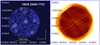 |
Fig. 1. X-ray image in the 0.5−10 keV energy range obtained by merging all XRT observations within 6 arcmin measured from the γ-ray position of 5BZB J2005+7752 (left panel) and its corresponding merged exposure map (right panel). The bright source in the center is the X-ray counterpart of the BZB, marked with the white circle as all other background and foreground X-ray sources. This X-ray image has been built by merging five observations for an exposure time of 15.9 ks. The image is also smoothed with a Gaussian kernel with a radius of 5 pixels. |
3.2. Source detection and photometry
A first detection run was performed over merged event files using the DET algorithm in XIMAGE, to obtain pixel positions for every detection with signal-to-noise ratios (S/N) > 3. Because the exposure times chosen to carry out our investigation were relatively short, we focused on a photometric analysis.
We ran the SOSTA task available within the XIMAGE package on the pixel positions obtained from DET. In particular, SOSTA takes into account the local background for each source to claim a detection, which achieves a more precise photometry than the DET algorithm. This was carried out on merged event files for the full 0.5−10 keV band, and also for the soft (0.5−2 keV) and hard (2−10 keV) bands. Sources detected with SOSTA all had an S/N between 3 and 25.
We compared the resulting X-ray sources with those listed in the Swift/XRT point source (1SXPS) catalog (Evans et al. 2014). Our procedure differs from that of 1SXPS in (i) the choice of the S/N threshold applied to claim a detection, which is S/N > 1.6, (ii) the total number of Swift/XRT observations processed (1SXPS used those up to October 2012, while we reduced those up to December 2018), and (iii) the choice of background regions (whose shape and size depend on the S/N of the source in 1SXPS). However, we found that our results agree with the 1SXPS catalog with differences of only a few percent (i.e., < 5%) mainly due to the reasons highlighted above.
Thus, we obtained positions, counts, and count rates for all sources. We flagged sources with full-band count rates > 0.5 photons per second, indicating the presence of pile-up. These are 13 sources, all of them with mild pile-up (i.e., with count rates lower than one photon per second). We then derived the hardness ratio (HRX) for each source and full-band X-ray fluxes (FX). The hardness ratio was computed as (H − S)/(H + S), where H are counts in the hard band (2−10 keV) and S those in the soft band (0.5−2 keV). We verified that using counts or count rates to obtain HRX is equivalent because the exposure map is not energy dependent in the 0.5−10 keV band. Fluxes were obtained for each source using PIMMS (Mukai 1993), assuming a power law with a photon index of 2.0 and values of the Galactic column density values obtained from the LAB Survey of Galactic HI (Kalberla et al. 2005). The choice of the photon index affects the estimate of the X-ray flux by a factor of less than a few percent (Massaro et al. 2011c, 2012c). In Table 1 we report the X-ray data and information available from cross-matches that were performed with multifrequency archives (see Sect. 4.1 for details). In Col. 1 we report the BZCat name, in Cols. 2−4 the total counts and their error for the soft (0.5−2.0 keV), hard (2.0−10 keV), and total (0.5−10 keV) bands, in Cols. 5−10 the AllWISE magnitudes and their errors, and in Col. 11 the ratio of the X-ray to radio flux.
Main results of our analysis (first 10 rows).
4. Results
4.1. X-ray counterparts of γ-ray BL Lac objects
In total, we found 1362 X-ray sources in the 351 BZB fields we reduced and analyzed. In Fig. 2 we show the distribution of the total exposure times of our final sample, of all observed fields, considering those with at least one X-ray detection and those with no X-ray sources above an S/N of 3, separately. In 14 BZBs fields no XRT counterpart was found. All these sources were observed for a total exposure time shorter than 2.4 ks, with two exceptions: 5BZB J1458+3720 (5.3 ks) and 5BZB J0434−2342 (6.8 ks). The first does not show any detection in the XRT merged observation, and the second shows two X-ray sources at more than 6 arcmin from the BZB position. There is, however, a marginal detection with an S/N of 2.8 coincident with the BZB position. This is also detected in the 1SXPS catalog with an S/N of 1.9. Both were discarded because no detection above the S/N threshold of 3 was reported. Thus the lack of X-ray counterparts for these 14 cases is mainly imputable to our choice of the S/N threshold combined with short exposure time.
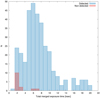 |
Fig. 2. Distribution of the total exposure time for all selected BZBs. The blue histogram indicates the X-ray merged event files with at least one X-ray source detected with an S/N > 3, while in red we show those without an X-ray detection. |
The following cuts were also performed a posteriori:
1. Spurious X-ray detections due to artifacts and bad pixels or bad columns were discarded.
2. X-ray sources that were detected close (i.e., closer than 8 arcsec) to a bright source were discarded as artifacts of the detection algorithm. The only exception was the source with the highest S/N.
3. Sources that were clearly extended with respect to the XRT 90% point spread function (PSF; 23 arcsec, Moretti et al. 2004) were discarded.
4. Sources not coincident with the BZB position (i.e., beyond 5.5 arcsec) and with negative counts on either soft and hard band (defined in Sect. 3.2) were discarded.
5. 5BZB J1104+3812 (also known as Mrk 421), which presented severe pile-up contamination, was also discarded. Mrk 421 has been thoroughly studied in γ-rays and X-rays (e.g., Brinkmann et al. 2005; Isobe et al. 2010; Banerjee et al. 2019; Hervet et al. 2019, and references therein).
6. Two BZBs that lie in the same field within the positional uncertainty region of the same Fermi source, 3FGL J0323.6−0109 (i.e., 5BZB J0323−0111 and 5BZB J0323−0108), were also discarded because of possible source confusion in γ-rays.
In addition, we also cross-matched the X-ray positions with the AllWISE catalog with an uncertainty radius of 3.3 arcsec, following D’Abrusco et al. (2013). All mid-infrared counterparts were correctly associated with the XRT detections, with two exceptions: 5BZB J0335−4459 (at 3.8 arcsec) and 5BZB J2131−2515 (at 3.5 arcsec)2. Because they are the closest WISE sources and unique matches, we kept these two BZBs in our sample.
Of the 351 Fermi BZBs observed by Swift/XRT for 1−20 ks, 337 were detected and 14 were not. In addition, 3 BZBs were discarded because of pile-up or source confusion. Thus, we built a clean sample of 334 BZBs with X-ray and mid-infrared counterparts, and a clean sample of 675 background and foreground X-ray sources lying within an angular separation of 6 arcmin from the γ-ray position. The flow chart shown in Fig. 3 summarizes all our selection steps.
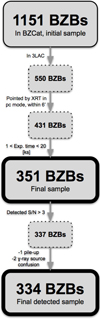 |
Fig. 3. Flow chart to highlight all steps we followed to build our final BZBs sample. |
4.2. X-ray properties of γ-ray BL Lac objects
We detected 337 BZBs using XRT data out of the original selected sample of 351 Fermi BZBs. This means that 96% of the BZB sources listed by Fermi show an X-ray counterpart when they are observed for more than 1 ks. This strongly supports the existence of a connection between X-rays and γ-rays and certainly motivates X-ray follow-up observations at least to the level of the γ-ray flux of our current BZB sample to search for UGS counterparts (Massaro et al. 2013c).
In Fig. 4 we show the distribution of the γ-ray energy flux in the 100 MeV−100 GeV band for all Fermi BZBs in our sample, divided into those for which we found at least one X-ray counterpart and those for which no XRT counterpart was detected. We plot the γ-ray flux thresholds above which we found at least one X-ray counterpart for 100% (Fγ = 1.7 × 10⁻¹¹ erg cm−2 s), 98% (Fγ = 7.0 × 10⁻¹² erg cm−2 s), and 96% (Fγ = 2.9 × 10⁻¹² erg cm−2 s) of the sample. We expect that these thresholds can be used to find new BZBs among the Fermi UGSs.
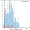 |
Fig. 4. Distribution of Fγ in the 100 MeV−100 GeV band for all 351 BZBs in our selected sample. As in Fig. 2, the blue histogram indicates the X-ray merged event file with at least one X-ray source detected with S/N > 3, and in red we show those without an X-ray detection. The solid black line corresponds to the threshold above which 100% of the selected BZBs has an X-ray counterpart, while the dashed and dot-dashed black lines mark the 98% and 96% thresholds, respectively. |
The nominal exposure time used for the UGS XRT follow-up campaign is 5 ks (Stroh & Falcone 2013). Thus, we verified the fraction of BZBs that could be detected by rescaling the exposure time to this nominal value. We selected only sources for which the total (merged) exposure time was longer than 5 ks (222 sources), and then scaled their S/N assuming a Poisson distribution of the observed count rates. We confirm that 98% of our selected sample would still be detected at an S/N > 3 with shorter (i.e., 5 ks) exposure time.
The HBL versus LBL classification was made following Maselli et al. (2010), as mentioned in Sect. 1. The 1.4 GHz radio fluxes were taken from BZCat for each source, with the exception of 5BZB J1326−5256 and 5BZB J1604−4441, for which only the flux at 4.85 GHz was available. We assumed that the spectral shape of blazars is flat (radio spectral index equal to zero) at radio frequencies (see, e.g., Healey et al. 2007; Massaro et al. 2013a,d), therefore we considered the 4.85 GHz flux to be equal to that at 1.4 GHz. Because the XRT band (0.5−10 keV) differs from that of ROSAT (0.1−2.4 keV), which is the band that was originally used for this classification, we compared the use of full-band fluxes adjusted to the ROSAT band assuming a power law. The HBL and LBL classification is the same using either of the X-ray flux estimates. Then we adopted full-band XRT fluxes. In Table 1 we show the full-band XRT-to-radio flux ratio FX/S1.4 instead of ΦXR, so that the limit between classes is FX/S1.4 > 10−11.
In total, 175 sources out of the total 334 are HBLs, while the remaining 159 are classified as LBLs. As expected, errors in HRX and FX for HBL and LBL objects are smaller than for background or foreground objects because BZBs are generally one order of magnitude brighter (average flux FX = 3.9 × 10⁻¹² erg cm−2 s−1) than background or foreground objects (average flux FX = 2.7 × 10⁻¹³ erg cm−2 s−1). On the other hand, HBLs and LBLs have softer X-ray spectra than background or foreground objects, which span all the possible HRX values. In Fig. 5 we show FX versus HRX plotted for all detected sources (i.e., BZBs and background or foreground X-ray objects). BZBs are separated into HBLs and LBLs with a color code indicating their ΦXR value, which extends from green (HBLs) to orange (LBLs), while sources with ΦXR ≈ 1 are marked in yellow. The average value for the HRX is HRX = −0.63 ± 0.09 for HBLs and HRX = −0.46 ± 0.16 for LBLs. Sources with FX > 2.0 × 10⁻¹¹ erg cm−2 s−1 (indicated with the black solid line) suffer from pile-up. The HBL and LBL subsamples lie in different regions, as do background or foreground objects. Intermediate sourcespg (i.e., with ΦXR ≈ 1) lie in between both regions, as expected. This is also true in all figures shown from this point on.
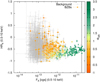 |
Fig. 5. FX in the 0.5−10 keV band vs. HRX for all BZBs in the selected sample. Background or foreground X-ray sources are marked in gray, and BZB classified as HBL and as LBL are marked in green and orange, respectively. The solid black line separates BZBs with pile-up, which show FX > 2.0 × 10⁻¹¹ erg cm−2 s−1. |
To quantify the separation between each subsample in the FX–HRX space, we performed a kernel density estimation (KDE) analysis, in order to estimate density thresholds for each subsample, following D’Abrusco et al. (2009, 2019), Laurino et al. (2011), Massaro et al. (2011a, 2013c), and references therein. In Fig. 6 we show FX versus HRX for background or foreground objects and for BZBs separated into HBLs and LBLs, with contours obtained from the KDE analysis for each subsample at 70%, 80%, and 90% isodensity levels drawn on the basis of the probability evaluated with the KDE. Although the subsamples overlap, the overlap is smallest when we consider a 90% density level. Moreover, HBLs lie in a very distinct region at all density levels.
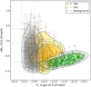 |
Fig. 6. FX in the 0.5−10 keV band vs. HRX for all BZBs in the selected sample, same as in Fig. 5. We show the 70%, 80%, and 90% isodensity contours as obtained from a KDE analysis for background or foreground sources in gray, HBLs in green, and LBLs in orange. |
From Figs. 5 and 6, it follows that the LBL and HBL classification following Maselli et al. (2010) coincides with our results obtained through a KDE analysis, with intermediate-type objects populating the overlapping isodensity area between both classes. In Fig. 7 we also show the distribution of the angular separation between the X-ray and the γ-ray positions in the same field. X-ray detected BZBs on average appear to be closer to their γ-ray counterpart than background X-ray sources in the examined fields. This is confirmed through a Kolmogorov–Smirnov test, which yields a negligible chance coincidence probability, or p-chance p. This implies a low contamination by background or foreground sources.
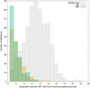 |
Fig. 7. Angular separation between the X-ray and γ-ray position for all BZBs, in arcminutes. As in Fig. 5, BZBs classified as HBLs and LBLs are shown in green and orange, respectively, while background or foreground X-ray sources are shown in gray. |
In Fig. 8 we report FX versus the WISE mid-infrared magnitude at 12 μm (in the upper panel), and versus the γ-ray energy flux in the 100 MeV−100 GeV band, taken from the 3FGL catalog (in the upper panel). The 12 μm magnitude is the least affected by Galactic extinction but is still more sensitive than the W4 magnitude at 22 μm (D’Abrusco et al. 2012). No clear trend is visible in either panel of Fig. 8. This is expected because while γ-rays are dominated by the IC SED component, X-rays are due to synchrotron emission in HBLs but might be a combination of synchrotron and IC components in LBLs (Bondi et al. 2001; Massaro et al. 2008b). No clear trend is visible between FX and the γ-ray energy flux. However, we highlight that because 96% γ-ray BZBs have a counterpart in the X-rays, this provides a direct link between the BZB emission in these two energy ranges. We recall that HBLs are on average an order of magnitude brighter in X-rays than LBLs. The average FX value is (4.5 ± 3.3)×10−12 erg cm−2 s−1 for HBLs, and (4.5 ± 1.9)×10−13 erg cm−2 s−1 for LBLs. On the other hand, LBLs are on average 0.6 mag brighter in mid-infrared than HBLs.
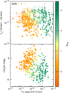 |
Fig. 8. Lower panel: FX in the 0.5−10 keV band vs. the WISE magnitude at 12 μm for all selected BZBs. Upper panel: FX in the 0.5−10 keV band vs. the Fγ in the 100 MeV−100 GeV band, collected from the 3FGL. BL Lac objects classified as HBLs and LBLs are shown in green and orange, respectively. |
The distinction between HBLs and LBLs becomes clearer when we compare their X-ray, γ-ray, and mid-infrared spectral shapes. In Fig. 9 we show FX versus the mid-infrared color computed with WISE magnitudes at 4.6 μm and 12 μm (upper panel) and versus the γ-ray spectral index reported in the 3FGL (lower panel). HBLs are brighter in X-rays and harder in γ-rays than LBLs (Ghisellini et al. 2010, 2017). In the lower panel of Fig. 9 we also plot the average and median values of these parameters for both samples, together with their standard deviation and median absolute deviation, to highlight the clear distinction between the two subclasses. Although we were unable to establish a clear trend between fluxes or spectral shapes of BZBs in the X-ray and γ-ray band, we proved that there is a link between the emission in these two energy ranges given by the Fermi BZB high detection rate in the Swift/XRT observations analyzed here.
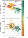 |
Fig. 9. Upper panel: FX in the 0.5−10 keV band vs. the [4.6]−[12] μm mid-infrared color. Selected BZBs are classified as HBLs and LBLs and are marked in green and orange, respectively. Dashed lines indicate regression lines for LBLs (purple), HBLs (red), and the whole sample (black). Lower panel: FX in the 0.5−10 keV band vs. the αγ as reported in the 3FGL. Solid black lines mark the area within one standard deviation centered on the mean, and solid gray shows the area computed with the median absolute deviation centered on the median value. |
This is different from what was discovered between radio, mid-infrared, and γ-ray emission for this class of AGNs, but it is crucial to support ongoing and future X-ray campaigns searching for blazars within sample of UGSs as well as for spectroscopic follow-up observations of X-ray sources that lie within the positional uncertainty region of unassociated Fermi sources.
The previous distinction improves significantly when the mid-infrared color is used, mainly because it marks the difference in the synchrotron component between HBLs and LBLs better. We found a correlation between FX and the [4.6]−[12] μm WISE color index, with a slope of ∼ − 0.32 and a p-chance of p < 1 × 10⁻⁷ for the whole sample of BZBs (plotted as the black line in Fig. 9). This is due to the shifting of the whole synchrotron component toward higher energies because X-rays and infrared trace two different sides of the synchrotron peak. The trend is clearer for HBLs than for LBLs possibly because the IC component in the SEDs of the latter subclass might contribute. The p-chance of both correlations is p ∼ 3.7 × 10⁻⁷ for HBLs (plotted in red) and p ∼ 0.019 for LBLs (plotted in purple), indicating that the second is not statistically significant. In almost all previous WISE and X-ray combined investigations (see, e.g., Maselli et al. 2013), the lack of uniform X-ray datasets did not allow a comparison of the behavior of HBLs and LBLs, as done here.
In Fig. 10 we show HRX versus the mid-infrared color and versus the γ-ray spectral index. We note that HBLs tend to cover a small range of X-ray hardness ratios; they appear to have softer X-ray spectra than LBLs. The average value for the HRX is −0.63 ± 0.09 for HBLs and −0.46 ± 0.16 for LBLs. The opposite occurs for the γ-ray spectral index and mid-infrared colors, where HBLs show a wider range of values than LBLs.
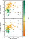 |
Fig. 10. Comparison of the spectral shape for all the BZBs in our sample. LBLs are shown in orange and HBLs in green. Upper panel: HRX in the 0.5−10 keV band vs. the [4.6]−[12] μm mid-infrared color. Lower panel: HRX in the 0.5−10 keV band vs. αγ. In both panels the average uncertainties on the parameters are shown as crosses in the top right corner. |
Finally, for 77 BZBs a redshift estimate was available in Roma-BZCat, allowing us to compute their X-ray luminosities (LX), as shown in Fig. 11. HBLs tend to be more luminous than LBLs in the X-ray band. This might be due to the redshift difference, which on average is 0.283 for HBLs and 0.443 for LBLs. However, we also note that their corresponding γ-ray luminosities (Lγ) are indeed quite similar for the same sample.
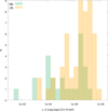 |
Fig. 11. Distribution of LX in the 0.5−10 keV band for the subsample of 77 BZBs with a well-determined redshift estimate reported in the Roma-BZCat (Massaro et al. 2015a). As in previous figures, LBLs are in orange and HBLs in green. |
5. Theoretical interpretation
The theoretical connection between synchrotron and IC processes in the SSC scenario has previosly been extensively investigated (see, e.g., Dermer 1995; Bloom & Marscher 1996; Mastichiadis & Kirk 1997; Dermer & Schlickeiser 2002; Massaro et al. 2006; Tramacere et al. 2011, and references therein). However, possible observable connections between X-ray and γ-ray emissions in BZBs are not yet fully exploited, certainly not on a statistical sample as we analyzed here.
As previously stated, while we carried out this investigation, we found that HBLs tend to be brighter in the X-rays than LBLs and cover a wider range of fluxes. On the other hand, LBLs cover a wide range of HRX, being generally harder than HBLs in the X-rays. These results suggest that on average HBLs do not vary their X-ray spectral shape significanlty, but only their total integrated power, and the opposite holds for LBLs.
According to the SSC scenario, we could interpret this as follows. For LBLs a decrease in synchrotron emission in the X-rays could be balanced by an increase in IC component. This implies a certain balance in the total X-ray flux, but a noticeable change in the spectral shape (i.e., X-ray hardness ratio HRX). On the other hand, the fact that for HBLs, HRX is restricted to a narrow range of values implies that the position of the synchrotron peak remains constant on average, and that we only observe the high-energy tail of their synchrotron component in X-rays.
We expect that the HBL behavior in X-rays is consistent with the theoretical scenario proposed in Massaro et al. (2011d) on the basis of the acceleration mechanism proposed by Cavaliere & Morrison (1980). Thus, assuming that the beaming factor of HBL jets does not vary significantly, as the total number of emitting particles, and following Paggi et al. (2009b), we state that the frequency of the synchrotron peak scales as  , where B is the average magnetic field in the emission region and γ3p is the peak of the γ n(γ), with n(γ) the particle energy distribution (see Tramacere et al. 2007, 2011, for details). For HBLs, νs remains constant on average, implying that
  . Assuming that the IC emission occurs in the Thomson regime, we expect that the SED peak frequency of the high-energy component scales as νic ∝ γ3p νs, thus as
  under the circumstances previously described. On the other hand, the peak height of the IC component being in general proportional to
  does not show significant changes if particle energy distribution and magnetic field are the main driver of spectral variations (Paggi et al. 2011).
According to Blandford & Znajek (1977) and Cavaliere & D’Elia (2002), the BZB luminosity should be limited by the Blandford−Znajek (BZ) limit (Ghosh & Abramowicz 1997; Tchekhovskoy et al. 2009), defined as  erg s−1, where MBH is the central black hole mass, and MSun the mass of the Sun. This condition applies only if the output can be ascribed solely to the black hole (i.e., in “dry” sources), which is a useful benchmark to analyze whether accretion is negligible in BZBs (Paggi et al. 2009a).
There is evidence, however, that BZBs might be emitting more than what can be described within this benchmark alone (see, e.g., Tavecchio & Ghisellini 2016). In presence of significant current accretion, we expect the jet launched from the central black hole to be more powerful (Ghisellini et al. 2014), and thus yielding higher observed luminosities that ultimately exceed the BZ limit, which instead applies to sources that are only powered by rotation.
For our sample we found 27 black hole mass estimates, measured with different methods as reported by Woo et al. (2005), Plotkin et al. (2011), León-Tavares et al. (2011); Sbarrato et al. (2012), Shaw et al. (2012), Xiong & Zhang (2014) and Ghisellini & Tavecchio (2015). We used them to compute the ratio of the sum of LX + Lγ to the BZ luminosity limit. LX was computed from our data in the 0.5−10 keV band, and Lγ was obtained in the 100 MeV−100 GeV band as listed in 3FGL. We adopted LX + Lγ as an estimate of the bolometric luminosity because at least one of them is close to the SED peak. Thus, we expect the ratio to be below 1 if the BZ limit is applicable. In Fig. 12 we plot this ratio versus the position of the rest-frame synchrotron peak taken from the 3FGL catalog.
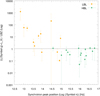 |
Fig. 12. Synchrotron peak frequency vs. the ratio between the estimate of the bolometric luminosity and the BZ luminosity, computed as reported in Sect. 5. As in previous figures, LBLs are in orange and HBLs in green. The gray dashed line indicates a luminosity ratio of 1, below which “dry” BZBs should lie. |
It is clear that all HBLs are still below the BZ limit, which is expected because they are the less bolometrically luminous type of blazar (Sambruna et al. 1996). In the LBL case, however, 8 out of 12 are above the BZ limit. Although the subsample is small, this is an indication that the BZ benchmark does not apply cleanly to the LBL scenario, as it does for HBLs.
An explanation for this discrepancy between the BZ benchmark and the observed LBL luminosities might be that these eight sources are probably not “dry” sources as HBLs. Thus their broadband emission is contaminated by IC scattering of seed photons arising from surrounding gas and/or the accretion disk (Abdo et al. 2015; Arsioli & Chang 2018). This is also consistent with the fact that LBLs are more similar to BZQs, and in these cases, the accretion component is important. In particular, for all these cases, Lγ is more than one order of magnitude higher than the X-ray luminosity, which is a strong indication that emission in these sources is strongly affected by an external Compton process (Arsioli & Chang 2018).
6. Summary and conclusions
We characterized the X-ray properties of Fermi BZBs, searching for a possible connection between X-rays and γ-raysthat could motivate follow-up X-ray observations to discover new blazar-like counterparts of UGSs (Stroh & Falcone 2013; Paggi et al. 2013; Massaro et al. 2015d). To achieve our goal, we built a sample of 351 BZBs listed by Fermi that were observed by the Swift/XRT telescope in photon-counting mode, with exposure times between 1 and 20 ks, and collected up to December 2018.
-
Of the 351 Fermi BZBs that were observed by XRT for more than 1 ks, 96% (337) were detected with an S/N > 3 (mean S/N of 25). We obtained accurate positions, counts, count rates, fluxes, and images for all of them in the soft X-ray band between 0.5 and 10 keV.
-
The BZBs are on average brighter in X-rays than other X-ray emitting sources that lie outside of the galactic plane (|b| > 10°). When they are classified as HBLs and LBLs, HBLs are generally brighter in X-ray flux and cover a wider range of flux values than LBLs.
-
On the other hand, the spectral shape of LBLs in X-rays is harder and less uniform than that of HBLs. This might be due to a more variable spectral shape in the X-ray band: for HBLs, the X-ray emission is dominated by the synchrotron process, while for LBLs the IC component is non-negligible.
-
We proved the direct link between the X-ray and γ-ray emission in BZBs, as supported by the high detection rate (96%) of their X-ray counterparts. This rate would remain unchanged even with shorter exposure times (5 ks).
-
The FX and mid-infrared color [4.6]−[12] μm (p < 1 × 10⁻⁷) are correlated. X-ray brighter BZBs are bluer in the mid-infrared.
-
For a subsample of 77 sources we obtained redshift values that allowed us to compute distances and luminosities. We note that HBLs are bolometrically less luminous than LBLs.
-
For 27 sources out of these 77 with a determined redshift, we also searched for values of the central black hole mass in the literature. All HBLs are below their BZ limit. However, some LBLs exceed this limit. We speculate that this indicates that LBLs may be accreting more gas than HBLs, meaning that the “dry” hypothesis would be valid only in the latter, not in the former.
5BZBJ 1046−2535 was not included because of light contamination from a nearby star. 5BZB J2108−6637 is the only source for which no WISE counterpart was found.
Acknowledgments
E. J. Marchesini would like to thank Rocío I. Páez and M. Victoria Reynaldi for useful discussions on this work. This work is supported by the “Departments of Excellence 2018−2022” Grant awarded by the Italian Ministry of Education, University and Research (MIUR) (L. 232/2016). This research has made use of resources provided by the Compagnia di San Paolo for the grant awarded on the BLENV project (S1618_L1_MASF_01) and by the Ministry of Education, Universities and Research for the grant MASF_FFABR_17_01. F. M. acknowledges financial contribution from the agreement ASI-INAF n.2017-14-H.0 A. P. acknowledges financial support from the Consorzio Interuniversitario per la fisica Spaziale (CIFS) under the agreement related to the grant MASF_CONTR_FIN_18_02. This research has made use of data obtained from the high- energy Astrophysics Science Archive Research Center (HEASARC) provided by NASA’s Goddard Space Flight Center. This work is part of a project that has received funding from the European Union’s Horizon 2020 Research and Innovation Programme under the Marie Słodowska-Curie Grant Agreement No. 664931. Part of this work is based on the NVSS (NRAO VLA Sky Survey). The National Radio Astronomy Observatory is operated by Associated Universities, Inc., under contract with the National Science Foundation. The Molonglo Observatory site manager, Duncan Campbell-Wilson, and the staff, Jeff Webb, Michael White, and John Barry, are responsible for the smooth operation of the Molonglo Observatory Synthesis Telescope (MOST) and the day-to-day observing program of SUMSS. SUMSS is dedicated to Michael Large, whose expertise and vision made the project possible. The MOST is operated by the School of Physics with the support of the Australian Research Council and the Science Foundation for Physics within the University of Sydney. This publication makes use of data products from the Wide-field Infrared Survey Explorer, which is a joint project of the University of California, Los Angeles, and the Jet Propulsion Laboratory/California Institute of Technology, funded by the National Aeronautics and Space Administration. TOPCAT (http://www.star.bris.ac.uk/~mbt/topcat/) (Taylor 2005) and STILTS (Taylor 2006) were used for the preparation and manipulation of the images and the tabular data.
References
- Abdo, A. A., Ackermann, M., Ajello, M., et al. 2015, ApJ, 799, 143 [NASA ADS] [CrossRef] [Google Scholar]
- Acero, F., Ackermann, M., Ajello, M., et al. 2015, ApJS, 218, 23 [Google Scholar]
- Ackermann, M., Ajello, M., Allafort, A., et al. 2011, ApJ, 741, 30 [NASA ADS] [CrossRef] [Google Scholar]
- Ackermann, M., Ajello, M., Atwood, W. B., et al. 2015, ApJ, 810, 14 [NASA ADS] [CrossRef] [Google Scholar]
- Aharonian, F., Akhperjanian, A. G., Aye, K.-M., et al. 2005, A&A, 436, L17 [NASA ADS] [CrossRef] [EDP Sciences] [Google Scholar]
- Albert, J., Aliu, E., Anderhub, H., et al. 2007, ApJ, 669, 862 [NASA ADS] [CrossRef] [Google Scholar]
- Álvarez Crespo, N., Masetti, N., Ricci, F., et al. 2016a, AJ, 151, 32 [NASA ADS] [CrossRef] [Google Scholar]
- Álvarez Crespo, N., Massaro, F., Milisavljevic, D., et al. 2016b, AJ, 151, 95 [NASA ADS] [CrossRef] [Google Scholar]
- Álvarez Crespo, N., Massaro, F., D’Abrusco, R., et al. 2016c, Ap&SS, 361, 316 [NASA ADS] [CrossRef] [Google Scholar]
- Arsioli, B., & Chang, Y. L. 2018, A&A, 616, A63 [NASA ADS] [CrossRef] [EDP Sciences] [Google Scholar]
- Banerjee, B., Joshi, M., Majumdar, P., et al. 2019, MNRAS, 487, 845 [NASA ADS] [CrossRef] [Google Scholar]
- Blandford, R. D., & Rees, M. J. 1978, in BL Lac Objects, ed. A. M. Wolfe, 328 [Google Scholar]
- Blandford, R. D., & Znajek, R. L. 1977, MNRAS, 179, 433 [NASA ADS] [CrossRef] [Google Scholar]
- Bloom, S. D. 2008, AJ, 136, 1533 [NASA ADS] [CrossRef] [Google Scholar]
- Bloom, S. D., & Marscher, A. P. 1996, ApJ, 461, 657 [NASA ADS] [CrossRef] [Google Scholar]
- Bondi, M., Marchã, M. J. M., Dallacasa, D., & Stanghellini, C. 2001, MNRAS, 325, 1109 [NASA ADS] [CrossRef] [Google Scholar]
- Böttcher, M., Basu, S., Joshi, M., et al. 2007, ApJ, 670, 968 [NASA ADS] [CrossRef] [Google Scholar]
- Brinkmann, W., Papadakis, I. E., Raeth, C., Mimica, P., & Haberl, F. 2005, A&A, 443, 397 [NASA ADS] [CrossRef] [EDP Sciences] [Google Scholar]
- Bruni, G., Panessa, F., Ghisellini, G., et al. 2018, ApJ, 854, L23 [NASA ADS] [CrossRef] [Google Scholar]
- Capalbi, M., Perri, M., Saija, B., & Tamburelli, F. 2005, ASI Science Data Center, 1 [Google Scholar]
- Carini, M. T., Miller, H. R., Noble, J. C., & Goodrich, B. D. 1992, AJ, 104, 15 [NASA ADS] [CrossRef] [Google Scholar]
- Cavaliere, A., & D’Elia, V. 2002, ApJ, 571, 226 [NASA ADS] [CrossRef] [Google Scholar]
- Cavaliere, A., & Morrison, P. 1980, ApJ, 238, L63 [NASA ADS] [CrossRef] [Google Scholar]
- Ciaramella, A., Bongardo, C., Aller, H. D., et al. 2004, A&A, 419, 485 [NASA ADS] [CrossRef] [EDP Sciences] [Google Scholar]
- Condon, J. J., Cotton, W. D., Greisen, E. W., et al. 1998, AJ, 115, 1693 [NASA ADS] [CrossRef] [Google Scholar]
- Cutini, S., Ciprini, S., Orienti, M., et al. 2014, MNRAS, 445, 4316 [NASA ADS] [CrossRef] [Google Scholar]
- D’Abrusco, R., Longo, G., & Walton, N. A. 2009, MNRAS, 396, 223 [NASA ADS] [CrossRef] [Google Scholar]
- D’Abrusco, R., Massaro, F., Ajello, M., et al. 2012, ApJ, 748, 68 [NASA ADS] [CrossRef] [Google Scholar]
- D’Abrusco, R., Massaro, F., Paggi, A., et al. 2013, ApJS, 206, 12 [NASA ADS] [CrossRef] [Google Scholar]
- D’Abrusco, R., Massaro, F., Paggi, A., et al. 2014, ApJS, 215, 14 [NASA ADS] [CrossRef] [Google Scholar]
- D’Elia, V., Perri, M., Puccetti, S., et al. 2013, A&A, 551, A142 [NASA ADS] [CrossRef] [EDP Sciences] [Google Scholar]
- Dermer, C. D. 1995, ApJ, 446, L63 [NASA ADS] [CrossRef] [Google Scholar]
- Dermer, C. D., & Schlickeiser, R. 2002, ApJ, 575, 667 [NASA ADS] [CrossRef] [Google Scholar]
- D’Abrusco, R., Álvarez Crespo, N., Massaro, F., et al. 2019, ApJS, 242, 4 [NASA ADS] [CrossRef] [Google Scholar]
- Dunkley, J., Komatsu, E., Nolta, M. R., et al. 2009, ApJS, 180, 306 [NASA ADS] [CrossRef] [Google Scholar]
- Evans, P. A., Osborne, J. P., Beardmore, A. P., et al. 2014, ApJS, 210, 8 [NASA ADS] [CrossRef] [Google Scholar]
- Falcone, A. 2013, AAS/High Energy Astrophysics Division, 13, 114.07 [NASA ADS] [Google Scholar]
- Falcone, A., Stroh, M., & Pryal, M. 2014, Am. Astron. Soc. Meet. Abstr., 223, 301.05 [NASA ADS] [Google Scholar]
- Fermi-LAT Collaboration 2019, ApJS, submitted [arXiv:1902.10045] [Google Scholar]
- Fichtel, C. E., Bertsch, D. L., Dingus, B., et al. 1993, Adv. Space Res., 13, 637 [NASA ADS] [CrossRef] [Google Scholar]
- Finke, J. D., Dermer, C. D., & Böttcher, M. 2008, ApJ, 686, 181 [NASA ADS] [CrossRef] [Google Scholar]
- Ghirlanda, G., Ghisellini, G., Tavecchio, F., & Foschini, L. 2010, MNRAS, 407, 791 [NASA ADS] [CrossRef] [Google Scholar]
- Ghirlanda, G., Ghisellini, G., Tavecchio, F., Foschini, L., & Bonnoli, G. 2011, MNRAS, 413, 852 [NASA ADS] [CrossRef] [Google Scholar]
- Ghisellini, G., & Tavecchio, F. 2015, MNRAS, 448, 1060 [NASA ADS] [CrossRef] [Google Scholar]
- Ghisellini, G., Maraschi, L., & Treves, A. 1985, A&A, 146, 204 [NASA ADS] [Google Scholar]
- Ghisellini, G., Tavecchio, F., Foschini, L., et al. 2010, MNRAS, 402, 497 [NASA ADS] [CrossRef] [Google Scholar]
- Ghisellini, G., Tavecchio, F., Maraschi, L., Celotti, A., & Sbarrato, T. 2014, Nature, 515, 376 [NASA ADS] [CrossRef] [Google Scholar]
- Ghisellini, G., Righi, C., Costamante, L., & Tavecchio, F. 2017, MNRAS, 469, 255 [NASA ADS] [CrossRef] [Google Scholar]
- Ghosh, P., & Abramowicz, M. A. 1997, MNRAS, 292, 887 [NASA ADS] [CrossRef] [Google Scholar]
- Giannios, D., Uzdensky, D. A., & Begelman, M. C. 2009, MNRAS, 395, L29 [NASA ADS] [CrossRef] [Google Scholar]
- Giommi, P., Barr, P., Garilli, B., Maccagni, D., & Pollock, A. M. T. 1990, ApJ, 356, 432 [NASA ADS] [CrossRef] [Google Scholar]
- Giroletti, M., Massaro, F., D’Abrusco, R., et al. 2016, A&A, 588, A141 [NASA ADS] [CrossRef] [EDP Sciences] [Google Scholar]
- Hartman, R. C., Bertsch, D. L., Bloom, S. D., et al. 1999, ApJS, 123, 79 [NASA ADS] [CrossRef] [Google Scholar]
- Hartman, R. C., Böttcher, M., Aldering, G., et al. 2001, ApJ, 553, 683 [NASA ADS] [CrossRef] [Google Scholar]
- Healey, S. E., Romani, R. W., Taylor, G. B., et al. 2007, ApJS, 171, 61 [NASA ADS] [CrossRef] [Google Scholar]
- Hervet, O., Williams, D. A., Falcone, A. D., & Kaur, A. 2019, ApJ, 877, 26 [NASA ADS] [CrossRef] [Google Scholar]
- Impey, C. D., & Neugebauer, G. 1988, AJ, 95, 307 [NASA ADS] [CrossRef] [Google Scholar]
- Isobe, N., Sugimori, K., Kawai, N., et al. 2010, PASJ, 62, L55 [NASA ADS] [Google Scholar]
- Jorstad, S. G., Marscher, A. P., Mattox, J. R., et al. 2001, ApJS, 134, 181 [NASA ADS] [CrossRef] [Google Scholar]
- Kalberla, P. M. W., Burton, W. B., Hartmann, D., et al. 2005, A&A, 440, 775 [NASA ADS] [CrossRef] [EDP Sciences] [Google Scholar]
- Kataoka, J., Yatsu, Y., Kawai, N., et al. 2012, ApJ, 757, 176 [NASA ADS] [CrossRef] [Google Scholar]
- Kaur, N., Chandra, S., Baliyan, K. S., & Ganesh, S. 2017, ApJ, 846, 158 [NASA ADS] [CrossRef] [Google Scholar]
- Landi, R., Bassani, L., Stephen, J. B., et al. 2015, A&A, 581, A57 [NASA ADS] [CrossRef] [EDP Sciences] [Google Scholar]
- Landoni, M., Massaro, F., Paggi, A., et al. 2015, AJ, 149, 163 [NASA ADS] [CrossRef] [Google Scholar]
- Laurino, O., D’Abrusco, R., Longo, G., & Riccio, G. 2011, MNRAS, 418, 2165 [NASA ADS] [CrossRef] [Google Scholar]
- León-Tavares, J., Valtaoja, E., Chavushyan, V. H., et al. 2011, MNRAS, 411, 1127 [NASA ADS] [CrossRef] [Google Scholar]
- Lico, R., Giroletti, M., Orienti, M., et al. 2014, A&A, 571, A54 [NASA ADS] [CrossRef] [EDP Sciences] [Google Scholar]
- Lister, M. L., Aller, M. F., Aller, H. D., et al. 2013, AJ, 146, 120 [NASA ADS] [CrossRef] [Google Scholar]
- Lister, M. L., Homan, D. C., Hovatta, T., et al. 2019, ApJ, 874, 43 [NASA ADS] [CrossRef] [Google Scholar]
- Mahony, E. K., Sadler, E. M., Murphy, T., et al. 2010, ApJ, 718, 587 [NASA ADS] [CrossRef] [Google Scholar]
- Mao, P., Urry, C. M., Massaro, F., et al. 2016, ApJS, 224, 26 [NASA ADS] [CrossRef] [Google Scholar]
- Maraschi, L., Ghisellini, G., & Celotti, A. 1992, ApJ, 397, L5 [NASA ADS] [CrossRef] [Google Scholar]
- Marchesini, E. J., Masetti, N., Chavushyan, V., et al. 2016, A&A, 596, A10 [NASA ADS] [CrossRef] [EDP Sciences] [Google Scholar]
- Marchesini, E. J., Peña-Herazo, H. A., Álvarez Crespo, N., et al. 2019a, Ap&SS, 364, 5 [NASA ADS] [CrossRef] [Google Scholar]
- Marchesini, E. J., Peña-Herazo, H. A., Álvarez Crespo, N., et al. 2019b, Ap&SS, 364, 5 [NASA ADS] [CrossRef] [Google Scholar]
- Maselli, A., Massaro, E., Nesci, R., et al. 2010, A&A, 512, A74 [NASA ADS] [CrossRef] [EDP Sciences] [Google Scholar]
- Maselli, A., Massaro, F., Cusumano, G., et al. 2013, ApJS, 206, 17 [NASA ADS] [CrossRef] [Google Scholar]
- Masetti, N., Sbarufatti, B., Parisi, P., et al. 2013, A&A, 559, A58 [NASA ADS] [CrossRef] [EDP Sciences] [Google Scholar]
- Massaro, F., & D’Abrusco, R. 2016, ApJ, 827, 67 [NASA ADS] [CrossRef] [Google Scholar]
- Massaro, E., Tramacere, A., Perri, M., Giommi, P., & Tosti, G. 2006, A&A, 448, 861 [NASA ADS] [CrossRef] [EDP Sciences] [Google Scholar]
- Massaro, F., Tramacere, A., Cavaliere, A., Perri, M., & Giommi, P. 2008a, A&A, 478, 395 [NASA ADS] [CrossRef] [EDP Sciences] [Google Scholar]
- Massaro, F., Giommi, P., Tosti, G., et al. 2008b, A&A, 489, 1047 [NASA ADS] [CrossRef] [EDP Sciences] [Google Scholar]
- Massaro, F., D’Abrusco, R., Ajello, M., Grindlay, J. E., & Smith, H. A. 2011a, ApJ, 740, L48 [NASA ADS] [CrossRef] [Google Scholar]
- Massaro, F., Paggi, A., Elvis, M., & Cavaliere, A. 2011b, ApJ, 739, 73 [NASA ADS] [CrossRef] [Google Scholar]
- Massaro, F., Harris, D. E., & Cheung, C. C. 2011c, ApJS, 197, 24 [NASA ADS] [CrossRef] [Google Scholar]
- Massaro, F., Paggi, A., & Cavaliere, A. 2011d, ApJ, 742, L32 [NASA ADS] [CrossRef] [Google Scholar]
- Massaro, F., D’Abrusco, R., Tosti, G., et al. 2012a, ApJ, 750, 138 [NASA ADS] [CrossRef] [Google Scholar]
- Massaro, F., D’Abrusco, R., Tosti, G., et al. 2012b, ApJ, 752, 61 [NASA ADS] [CrossRef] [Google Scholar]
- Massaro, F., Tremblay, G. R., Harris, D. E., et al. 2012c, ApJS, 203, 31 [NASA ADS] [CrossRef] [Google Scholar]
- Massaro, F., D’Abrusco, R., Giroletti, M., et al. 2013a, ApJS, 207, 4 [NASA ADS] [CrossRef] [Google Scholar]
- Massaro, F., Paggi, A., Errando, M., et al. 2013b, ApJS, 207, 16 [NASA ADS] [CrossRef] [Google Scholar]
- Massaro, F., D’Abrusco, R., Paggi, A., et al. 2013c, ApJS, 209, 10 [NASA ADS] [CrossRef] [Google Scholar]
- Massaro, F., Giroletti, M., Paggi, A., et al. 2013d, ApJS, 208, 15 [NASA ADS] [CrossRef] [Google Scholar]
- Massaro, F., Masetti, N., D’Abrusco, R., Paggi, A., & Funk, S. 2014, AJ, 148, 66 [NASA ADS] [CrossRef] [Google Scholar]
- Massaro, E., Maselli, A., Leto, C., et al. 2015a, Ap&SS, 357, 75 [NASA ADS] [CrossRef] [Google Scholar]
- Massaro, F., Thompson, D. J., & Ferrara, E. C. 2015b, A&ARv, 24, 2 [NASA ADS] [CrossRef] [Google Scholar]
- Massaro, F., Landoni, M., D’Abrusco, R., et al. 2015c, A&A, 575, A124 [NASA ADS] [CrossRef] [EDP Sciences] [Google Scholar]
- Massaro, F., D’Abrusco, R., Landoni, M., et al. 2015d, ApJS, 217, 2 [NASA ADS] [CrossRef] [Google Scholar]
- Massaro, F., Álvarez Crespo, N., D’Abrusco, R., et al. 2016, Ap&SS, 361, 337 [NASA ADS] [CrossRef] [Google Scholar]
- Mastichiadis, A., & Kirk, J. G. 1997, A&A, 320, 19 [NASA ADS] [Google Scholar]
- Mattox, J. R., & Ormes, J. F. 2002, Am. Astron. Soc. Meet. Abstr., 201, 147.02 [NASA ADS] [Google Scholar]
- Mauch, T., Murphy, T., Buttery, H. J., et al. 2003, MNRAS, 342, 1117 [NASA ADS] [CrossRef] [Google Scholar]
- Mirabal, N. 2009, ArXiv e-prints [arXiv:0908.1389] [Google Scholar]
- Moretti, A., Campana, S., Tagliaferri, G., et al. 2004, in X-Ray and Gamma-Ray Instrumentation for Astronomy XIII, eds. K. A. Flanagan, & O. H. W. Siegmund, Proc. SPIE, 5165, 232 [NASA ADS] [CrossRef] [Google Scholar]
- Mukai, K. 1993, Legacy, 3, 21 [Google Scholar]
- Nori, M., Giroletti, M., Massaro, F., et al. 2014, ApJS, 212, 3 [NASA ADS] [CrossRef] [Google Scholar]
- Paggi, A., Cavaliere, A., Vittorini, V., & Tavani, M. 2009a, A&A, 508, L31 [NASA ADS] [CrossRef] [EDP Sciences] [Google Scholar]
- Paggi, A., Massaro, F., Vittorini, V., et al. 2009b, A&A, 504, 821 [NASA ADS] [CrossRef] [EDP Sciences] [Google Scholar]
- Paggi, A., Cavaliere, A., Vittorini, V., D’Ammando, F., & Tavani, M. 2011, ApJ, 736, 128 [NASA ADS] [CrossRef] [Google Scholar]
- Paggi, A., Massaro, F., D’Abrusco, R., et al. 2013, ApJS, 209, 9 [NASA ADS] [CrossRef] [Google Scholar]
- Paggi, A., Milisavljevic, D., Masetti, N., et al. 2014, AJ, 147, 112 [NASA ADS] [CrossRef] [Google Scholar]
- Paiano, S., Franceschini, A., & Stamerra, A. 2017, MNRAS, 468, 4902 [NASA ADS] [CrossRef] [Google Scholar]
- Pandey, A., Gupta, A. C., & Wiita, P. J. 2017, ApJ, 841, 123 [NASA ADS] [CrossRef] [Google Scholar]
- Peña-Herazo, H. A., Marchesini, E. J., Álvarez Crespo, N., et al. 2017a, Ap&SS, 362, 228 [NASA ADS] [CrossRef] [Google Scholar]
- Peña-Herazo, H. A., Marchesini, E. J., Álvarez Crespo, N., et al. 2017b, Ap&SS, 362, 228 [NASA ADS] [CrossRef] [Google Scholar]
- Peña-Herazo, H. A., Massaro, F., Chavushyan, V., et al. 2019, Ap&SS, 364, 85 [NASA ADS] [CrossRef] [Google Scholar]
- Pian, E., Vacanti, G., Tagliaferri, G., et al. 1998, ApJ, 492, L17 [NASA ADS] [CrossRef] [Google Scholar]
- Piner, B. G., & Edwards, P. G. 2014, ApJ, 797, 25 [NASA ADS] [CrossRef] [Google Scholar]
- Piner, B. G., & Edwards, P. G. 2018, ApJ, 853, 68 [NASA ADS] [CrossRef] [Google Scholar]
- Plotkin, R. M., Markoff, S., Trager, S. C., & Anderson, S. F. 2011, MNRAS, 413, 805 [NASA ADS] [CrossRef] [Google Scholar]
- Ricci, F., Massaro, F., Landoni, M., et al. 2015, AJ, 149, 160 [NASA ADS] [CrossRef] [Google Scholar]
- Romero, G. E., Cellone, S. A., Combi, J. A., & Andruchow, I. 2002, A&A, 390, 431 [NASA ADS] [CrossRef] [EDP Sciences] [Google Scholar]
- Sambruna, R. M., Maraschi, L., & Urry, C. M. 1996, ApJ, 463, 444 [NASA ADS] [CrossRef] [Google Scholar]
- Sbarrato, T., Ghisellini, G., Maraschi, L., & Colpi, M. 2012, MNRAS, 421, 1764 [NASA ADS] [CrossRef] [Google Scholar]
- Shaw, M. S., Romani, R. W., Cotter, G., et al. 2012, ApJ, 748, 49 [CrossRef] [Google Scholar]
- Sikora, M., Janiak, M., Nalewajko, K., Madejski, G. M., & Moderski, R. 2013, ApJ, 779, 68 [NASA ADS] [CrossRef] [Google Scholar]
- Singh, K. P., & Garmire, G. P. 1985, ApJ, 297, 199 [NASA ADS] [CrossRef] [Google Scholar]
- Stecker, F. W., Salamon, M. H., & Malkan, M. A. 1993, ApJ, 410, L71 [NASA ADS] [CrossRef] [Google Scholar]
- Stevens, J. A., Litchfield, S. J., Robson, E. I., et al. 1994, ApJ, 437, 91 [NASA ADS] [CrossRef] [Google Scholar]
- Stickel, M., Padovani, P., Urry, C. M., Fried, J. W., & Kuehr, H. 1991, ApJ, 374, 431 [NASA ADS] [CrossRef] [Google Scholar]
- Stroh, M. C., & Falcone, A. D. 2013, ApJS, 207, 28 [NASA ADS] [CrossRef] [Google Scholar]
- Tavecchio, F., & Ghisellini, G. 2016, MNRAS, 456, 2374 [NASA ADS] [CrossRef] [Google Scholar]
- Tavecchio, F., Ghisellini, G., Bonnoli, G., & Foschini, L. 2011, MNRAS, 414, 3566 [NASA ADS] [CrossRef] [Google Scholar]
- Taylor, M. B. 2005, in Astronomical Data Analysis Software and Systems XIV, eds. P. Shopbell, M. Britton, & R. Ebert, ASP Conf. Ser., 347, 29 [Google Scholar]
- Taylor, M. B. 2006, in Astronomical Data Analysis Software and Systems XV, eds. C. Gabriel, C. Arviset, D. Ponz, & S. Enrique, ASP Conf. Ser., 351, 666 [Google Scholar]
- Taylor, G. B., Healey, S. E., Helmboldt, J. F., et al. 2007, ApJ, 671, 1355 [NASA ADS] [CrossRef] [Google Scholar]
- Tchekhovskoy, A., McKinney, J. C., & Narayan, R. 2009, ApJ, 699, 1789 [NASA ADS] [CrossRef] [Google Scholar]
- Tramacere, A., Massaro, F., & Cavaliere, A. 2007, A&A, 466, 521 [NASA ADS] [CrossRef] [EDP Sciences] [Google Scholar]
- Tramacere, A., Massaro, E., & Taylor, A. M. 2011, ApJ, 739, 66 [NASA ADS] [CrossRef] [Google Scholar]
- Voges, W., Aschenbach, B., Boller, T., et al. 1999, A&A, 349, 389 [NASA ADS] [Google Scholar]
- Wehrle, A. E., Pian, E., Urry, C. M., et al. 1998, ApJ, 497, 178 [NASA ADS] [CrossRef] [Google Scholar]
- White, R. L., Becker, R. H., Helfand, D. J., & Gregg, M. D. 1997, ApJ, 475, 479 [NASA ADS] [CrossRef] [Google Scholar]
- Woo, J.-H., Urry, C. M., van der Marel, R. P., Lira, P., & Maza, J. 2005, ApJ, 631, 762 [NASA ADS] [CrossRef] [Google Scholar]
- Wright, E. L., Eisenhardt, P. R. M., Mainzer, A. K., et al. 2010, AJ, 140, 1868 [NASA ADS] [CrossRef] [Google Scholar]
- Xiong, D. R., & Zhang, X. 2014, MNRAS, 441, 3375 [NASA ADS] [CrossRef] [Google Scholar]
Appendix A: Complementary X-ray and mid-infrared combined figures
In Fig. A.1 we show the X-ray full-band flux versus the magnitudes at 3.4 and 4.6 μm from the AllWISE catalog in the upper and lower panel, respectively. They do not differ from the results in the main text, as shown in Fig. 10. In the same way, we show in Fig. A.2 the comparison between the X-ray full-band flux and the color index [3.4]−[4.6], which is comparable to Fig. 11. Finally, in Fig. A.3 we show the X-ray hardness ratio versus the color index [3.4]−[4.6], which follows the same trend as discussed for Fig. 10.
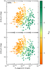 |
Fig. A.1. FX in the 0.5−10 keV band vs. the WISE magnitude estimate at a nominal wavelength of 3.4 μm (upper panel) and vs. that evaluated at 4.6 μm (lower panel). BZBs classified as LBL are shown in orange and HBLs are marked in green. |
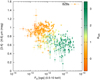 |
Fig. A.2. FX in the 0.5−10 keV band vs. the [3.4]−[4.6] μm mid-infrared color. |
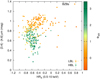 |
Fig. A.3. HRX in the 0.5−10 keV band vs. the [3.4]−[4.6] μm. Average uncertainties on these two parameters are shown as crosses in the bottom right corner. |
All Tables
All Figures
|
Fig. 1. X-ray image in the 0.5−10 keV energy range obtained by merging all XRT observations within 6 arcmin measured from the γ-ray position of 5BZB J2005+7752 (left panel) and its corresponding merged exposure map (right panel). The bright source in the center is the X-ray counterpart of the BZB, marked with the white circle as all other background and foreground X-ray sources. This X-ray image has been built by merging five observations for an exposure time of 15.9 ks. The image is also smoothed with a Gaussian kernel with a radius of 5 pixels. |
| In the text | |
|
Fig. 2. Distribution of the total exposure time for all selected BZBs. The blue histogram indicates the X-ray merged event files with at least one X-ray source detected with an S/N > 3, while in red we show those without an X-ray detection. |
| In the text | |
|
Fig. 3. Flow chart to highlight all steps we followed to build our final BZBs sample. |
| In the text | |
|
Fig. 4. Distribution of Fγ in the 100 MeV−100 GeV band for all 351 BZBs in our selected sample. As in Fig. 2, the blue histogram indicates the X-ray merged event file with at least one X-ray source detected with S/N > 3, and in red we show those without an X-ray detection. The solid black line corresponds to the threshold above which 100% of the selected BZBs has an X-ray counterpart, while the dashed and dot-dashed black lines mark the 98% and 96% thresholds, respectively. |
| In the text | |
|
Fig. 5. FX in the 0.5−10 keV band vs. HRX for all BZBs in the selected sample. Background or foreground X-ray sources are marked in gray, and BZB classified as HBL and as LBL are marked in green and orange, respectively. The solid black line separates BZBs with pile-up, which show FX > 2.0 × 10⁻¹¹ erg cm−2 s−1. |
| In the text | |
|
Fig. 6. FX in the 0.5−10 keV band vs. HRX for all BZBs in the selected sample, same as in Fig. 5. We show the 70%, 80%, and 90% isodensity contours as obtained from a KDE analysis for background or foreground sources in gray, HBLs in green, and LBLs in orange. |
| In the text | |
|
Fig. 7. Angular separation between the X-ray and γ-ray position for all BZBs, in arcminutes. As in Fig. 5, BZBs classified as HBLs and LBLs are shown in green and orange, respectively, while background or foreground X-ray sources are shown in gray. |
| In the text | |
|
Fig. 8. Lower panel: FX in the 0.5−10 keV band vs. the WISE magnitude at 12 μm for all selected BZBs. Upper panel: FX in the 0.5−10 keV band vs. the Fγ in the 100 MeV−100 GeV band, collected from the 3FGL. BL Lac objects classified as HBLs and LBLs are shown in green and orange, respectively. |
| In the text | |
|
Fig. 9. Upper panel: FX in the 0.5−10 keV band vs. the [4.6]−[12] μm mid-infrared color. Selected BZBs are classified as HBLs and LBLs and are marked in green and orange, respectively. Dashed lines indicate regression lines for LBLs (purple), HBLs (red), and the whole sample (black). Lower panel: FX in the 0.5−10 keV band vs. the αγ as reported in the 3FGL. Solid black lines mark the area within one standard deviation centered on the mean, and solid gray shows the area computed with the median absolute deviation centered on the median value. |
| In the text | |
|
Fig. 10. Comparison of the spectral shape for all the BZBs in our sample. LBLs are shown in orange and HBLs in green. Upper panel: HRX in the 0.5−10 keV band vs. the [4.6]−[12] μm mid-infrared color. Lower panel: HRX in the 0.5−10 keV band vs. αγ. In both panels the average uncertainties on the parameters are shown as crosses in the top right corner. |
| In the text | |
|
Fig. 11. Distribution of LX in the 0.5−10 keV band for the subsample of 77 BZBs with a well-determined redshift estimate reported in the Roma-BZCat (Massaro et al. 2015a). As in previous figures, LBLs are in orange and HBLs in green. |
| In the text | |
|
Fig. 12. Synchrotron peak frequency vs. the ratio between the estimate of the bolometric luminosity and the BZ luminosity, computed as reported in Sect. 5. As in previous figures, LBLs are in orange and HBLs in green. The gray dashed line indicates a luminosity ratio of 1, below which “dry” BZBs should lie. |
| In the text | |
|
Fig. A.1. FX in the 0.5−10 keV band vs. the WISE magnitude estimate at a nominal wavelength of 3.4 μm (upper panel) and vs. that evaluated at 4.6 μm (lower panel). BZBs classified as LBL are shown in orange and HBLs are marked in green. |
| In the text | |
|
Fig. A.2. FX in the 0.5−10 keV band vs. the [3.4]−[4.6] μm mid-infrared color. |
| In the text | |
|
Fig. A.3. HRX in the 0.5−10 keV band vs. the [3.4]−[4.6] μm. Average uncertainties on these two parameters are shown as crosses in the bottom right corner. |
| In the text | |
Current usage metrics show cumulative count of Article Views (full-text article views including HTML views, PDF and ePub downloads, according to the available data) and Abstracts Views on Vision4Press platform.
Data correspond to usage on the plateform after 2015. The current usage metrics is available 48-96 hours after online publication and is updated daily on week days.
Initial download of the metrics may take a while.