| Issue |
A&A
Volume 631, November 2019
|
|
|---|---|---|
| Article Number | A174 | |
| Number of page(s) | 10 | |
| Section | Planets and planetary systems | |
| DOI | https://doi.org/10.1051/0004-6361/201936004 | |
| Published online | 19 November 2019 | |
Polarisation of a small-scale cometary plasma environment
Particle-in-cell modelling of comet 67P/Churyumov-Gerasimenko
1
Department of Physics, Umeå University,
901 87
Umeå,
Sweden
e-mail: herbert.gunell@physics.org
2
Royal Belgian Institute for Space Aeronomy (BIRA-IASB),
Avenue Circulaire 3,
1180
Brussels,
Belgium
3
Institut für Geophysik und extraterrestrische Physik, TU Braunschweig,
Mendelssohnstr. 3,
38106
Braunschweig,
Germany
4
Swedish Institute of Space Physics,
Box 812,
981 28
Kiruna,
Sweden
Received:
3
June
2019
Accepted:
24
October
2019
Context. The plasma near the nucleus of a comet is subjected to an electric field to which a few different sources contribute: the convective electric field of the solar wind, the ambipolar electric field due to higher electron than ion speeds, and a polarisation field arising from the vastly different ion and electron trajectories.
Aims. Our aim is to show how the ambipolar and polarisation electric fields arise and develop under the influence of space charge effects, and in doing so we paint a qualitative picture of the electric fields in the inner coma of a comet.
Methods. We use an electrostatic particle-in-cell model to simulate a scaled-down comet, representing comet 67P/Churyumov-Gerasimenko with parameters corresponding to a 3.0 AU heliocentric distance.
Results. We find that an ambipolar electric field develops early in the simulation and that this is soon followed by the emergence of a polarisation electric field, manifesting itself as an anti-sunward component prevalent in the region surrounding the centre of the comet. As plasma is removed from the inner coma in the direction of the convectional electric field of the solar wind, a density maximum develops on the opposite side of the centre of the comet.
Conclusions. The ambipolar and polarisation electric fields both have a significant influence on the motion of cometary ions. This demonstrates the importance of space charge effects in comet plasma physics.
Key words: comets: general / comets: individual: 67P/Churyumov-Gerasimenko / plasmas / acceleration of particles
© ESO 2019
1 Introduction
The comet–solar wind interaction goes through a number of different regimes as a comet approaches the sun, leading to increased outgassing from the nucleus and increased ionisation by solar extreme-UV (EUV) radiation. Similarly, the difference in outgassing rates between different comets affects the ways in which they interact with the solar wind. This difference is largely one of scale. The more actively outgassing comets have larger ion comae, both in absolute numbers and relative to characteristic length scales of the plasma, such as the Debye length and the gyroradii of electrons and ions. Thus, more ion velocity space diffusion was observed at comet 1P/Halley than at the much smaller 26P/Grigg-Skjellerup, which were both visited by the Giotto spacecraft in fast flybys (Johnstone et al. 1993). The present paper treats comet–solar wind interaction at weakly outgassing, and hence small-scale, comets and in particular comet 67P/Churyumov-Gerasimenko (67P) that was accompanied by the Rosetta spacecraft for two years (Glassmeier et al. 2007a). However, highly active comets also go through a weakly outgassing phase when they are far away from the Sun, and in the inner coma of a large-scale comet, small-scale phenomena may still be important.
During the first two months after Rosetta’s arrival at comet 67P in August 2014, when it was between 3.6 and 3.3 AU from the Sun, the interaction between the solar wind and the comet was dominated by weak mass loading (Nilsson et al. 2015a). Water group pick-up ions were observed as they were being accelerated by the solar wind electric field, and the solar wind protons were seen to be deflected by about 20°, but they were otherwise generally unaffected by the presence of the comet. Closer to the Sun, Rosetta observed the infant bow shock, that is to say a bow shock during its formation (Gunell et al. 2018). Then, when comet 67P was less than 1.8 AU from the Sun, no solar wind ions could be detected at all at the spacecraft position (Nilsson et al. 2017). The existence of several boundaries that could have formed upstream and whether they are transient or permanent features were the subjects of some discussions after the flybys of comet 1P/Halley (see e.g. Coates & Jones 2009; Mandt et al. 2016; Simon Wedlund et al. 2017).
The disappearance of the solar wind more or less coincided (to within 0.05 AU heliocentric distance) with the first detections of the diamagnetic cavity (Goetz et al. 2016a,b). Thus, another boundary had formed in the inner coma, separating an unmagnetised plasma near the nucleus from the magnetised plasma farther out. Wave activity in both the ion acoustic and lower hybrid frequency ranges has been reported in the vicinity of this boundary (e.g. Karlsson et al. 2017; Gunell et al. 2017; Madsen et al. 2018).
Hybrid simulations have shown that at comet 67P the gyroradius of the cometary water group pick-up ions is thousands of kilometres (e.g. Koenders et al. 2013; Gunell et al. 2015; Simon Wedlund et al. 2017), which is not only much larger than the electron gyroradius1, but also of the same order or larger than the whole comet–solar wind interaction region. As a particular example, Simon Wedlund et al. (2017) estimated the gyroradius to 1.5 − 2 × 10⁴ km for comet 67P at 1.3 AU and the bow shock standoff distance to about 7 × 10³ km. As a comet is immersed in the solar wind, this means that, on scales the size of the interaction region, newly born cometary ions will move in the direction of the convective electric field of the solar wind, while electrons will move at E ×B velocity. The situation is similar at other unmagnetised bodies such as Mars (Kallio & Jarvinen 2012) and Ceres (Lindkvist et al. 2017). The electron temperature during the low-activity phase of comet 67P in late 2014, after Rosetta’s arrival, was in the 5− 10 eV range. The plasma electrons dominated the spacecraft charging over photoemission from the spacecraft body, making the spacecraft potential negative with respect to the plasma (Odelstad et al. 2015; Eriksson et al. 2017). During this period “singing comet” waves were found at low frequencies, peaking at about 40 mHz (Richter et al. 2015, 2016), and were interpreted as a modified ion-Weibel instability (Meier et al. 2016).
The CRIT I rocket experiment conducted in 1986 shares important properties with a low-activity comet. In the CRIT I experiment, a barium plasma cloud was injected into Earth’s ionosphere with a significant velocity component perpendicular to the ambient magnetic field. As a comet moves relative to the magnetised solar wind, the barium plasma cloud moves relative to the magnetised plasma that is Earth’s ionosphere. Brenning et al. (1991) modelled the barium cloud using a cylindrical approximation of its shape. While the ions move in the electric field direction, the electrons E ×B drift in a direction perpendicular to it. This creates a charge separation, leading to a polarisation electric field, which in the cylindrical approximation is constant inside the cylinder and approximates a two-dimensional dipole field outside it (Herlofson 1951; Tonks 1931). When this field is superimposed on the convective electric field, the direction of the total electric field changes, changing the directions of the ion and electron velocities in the process. This leads to an oscillation, which was observed by Brenning et al. (1991). At a comet the direction of the convective electric field is fixed by the solar wind direction, and instead of an oscillation the total electric field is directed at an angle off the −u0 ×B0 direction, where u0 and B0 are the solar wind velocity and magnetic field, respectively (Nilsson et al. 2018).
In addition to the convectional and polarisation fields there is a third important contribution to the electric field in the inner coma of a comet, namely the ambipolar field. Most of the excess energy carried by the ionising solar EUV photons is assumed by the kinetic energy of the electrons. Therefore, the thermal speed of the electrons allows them to leave the inner coma faster than the ions, creating an electric field directed radially outward. Vigren & Eriksson (2017) modelled the motion of ions in the coma, under the influence of the ambipolar electric field, and found that the ions are not collisionally coupled to the neutrals, and that the relative ion–neutral velocity can reach several km s−1. This result was confirmed experimentally by Odelstad et al. (2018) using Langmuir probe measurements. The work on the ambipolar field by Vigren & Eriksson (2017) and Odelstad et al. (2018) was performed for comet 67P close to perihelion. However, Beth & Galand (2018) found that also in the low-activity case the ions move faster than the neutrals, due in part to the ambipolar electric field, but also to the convective electric field.
The polarisation of a comet ionosphere is similar to laboratory experiments with plasmoids encountering magnetic barriers and to magnetosheath plasmoids (also known as jets) interacting with Earth’s magnetopause (Plaschke et al. 2018). In laboratory experiments on plasmoids encountering magnetic barriers, polarisation electric fields have been seen to form, allowing the plasmoid to convect into the downstream region of the barrier (Hurtig et al. 2004; Brenning et al. 2005). Electrostatic particle-in-cell simulations of these experiments could reproduce the behaviour of the laboratory plasma including both polarisation and generation of waves in the lower hybrid frequency range (Hurtig et al. 2003; Gunell et al. 2008, 2009). In space, plasmoids penetrating the magnetopause have been observed by the Cluster spacecraft (Gunell et al. 2012). The conditions for a plasmoid to pass through a tangential discontinuity has been studied in detail in a series of articles, using electromagnetic particle-in-cell simulations (Voitcu & Echim 2016, 2017, 2018).
In this paper we report results of an electrostatic particle-in-cell simulation that paints a qualitative picture of the electric fields in the ionised coma of a scaled-down version of comet 67P. The present simulation follows the same principles as the simulations of plasmoids encountering magnetic barriers, but it is designed to emulate the conditions of a comet in the solar wind.
2 Model
We use an electrostatic particle-in-cell model called Picard to simulate the interaction between comet 67P and the solar wind plasma (Lindkvist & Gunell 2019). It is a standard three-dimensional particle-in-cell code of the kind described by Hockney & Eastwood (1988) or Birdsall & Langdon (1991), among others. Following previous simulations of a similar problem (Hurtig et al. 2003; Hurtig 2004; Gunell et al. 2008, 2009) we use open boundary conditions. This means that we assume that the space outside the simulation box is empty; we compute the potential that the charges inside the simulation box give rise to on the boundaries of that box, and then these potentials are used as a Dirichlet boundary condition for Poisson’s equation. We solve Poisson’s equation, using a conjugate gradient method in the solar wind frame of reference, where the convective electric field is zero.
At each time step, all particles that have reached the boundary of the simulation box are removed from the system. In addition, at each time step solar wind protons and electrons are created at the simulation box boundaries on all sides. The distribution is a drifting Maxwellian centred on the solar wind velocity, which is directed in the negative x direction (see parameters in Table 1). These particles constitute a major influx only at the upstream boundary, but they act to prevent the formation of artificial sheaths at all boundaries.
In order to simulate the relevant part of the comet we had to scale all lengths down by a factor of 1∕400 in the simulation reported here. Therefore, we used a uniform grid in a cubic simulation domain centred on the comet nucleus and defined by |x|, |y|, |z| < 960 m. The cubic cell size was Δx = 8 m. The code is parallelised, and in the simulation presented here, the whole domain is uniformly divided into512 cubic subdomains, each treated by one of the 512 parallel processes. The x-axis points toward the Sun, and therefore the solar wind velocity u0 is in the negative x direction. A uniform magnetic field B0 in the positive y direction is prescribed throughout the simulation domain. Thus, the solar wind convective electric field Econv = −u0 ×B0 is directed in the positive z direction.
We present the results from a simulation of the solar wind interacting with comet 67P when it was at 3.0 AU from the Sun, that is to say in the weak interaction regime when polarisation is expected to be important (Nilsson et al. 2018). Four particle species are included in this simulation: solar wind electrons, solar wind protons, cometary electrons, and cometary H2 O+ ions. For the two solar wind species, each macro particle in the simulation represents 6.2 ×10⁶ real particles, and for the cometary species there are 2.5 × 10⁷ real particles per macro particle. The protons and water ions have their natural masses, but to ease the requirements on computer resources, the simulated electrons were assigned a mass 20 times their natural mass. This applies to both solar wind and cometary electrons.
The outer boundary of the simulation box is reached by a parcel of neutral gas in approximately 1 s and the ionisation time is  , both much longer than our simulation time of 30 ms. Therefore, we cannot simulate how the plasma density develops into an equilibrium, and instead we initialise the simulation region with a plasma prescribed profile that, in the absence of the electric fields under study, would remain approximately stationary over the simulated timescales. Under these conditions, the water group ion density for a comet with radius rc can be approximated by (Galand et al. 2016; Vigren et al. 2017)
 (1)
(1)
where νi is a constant ionisation frequency and u is the radial flow velocity of the neutrals. Equation (1) is valid for r ≪ u∕νi. No inner boundary at the nucleus was implemented in the simulation; instead, we initialised the simulation region with a water ion plasma following the profile published by Galand et al. (2016) according to Eq. (1), except that we assumed a constant density,  , for r ≤ 2rc, and the comet plasma density profile was allowed to fade linearly to zero over 850 m < r ≤ 930 m in order to have only solar wind plasma at the simulation boundary. For r > 930 m the initial H2 O+ density was zero. This profile for the comet plasma density is shown in Fig. 1a. The ionisation frequency νi in Eq. (1) is only used to compute the initial density profile, and no ion production during the course of the simulation run was implemented.
The parameters used in this article are shown in Table 1, for comet 67P at 3.0 AU from the Sun and for the scaled-down comet modelled in the simulation. The neutral water production rate Q of comet 67P is estimated by Q = 2.59 × 1028R−5.18, where R is the heliocentric distance normalised by 1 AU (Hansen et al. 2016). For R = 3.0 we have Q = 8.75 × 1025 s−1, which is scaled down a factor of 1∕400 for the small comet simulation. For the radial velocity of the neutrals we use u = 0.6 km s−1, as estimated by Hansen et al. (2016). As an estimate of the ionisation frequency we use νi = 3.31 × 10⁻⁷R−2 s−1 (Huebner & Mukherjee 2015). The parameters at a real comet vary significantly with time; the outgassing is not uniform in all directions, and the use of simple analytical expressions for neutral and plasma densities may be inaccurate. However, the density estimate of Eq. (1) agrees well with the typical density of about 100 cm−3 observed by Edberg et al. (2015) when Rosetta was orbiting at a cometocentric distance of 10 km in October 2014 and comet 67P was at a heliocentric distance of between 3.2 AU and 3.1 AU. The magnetic field observed by the Rosetta spacecraft at 3.0 AU varied between a few up to about 20 nT (Goetz et al. 2017). We take 5 nT to be a typical value and scale that up by a factor of 400.
The scaling conserves the ratio of the comet ionosphere size (water production rate dependent) to the size of the ion and electron pick-up gyroradii (magnetic field dependent). Since the fields are solved electrostatically, no Alfvén waves or other electromagnetic waves are present. Since the lengths are scaled by a factor of 400, but the particle energies – and consequently the electrostaticpotentials – remain unchanged, the electric fields will also scale by a factor of 400. All results in this article are presented inthe simulation coordinates. Thus, the presentation adheres more closely to the simulation as it was performed, and a comparison with a real comet requires an extra step of back-scaling. The simulation was run for 1.0 ×10⁴ Δt = 30 ms, where each time step is Δt =3 × 10⁻⁶ s. Thus, the plasma period is resolved,  , and so is the electron cyclotron period,
  .
.
Solar wind and cometary conditions and respective cometary and simulation values.
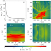 |
Fig. 1 (a) Initial water ion density following a capped version of the profile in Eq. (1) fading out at r = 930 m. (b–d) Final densities (t = 30 ms) in three different planes. |
3 Results
The result confirms that there are three important contributions to the electric field in the inner coma of a comet: the convective solar wind electric field, the ambipolar electric field, and the polarisation electric field. An illustration of the three fields is shown in Fig. 2. This section describes how this comes about, concentrating on the polarisation field in particular.
3.1 Electric field direction
Virtual probes that record the electric field at specific grid points were used in the simulation, and the electric field components recorded by seven of these probes are shown in Fig. 3. Figure 3a shows the field at (x, y, z) = (4, 4, 4) m. Due to the definition of the grid, this is the closest to the origin that the field is known. The other six panels show the electric field components 100 m from the origin in each direction along the coordinate axes. The field recorded by all seven probes first shows some transient oscillations that are followed by the build-up of an electric field with significant positive Ez and negative Ex components. For the probe atz = −100 m (Fig. 3d) this only happens just before the end of the simulation run. Apart from some initial transient oscillations, the Ey component, which is parallel to the magnetic field, is close to zero at all probe locations. The probe positions in the x–z plane are indicated in Fig. 4b.
Figure 4 shows the projection of the electric field in the x–z plane onto that plane for times t = 0.6, 6, 12, 18, 24, and 30 ms. The magnitude  is colour-coded and the direction is shown by arrows in the figure. The right-hand column shows a zoomed-in view of the panels in the left-hand column. Since the plasma is not in an equilibrium state at the beginning of the simulation, some transient oscillations occur. This can be seen both in panels a–c and g–i of Fig. 4 and in Fig. 3, which shows the electric field at the virtual probe positions. In Fig. 4 and the following figures, only the inner region of the simulation (− 500 m ≤|x|, |z|≤ 500 m) is shown in order to avoid presenting artificial effects near the boundary, such as the ramping down of the cometary plasma density to zero described in Sect. 2.
The motion of the solar wind perpendicular to the magnetic field gives rise to a convective electric field Econv = −u0 ×B0. With values from Table 1 it is 0.85 Vm−1 in the positive z direction. Superimposed on this field is an ambipolar field directed opposite to the density gradient, and it can be seen, directed away from the origin, in Figs. 4c–f. The ambipolar field is caused by electrons moving away from the density maximum faster than the ions. This causes an electric field directed radially outward. The total field is stronger on the positive z side of the density maximum because there the convective and ambipolar fields are approximately parallel. On the negative z side they are approximately antiparallel and counteract each other. This affects the ion motion as discussed in Sect. 3.3. The ion motion in turn moves the density maximum, which leads to the stronger field moving toward lower z values with time (Figs. 4b–f). This is also what causes the build-up of the electric field to be observed at different times at the different probe locations.
The third important electric field contribution comes from the polarisation electric field. To a first approximation it can be seen as the response of the cometary plasma to the convective electric field as described by Nilsson et al. (2018). The cometary ions move in the direction of the convective electric field, whereas the electrons E ×B drift perpendicular to it, causing a charge separation that gives rise to the polarisation field in the x–z plane. This field counteracts further charge separation, and thus quasi-neutrality can be maintained (Schottky 1924). The resulting total field has a negative x component, which is seen in Figs. 4j–l. This component is stable even 100 m from the origin, as is shown by the electric field probes (Fig. 3). Comparing panels b and e of Fig. 3, we see that the Ex component is more negative at x = −100 m (where the ambipolar and polarisation fields are both directed in the negative x direction) than at x = 100 m (where the ambipolar field has a positive and the polarisation field a negative x component). The total Ex component is still negative at x = 100 m, which shows that the contribution from the polarisation electric field is stronger than the ambipolar field at that point. The ambipolar electric field also causes an E ×B drift, but since the ambipolar field at the start of the simulation is spherically symmetric, the resulting trajectories are helices, which do not contribute to the net charge that causes the polarisation field. This still holds approximately as the simulation progresses; the spherical symmetry is broken, but the equipotential contours corresponding to the ambipolar field approximately follow contours of equal density, and the electron trajectories form closed loops.
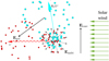 |
Fig. 2 Schematic illustration of the convectional (Econv), ambipolar (Eambi), and polarisation (Epol) contributions to the electric field and illustration of charged particle motion. |
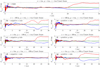 |
Fig. 3 Electric field components as functions of time for seven different grid points where the simulated field is known. (a) (x, y, z) = (4, 4, 4) m, one of the grid points closest to the origin. (b) (x, y, z) = (−100, 4, 4) m, near the negative x-axis. (c) (x, y, z) = (4, − 100, 4) m, near the negative y-axis. (d) (x, y, z) = (4, 4, − 100) m, near the negative z-axis. (e) (x, y, z) = (100, 4, 4) m, near the positive x-axis. (f) (x, y, z) = (4, 100, 4) m, near the positive y-axis. (g) (x, y, z) = (4, 4, 100) m, near the positive z-axis. |
3.2 Density structures
Figures 1b–d show the plasma density in the y–z, x–z, and x–y planes, respectively, at t = 30 ms, which is the end of the simulation run. It can be seen in panels b and d that field aligned structures have formed in the plasma. In all three panels b–d there are structures indicative of waves in the plasma. We do not study these further in this article, and instead focus on quasi-steady-state phenomena. The density maximum is located at negative z values, stretching toward negative x values. This tendency has also been observed in hybrid simulations (Lindkvist et al. 2018), and it is a result of the ion motion described in Sect. 3.3.
3.3 Ion motion
Figure 5 shows the density of the solar wind protons at times t = 0.6, 6, 12, 18, 24, and 30 ms. The velocity of the protons is indicated by arrows in each of the panels. At t = 0.6 ms (Fig. 5a) both density and velocity are close to their initial values. In panel b, at t = 6 ms, the arrows show that the velocity of the protons has acquired a negative vz component. This is consistent with gyration in the magnetic field in the absence of an electric field or in a weak electric field. In the solar wind protons move approximately along straight lines at the velocity E ×B∕B2. Close to the centre of the comet the electric field is weak at t = 6 ms, as shown in Fig. 4b. The gyroradius for a proton moving at 430 km s−1 across a 1.98 μT magnetic field is 2.26 km, which is somewhat larger than the simulated region. This deflection of the protons persists in the next frame (Fig. 5c at t = 12 ms), and later a wake is developed, as is seen in Figs. 5e and f. The formation of a wake is due to electric field deflection of the protons away from the region with high water ion density. The proton density inhomogeneities that change from frame to frame in panels a–c are wave-related transients that arise from the non-equilibrium initialisation of the simulated plasma.
Figure 6 shows the density of cometary H2 O+ ions at times t = 0.6, 6, 12, 18, 24, and 30 ms on a logarithmic colour scale. The ion velocity is indicated by arrows in each panel. In panel a, at t = 0.6 ms, the density follows the capped Eq. (1) profile of the initial plasma. In panel b (t =6 ms) the H2 O+ ions are moving outward due to the ambipolar electric field, and this effect is large enough to cause a density depletion at the origin. This depletion remains in the next panel (Fig. 6c, t = 12 ms). After that the density maximum moves toward negative z values as was seen in Fig. 1. Since the H2 O+ ion density is much higher than the proton density close to the origin, the H2 O+ density in Fig. 6f closely resembles the zoomed-in plot of the plasma density in Fig. 1c.
The reason for the motion of the density maximum toward negative z values is that H2 O+ preferentially leaves the inner coma in the positive z direction, and thereby deplete the plasma on the positive z side of the origin. On the positive z side the convectional and ambipolar electric fields are approximately parallel, and they therefore work together to accelerate water ions away from the central coma. On the negative z side the convectional and ambipolar fields are approximately antiparallel, and they therefore counteract each other, which leads to the removal of cometary plasma being less efficient for negative than positive z coordinates.
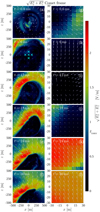 |
Fig. 4 Electric field in the x–z plane for times t = 0.6, 6, 12, 18, 24, and 30 ms. The right column shows a zoomed-in view of the panels in the left column. Each row shows a different instance in time as indicated in each panel. The positions of the probes (cf. Fig. 3) in the x–z plane are indicated in panel b. The sun is to the right, and the magnitude of the convective electric field Econv = 0.85 Vm−1 is indicated on the colour scale. All electric fields are shown in the comet frame of reference. |
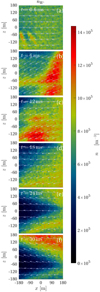 |
Fig. 5 Proton density in the x–z plane for times t = 0.6, 6, 12, 18, 24, and 30 ms. The density is the colour-coded for quantity, and the arrows indicate the proton velocity. Each row shows adifferent instance in time as indicated in each panel. |
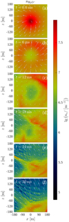 |
Fig. 6 Waterion density in the x–z plane for times t = 0.6, 6, 12, 18, 24, and 30 ms. The colour-coded quantity is the logarithm of the density, and the arrows indicate the water ion velocity. Each row shows a different instance in time, as indicated in each panel. |
3.4 Comparison to observations
An anti-sunward component of the cometary ion velocity was observed several times during the Rosetta mission. Nilsson et al. (2015b) presented histograms of how the water group ion velocities deviate from the radial direction out from the nucleus during Rosetta’s inbound journey between 3.6 and 2.0 AU from the Sun. Behar et al. (2016) examined one day in that period more closely, 28 November 2014 when the heliocentric distance was 2.88 AU. Anti-sunward water group ion velocities were also noticed by Berčič et al. (2018) during the month of January 2015 and by Behar et al. (2018) during Rosetta’s tailward excursion in March and April 2016 at 2.7 AU from the Sun.
The anti-sunward ion velocity components that were observed by Rosetta are consistent with the negative vx components of the H2 O+ ion velocities in the simulations reported here. (Fig. 6). In these simulations the negative vx component is caused by the negative Ex component that arises from the polarisation electric field. Figure 3 shows that this anti-sunward electric field component exists in the simulation at least out to 100 m from the centre of the nucleus. Because of the scaling applied in setting up the simulation (cf. Sect. 2), this corresponds to a cometocentric distance of 40 km at comet 67P. Rosetta was close to the terminator plane at approximately 28 km cometocentric distance during the measurements reported by Berčič et al. (2018). Thus, the simulations produce anti-sunward electric fields over cometocentric distances that are relevant in an observational context. The cometocentric distance was similar for the observations reported by Behar et al. (2016) and for most of the interval studied by Nilsson et al. (2015b). Berčič et al. (2018) observed that the plasma density was higher in the negative z than in the positive z hemisphere in agreement with our results in Sect 3.2. The simulations reported here are consistent with these observations at comet 67P (Nilsson et al. 2015b; Behar et al. 2016; Berčič et al. 2018).
The tailward excursion extended out to 1000 km cometocentric distance which, although it scales down to 2.5 km in our simulation coordinates, is beyond the boundary of the simulation box. The observed ion velocities also showed an anti-sunward component there. However, on the tailward (x < 0) side of the comet, the ambipolar electric field also has an anti-sunward component, and the deviation from a radially directed water ion velocity reported by Behar et al. (2018) was about 10°, which is less than the 22.5° resolution of the instrument. For a detailed comparison of simulations and observations in the tail region we would need a simulation that covers a larger region and a spacecraft equipped with a higher angular resolution ion analyser.
The deflection of the protons toward negative vz values, which occurs during part of the simulated period (see Sect. 3.3), is caused by the total electric field being weaker thanthe convective electric field of the solar wind, and this allows the protons to start gyrating. While this effect could occur at a real comet, there is also another reason for deflection that is not included in our simulations. Near the comet, the magnetic field is piled up and is stronger than the interplanetary magnetic field, and this causes the solar wind protons to be deflected. Since the magnetic field is uniform in our simulation, this is not an effect that we can observe. However, if the magnetic field is approximately uniform over the simulated part of the coma, this deflection could be accounted for by a rotation of the coordinate system. The region over which the magnetic field is uniform can be estimated on average from Rosetta data (see Appendix A). The average field was approximately constant over 60 km ≲ r ≲ 120 km on the first approach in August 2014, and the constant field region extended farther out during the close flybys in February 2015. However, in order to know whether the magnetic field can be seen as uniform at one moment in time and how much it differs from the solar wind magnetic field, simultaneous measurements at multiple points in space are necessary.
4 Conclusions and discussion
We used an electrostatic particle-in-cell simulation to study the electric field at comet 67P/Churyumov-Gerasimenko. There are three major contributions to the electric field: the convectional field of the solar wind, the ambipolar field caused by the high photo-electron thermal speed, and the polarisation electric field that is driven by charged separation due to the vastly different trajectories followed by the electrons and ions. This is illustrated in Fig. 2.
Nilsson et al. (2018) used an analytic model in a cylindrical geometry to show that polarisation of the inner ion coma of a comet causes the electric field to have an anti-sunward component. Our simulation results confirm the existence of such a field, and that it is consistent with observations by the Rosetta spacecraft (Nilsson et al. 2015b; Behar et al. 2016; Berčič et al. 2018). Our simulation starts with a spherically symmetric comet plasma profile, but like Nilsson et al. (2018) we assumed a uniform magnetic field. As the simulation progresses, field-aligned density structures develop (Fig. 1), and the plasma can be approximated by a cylinder, albeit with a non-circular cross section. The use of a uniform magnetic field is reasonable at large heliocentric distances, where despite the magnetic pile-up the magnetic field is approximately constant over a significant part of the coma. We chose to simulate a case where the comet was 3.0 AU from the Sun. When field line draping becomes important, a model with straight field lines may still be valid as long as the simulated region is small compared to the radius of curvature of the draped field. Magnetic field gradients close to the nucleus may still be present, and a model that includes such gradients would then be a better approximation. However, to know what gradients are present, we would need to measure the magnetic field at different positions at the same time, using multiple spacecraft. Nilsson et al. (2018) compared their model to data from the whole period from Rosetta’s arrival at comet 67P to the end of the mission and found it to hold throughout as far as the existence of a polarisation electric field is concerned, although differences between the model and observations exist regarding the precise magnitude and direction of the field. The simulation presented here also includes the ambipolar electric field, making it more realistic. Nevertheless, it also has important limitations.
One obvious limitation is that the simulations are electrostatic, and we therefore cannot follow how the magnetic field develops in time. This means that we are unable to realistically reproduce a bow shock, which at a real comet exhibits a significant magnetic field gradient. For a weak comet far from the Sun, such as the one simulated here, bow shocks are less likely to occur, and the magnetic field is less influenced by field line draping than closer to perihelion. At 3.0 AU heliocentric distance, the simulation presented confirms the existence of a polarisation electric field, even though it does not reproduce the complete magnetic field behaviour of the cometary plasma. Nilsson et al. (2018) found that a polarisation field existed throughout Rosetta’s journey alongside comet 67P. This includes the period when a bow shock had formed upstream of the nucleus. Potentially this simulation model could also be used for that time period, if only the region close to the nucleus and completely downstream of the shock were considered and a shocked solar wind plasma was injected at the upstream boundary. Still, the times around perihelion when a diamagnetic cavity has formed are out of reach for electrostatic models and require electromagnetic simulation codes.
In this simulation the whole density structure is allowed to move since, unlike the plasma at a real comet, it is not anchored to a solid nucleus and plasma production is not included in the model after the initialisation of a fixed profile at the start. However, at a real comet the convective and ambipolar fields also affect the plasma, as they do in the simulation, and this will result in a similar asymmetry. Furthermore, the extent of the density structure is a few hundred metres in this simulation (Fig. 1c), whereas the nucleus radius scales down to only 5 m in the simulated system. Thus, the density structure affected by the electric field is much larger than the nucleus. If simultaneous measurements could be made at different locations around a comet, we would expect a density structure that is similar to what we have simulated, to be observed with a local perturbation near the nucleus that is not accounted for here.
Previous hybrid simulations of comets, which treat ions as particles and the electrons as a fluid, have mostly focused on heliocentric distances close to perihelion when the outgassing rates are high (Koenders et al. 2013, 2015; Simon Wedlund et al. 2017). Those simulations are not directly comparable to ours. Lindkvist et al. (2018) have performed hybrid simulations of a comet at intermediate outgassing rates and Deca et al. (2017) model a weakly outgassing comet, using an implicit particle-in-cell method, which does not resolve electron scales, and therefore can be seen as equivalent to a hybrid simulation. Both of these methods aim to model larger spatial scales than we do. However, some similarities may be seen. The simulations by Deca et al. (2017) and Lindkvist et al. (2018), and our simulation as well, show a cometary ion density structure extending in the direction opposite to the cometary ion bulk velocity direction. The protons form a wake behind the comet in our case and in that of Deca et al. (2017). The simulations by Lindkvist et al. (2018) also show a proton wake, but due to the higher activity other phenomena, like shock formation, also appear in that simulation and a direct comparison cannot readily be performed.
We confirmed the existence of a polarisation electric field in the inner coma of a comet, using an electrostatic particle-in-cell simulation that also models the ambipolar electric field in that region. Both these fields contribute significantly to the total electric field and are an important influence on ion motion in the head of a comet, demonstrating the necessity to include space charge effects in a description of cometary plasma. The results are consistent with previously published observations of both cometary ion motion and the plasma density distribution around the comet.
The intention of this paper has been to present a qualitative study of the electric fields at a comet. A quantitative comparison must be seen as the next step to be taken in a future study, as a simulation that develops in time is not readily comparable to stationary analytical models. In order to obtain useful quantitative estimates we would need to update our present model to also account for plasma production by ionisation of the cometary neutrals. In this paper we simulated only 30 ms, that is to say a timescale on which ionisation does not change the results. To reach an equilibrium between plasma production and plasma transport it is necessary to simulate a few seconds even for our scaled-down comet. This corresponds to approximately 100 times the duration of our present simulation run, and it would not be practical as it would require continuous running of the simulation program for about two years. However, including ionisation during the simulation and running it for a somewhat longer time, although not to equilibrium, can be done, and then the importance of continuous ionisation in the modelling of comets can be assessed. The inclusion of ionisation will also enable a comparison to both analytical models (e.g. Beth & Galand 2018) and measurements of ion speeds (Odelstad et al. 2018) and densities (Edberg et al. 2015) with the aim of understanding how plasma is produced and transported in the coma. If the thus described update is combined with a routine for following a statistically significant number of particle trajectories in the simulation, it would also be possible to tell how the plasma moves around the comet and how particles contribute to observed velocities and densities. Finally, the role of wave particle interaction is a topic that deserves consideration in future work. Electrostatic simulations, like the one reported here, can be used to model ion acoustic-like waves in plasmas. As we note in Sect. 3.2, wave signatures can be seen in the plasma, and even the motion of large-scale field and density structures can be described in terms of waves. Electrostatic simulations may be employed to assess the role of waves in the inner coma and to what extent waves can modify the steady-state picture of plasma transport.
Acknowledgements
The software used in this work was developed by J.L. and H.G. and is available for download at https://doi.org/10.5281/zenodo.2656629. This research was conducted using the resources of High Performance Computing Center North (HPC2N) at Umeå University. This work was supported by the Swedish National Space Agency (grants 201/15 and 108/18). Work at the Belgian Institute for Space Aeronomy was supported by the Belgian Science Policy Office through the Solar-Terrestrial Centre of Excellence.
Appendix A Magnetic field profile
In order to evaluate the uniformity of the magnetic field we used magnetic field data from the RPC-MAG instrument (Glassmeier et al. 2007b) on board the Rosetta spacecraft. Figure A.1 shows the magnetic field during two three-week periods: 3–24 August 2014, during the first approach of Rosetta to comet 67P, when the comet was at 3.6 AU heliocentric distance (Figs. A.1a–b) and between 31 January and 21 February 2015 at approximately 2.4 AU (Figs. A.1c–d). These periods were chosen because they are the only times during the mission with a fast cometocentric distance variation and good coverage of distances.
The upper panels (Figs. A.1a and c) show the magnitude of the magnetic flux density as a function of time, down-sampled to a sampling period of 5 s. The temporal variations are seen to be large. In the lower panels (Figs. A.1b and d) the data have been sorted according to cometocentric distance. The black curves show a 4000 point running median of the sorted data.
There are large temporal fluctuations, but the median field stays relatively constant around 4 nT from r ≈ 60 km to r ≈ 120 km during the first approach (Fig. A.1b). Outside r ≈ 120 km there is a systematic decrease in the magnetic field with increasing cometocentric distance. The peak at r ≈ 300 km is a result of theevent that lead to the magnetic field peaking on 3 August. During the three-week period in February 2015 shown in panels c and d, the temporal variations were larger than during first approach. The median field stayed in the 10–20 nT range out to r≈ 250 km. Large-scale fluctuations are typical of the plasma at comet 67P (Goetz et al. 2017).
The data shown in Fig. A.1 supports the existence of a spatial gradient in the magnitude of the magnetic field between approximately 120 and 200 km cometocentric distance during Rosetta’s first approach to the comet in August 2014. Closer to the comet during that time and over the whole range of cometocentric distances probed during February 2015, the data does not indicate the presence of spatial gradients. The magnetic field fluctuations observed there are more likely to result from temporal variations driven by the solar wind. However, since these observations were performed by a single spacecraft, the presence of spatial gradients can only be ruled out on average. To completely determine whether spatial gradients exist at a particular moment in time requires simultaneous measurements at multiple points in space.
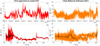 |
Fig. A.1 Magnetic flux density measurements by the RPC-MAG instrument on board the Rosetta spacecraft during two different three-week periods. (a) |B| as a function of time during the first approach to comet 67P as a function of time. (b) The data in panel a reordered according to cometocentric distance. (c) |B| as a function of time during the close flybys in February 2015. (d) The data in panel c reordered according to cometocentric distance. The black curves show a running median of the sorted data. |
References
- Behar, E., Nilsson, H., Stenberg Wieser, G., et al. 2016, Geophys. Res. Lett., 43, 1411 [NASA ADS] [CrossRef] [Google Scholar]
- Behar, E., Nilsson, H., Henri, P., et al. 2018, A&A, 616, A21 [NASA ADS] [CrossRef] [EDP Sciences] [Google Scholar]
- Berčič, L., Behar, E., Nilsson, H., et al. 2018, A&A, 613, A57 [NASA ADS] [CrossRef] [EDP Sciences] [Google Scholar]
- Beth, A., & Galand, M. 2018, MNRAS, 469, S824 [CrossRef] [Google Scholar]
- Birdsall, C. K., & Langdon, A. B. 1991, Plasma Physics via Computer simulation (Bristol, UK: IOP Publishing Ltd.) [CrossRef] [Google Scholar]
- Brenning, N., Kelley, M. C., Providakes, J., Swenson, C., & Stenbaek-Nielsen, H. C. 1991, J. Geophys. Res., 96, 9735 [NASA ADS] [CrossRef] [Google Scholar]
- Brenning, N., Hurtig, T., & Raadu, M. A. 2005, Phys. Plasmas, 12, 012309 [NASA ADS] [CrossRef] [Google Scholar]
- Coates, A. J., & Jones, G. H. 2009, Planet. Space Sci., 57, 1175 [NASA ADS] [CrossRef] [Google Scholar]
- Deca, J., Divin, A., Henri, P., et al. 2017, Phys. Rev. Lett., 118, 205101 [NASA ADS] [CrossRef] [Google Scholar]
- Edberg, N. J. T., Eriksson, A. I., Odelstad, E., et al. 2015, Geophys. Res. Lett., 42, 4263 [NASA ADS] [CrossRef] [Google Scholar]
- Eriksson, A. I., Engelhardt, I. A. D., André, M., et al. 2017, A&A, 605, A15 [NASA ADS] [EDP Sciences] [Google Scholar]
- Galand, M., Héritier, K. L., Odelstad, E., et al. 2016, MNRAS, 462, S331 [CrossRef] [Google Scholar]
- Glassmeier, K.-H., Boehnhardt, H., Koschny, D., Kührt, E., & Richter, I. 2007a, Space Sci. Rev., 128, 1 [NASA ADS] [CrossRef] [Google Scholar]
- Glassmeier, K.-H., Richter, I., Diedrich, A., et al. 2007b, Space Sci. Rev., 128, 649 [NASA ADS] [CrossRef] [Google Scholar]
- Goetz, C., Koenders, C., Richter, I., et al. 2016a, A&A, 588, A24 [Google Scholar]
- Goetz, C., Koenders, C., Hansen, K. C., et al. 2016b, MNRAS, 462, S459 [Google Scholar]
- Goetz, C., Volwerk, M., Richter, I., & Glassmeier, K.-H. 2017, MNRAS, 469, S268 [CrossRef] [Google Scholar]
- Gunell, H., Hurtig, T., Nilsson, H., Koepke, M., & Brenning, N. 2008, Plasma Phys. Control. Fusion, 50, 074013 [NASA ADS] [CrossRef] [Google Scholar]
- Gunell, H., Walker, J. J., Koepke, M. E., et al. 2009, Phys. Plasmas, 16, 112901 [NASA ADS] [CrossRef] [Google Scholar]
- Gunell, H., Nilsson, H., Stenberg, G., et al. 2012, Phys. Plasmas, 19, 072906 [NASA ADS] [CrossRef] [Google Scholar]
- Gunell, H., Mann, I., Simon Wedlund, C., et al. 2015, Planet. Space Sci., 119, 13 [NASA ADS] [CrossRef] [Google Scholar]
- Gunell, H., Goetz, C., Eriksson, A., et al. 2017, MNRAS, 469, S84 [CrossRef] [Google Scholar]
- Gunell, H., Goetz, C., Simon Wedlund, C., et al. 2018, A&A, 619, L2 [NASA ADS] [CrossRef] [EDP Sciences] [Google Scholar]
- Hansen, K. C., Altwegg, K., Berthelier, J.-J., et al. 2016, MNRAS, 462, S491 [Google Scholar]
- Herlofson, N. 1951, Arkiv för fysik, 3, 247 [Google Scholar]
- Hockney, R. W., & Eastwood, J. W. 1988, Computer Simulation Using Particles (Bristol, UK: IOP Publishing Ltd.) [CrossRef] [Google Scholar]
- Huebner, W. F., & Mukherjee, J. 2015, Planet. Space Sci., 106, 11 [Google Scholar]
- Hurtig, T. 2004, PhD Thesis, Royal Institute of Technology (KTH), Stockholm, Sweden [Google Scholar]
- Hurtig, T., Brenning, N., & Raadu, M. A. 2003, Phys. Plasmas, 10, 4291 [NASA ADS] [CrossRef] [Google Scholar]
- Hurtig, T., Brenning, N., & Raadu, M. A. 2004, Phys. Plasmas, 11, L33 [CrossRef] [Google Scholar]
- Johnstone, A. D., Coates, A. J., Huddleston, D. E., et al. 1993, A&A, 273, L1 [NASA ADS] [Google Scholar]
- Kallio, E., & Jarvinen, R. 2012, Earth Planets Space, 64, 157 [NASA ADS] [CrossRef] [Google Scholar]
- Karlsson, T., Eriksson, A. I., Odelstad, E., et al. 2017, Geophys. Res. Lett., 44, 1641 [NASA ADS] [Google Scholar]
- Koenders, C., Glassmeier, K.-H., Richter, I., Motschmann, U., & Rubin, M. 2013, Planet. Space Sci., 87, 85 [NASA ADS] [CrossRef] [Google Scholar]
- Koenders, C., Glassmeier, K.-H., Richter, I., Ranocha, H., & Motschmann, U. 2015, Planet. Space Sci., 105, 101 [NASA ADS] [CrossRef] [Google Scholar]
- Lindkvist, J., & Gunell, H. 2019, Picard – an electrostatic particle in cell simulation code https://doi.org/10.5281/zenodo.2656629 [Google Scholar]
- Lindkvist, J., Holmström, M., Fatemi, S., Wieser, M., & Barabash, S. 2017, Geophys. Res. Lett., 44, 2070 [NASA ADS] [Google Scholar]
- Lindkvist, J., Hamrin, M., Gunell, H., et al. 2018, A&A, 616, A81 [NASA ADS] [CrossRef] [EDP Sciences] [Google Scholar]
- Madsen, B., Simon Wedlund, C., Eriksson, A., et al. 2018, Geophys. Res. Lett., 45, 3854 [NASA ADS] [CrossRef] [Google Scholar]
- Mandt, K. E., Eriksson, A., Edberg, N. J. T., et al. 2016, MNRAS, 462, S9 [Google Scholar]
- Meier, P., Glassmeier, K.-H., & Motschmann, U. 2016, Ann. Geophys., 34, 691 [NASA ADS] [CrossRef] [Google Scholar]
- Nilsson, H., Stenberg Wieser, G., Behar, E., et al. 2015a, Science, 347, aaa0571 [NASA ADS] [CrossRef] [Google Scholar]
- Nilsson, H., Stenberg Wieser, G., Behar, E., et al. 2015b, A&A, 583, A20 [NASA ADS] [CrossRef] [EDP Sciences] [Google Scholar]
- Nilsson, H., Stenberg Wieser, G., Behar, E., et al. 2017, MNRAS, 469, S252 [Google Scholar]
- Nilsson, H., Gunell, H., Karlsson, T., et al. 2018, A&A, 616, A50 [NASA ADS] [CrossRef] [EDP Sciences] [Google Scholar]
- Odelstad, E., Eriksson, A. I., Edberg, N. J. T., et al. 2015, Geophys. Res. Lett., 42, 10126 [NASA ADS] [CrossRef] [EDP Sciences] [Google Scholar]
- Odelstad, E., Eriksson, A. I., Johansson, F. L., et al. 2018, J. Geophys. Res. Space Phys., 123, 5870 [NASA ADS] [CrossRef] [Google Scholar]
- Plaschke, F., Hietala, H., Archer, M., et al. 2018, Space Sci. Rev., 214, 81 [NASA ADS] [CrossRef] [Google Scholar]
- Richter, I., Koenders, C., Auster, H.-U., et al. 2015, Ann. Geophys., 1031 [Google Scholar]
- Richter, I., Auster, H.-U., Berghofer, G., et al. 2016, Ann. Geophys., 34, 609 [NASA ADS] [CrossRef] [Google Scholar]
- Schottky, W. 1924, Phys. Z., 25, 342 [Google Scholar]
- Simon Wedlund, C., Alho, M., Gronoff, G., et al. 2017, A&A, 604, A73 [NASA ADS] [CrossRef] [EDP Sciences] [Google Scholar]
- Tonks, L. 1931, Phys. Rev., 37, 1458 [NASA ADS] [CrossRef] [Google Scholar]
- Vigren, E., & Eriksson, A. I. 2017, AJ, 153, 150 [NASA ADS] [CrossRef] [Google Scholar]
- Vigren, E., André, M., Edberg, N. J. T., et al. 2017, MNRAS, 469, S142 [Google Scholar]
- Voitcu, G., & Echim, M. 2016, J. Geophys. Res. Space Phys., 121, 4343 [NASA ADS] [CrossRef] [Google Scholar]
- Voitcu, G., & Echim, M. 2017, Geophys. Res. Lett., 44, 5920 [NASA ADS] [CrossRef] [Google Scholar]
- Voitcu, G., & Echim, M. 2018, Ann. Geophys., 36, 1521 [NASA ADS] [CrossRef] [Google Scholar]
All Tables
Solar wind and cometary conditions and respective cometary and simulation values.
All Figures
|
Fig. 1 (a) Initial water ion density following a capped version of the profile in Eq. (1) fading out at r = 930 m. (b–d) Final densities (t = 30 ms) in three different planes. |
| In the text | |
|
Fig. 2 Schematic illustration of the convectional (Econv), ambipolar (Eambi), and polarisation (Epol) contributions to the electric field and illustration of charged particle motion. |
| In the text | |
|
Fig. 3 Electric field components as functions of time for seven different grid points where the simulated field is known. (a) (x, y, z) = (4, 4, 4) m, one of the grid points closest to the origin. (b) (x, y, z) = (−100, 4, 4) m, near the negative x-axis. (c) (x, y, z) = (4, − 100, 4) m, near the negative y-axis. (d) (x, y, z) = (4, 4, − 100) m, near the negative z-axis. (e) (x, y, z) = (100, 4, 4) m, near the positive x-axis. (f) (x, y, z) = (4, 100, 4) m, near the positive y-axis. (g) (x, y, z) = (4, 4, 100) m, near the positive z-axis. |
| In the text | |
|
Fig. 4 Electric field in the x–z plane for times t = 0.6, 6, 12, 18, 24, and 30 ms. The right column shows a zoomed-in view of the panels in the left column. Each row shows a different instance in time as indicated in each panel. The positions of the probes (cf. Fig. 3) in the x–z plane are indicated in panel b. The sun is to the right, and the magnitude of the convective electric field Econv = 0.85 Vm−1 is indicated on the colour scale. All electric fields are shown in the comet frame of reference. |
| In the text | |
|
Fig. 5 Proton density in the x–z plane for times t = 0.6, 6, 12, 18, 24, and 30 ms. The density is the colour-coded for quantity, and the arrows indicate the proton velocity. Each row shows adifferent instance in time as indicated in each panel. |
| In the text | |
|
Fig. 6 Waterion density in the x–z plane for times t = 0.6, 6, 12, 18, 24, and 30 ms. The colour-coded quantity is the logarithm of the density, and the arrows indicate the water ion velocity. Each row shows a different instance in time, as indicated in each panel. |
| In the text | |
|
Fig. A.1 Magnetic flux density measurements by the RPC-MAG instrument on board the Rosetta spacecraft during two different three-week periods. (a) |B| as a function of time during the first approach to comet 67P as a function of time. (b) The data in panel a reordered according to cometocentric distance. (c) |B| as a function of time during the close flybys in February 2015. (d) The data in panel c reordered according to cometocentric distance. The black curves show a running median of the sorted data. |
| In the text | |
Current usage metrics show cumulative count of Article Views (full-text article views including HTML views, PDF and ePub downloads, according to the available data) and Abstracts Views on Vision4Press platform.
Data correspond to usage on the plateform after 2015. The current usage metrics is available 48-96 hours after online publication and is updated daily on week days.
Initial download of the metrics may take a while.