| Issue |
A&A
Volume 682, February 2024
|
|
|---|---|---|
| Article Number | A62 | |
| Number of page(s) | 10 | |
| Section | Planets and planetary systems | |
| DOI | https://doi.org/10.1051/0004-6361/202348186 | |
| Published online | 05 February 2024 | |
Impact of radial interplanetary magnetic fields on the inner coma of comet 67P/Churyumov-Gerasimenko
Hybrid simulations of the plasma environment
1
Department of Physics, Umeå University,
901 87
Umeå,
Sweden
e-mail: This email address is being protected from spambots. You need JavaScript enabled to view it.
2
Department of Mathematics, Physics and Electrical Engineering, Northumbria University,
Newcastle-upon-Tyne,
UK
Received:
6
October
2023
Accepted:
25
November
2023
Abstract
Context. The direction of the interplanetary magnetic field determines the nature of the interaction between a Solar System object and the solar wind. For comets, it affects the formation of both a bow shock and other plasma boundaries, as well as mass-loading. Around the nucleus of a comet, there is a diamagnetic cavity, where the magnetic field is negligible. Observations by the Rosetta spacecraft have shown that, most of the time, the diamagnetic cavity is located within a solar-wind ion cavity, which is devoid of solar wind ions. However, solar wind ions have been observed inside the diamagnetic cavity on several occasions. Understanding what determines whether or not the solar wind can reach the diamagnetic cavity also advances our understanding of comet–solar wind interaction in general.
Aims. We aim to determine the influence of an interplanetary magnetic field directed radially out from the Sun – that is, parallel to the solar wind velocity – on the comet–solar wind interaction. In particular, we explore the possibility of solar wind protons entering the diamagnetic cavity under radial field conditions.
Methods. We performed global hybrid simulations of comet 67P/Churyumov-Gerasimenko using the simulation code Amitis for two different interplanetary magnetic field configurations and compared the results to observations made by the Rosetta spacecraft.
Results. We find that, when the magnetic field is parallel to the solar wind velocity, no bow shock forms and the solar wind ions are able to enter the diamagnetic cavity. A solar wind ion wake still forms further downstream in this case.
Conclusions. The solar wind can enter the diamagnetic cavity if the interplanetary magnetic field is directed radially from the Sun, and this is in agreement with observations made by instruments on board the Rosetta spacecraft.
Key words: plasmas / methods: numerical / comets: general / comets: individual: 67P/Churyumov-Gerasimenko
Note to the reader: Figure 6 was not displayed correctly. The image was rectified on 20 February 2024.
© The Authors 2024
 Open Access article, published by EDP Sciences, under the terms of the Creative Commons Attribution License (https://creativecommons.org/licenses/by/4.0), which permits unrestricted use, distribution, and reproduction in any medium, provided the original work is properly cited.
This article is published in open access under the Subscribe to Open model. This email address is being protected from spambots. You need JavaScript enabled to view it. to support open access publication.
1 Introduction
The outgassing of comets and subsequent ionisation of the neutral gas leads to the formation of a plasma cloud around the nucleus. The neutral gas cloud is mostly made up of water and expands slowly (1 km s−1), and the ions start out at that speed after ionisation, but are subsequently accelerated to higher speeds because of the presence of electric fields. The cometary plasma also contains an electron population that ensures quasineutrality. As the comet traverses the Solar System, the outgassing rate changes, and therefore so does the plasma density. This changing plasma cloud is encountered by the solar wind and presents an obstacle to the plasma flow (see Goetz et al. 2022a, for a review of plasma physics at comets). The cometary (heavy) ions add free energy to the flowing solar wind, which is released as the ions are incorporated into the solar wind flow. When the interplanetary magnetic field (IMF) has a component perpendicular to the solar wind flow direction, mass-loading can be accomplished by pickup of the cometary ions as they E × B drift due to the convective electric field of the solar wind flow. Initially, a newborn cometary ion moves in the direction of the electric field, and, on longer time scales, it follows a cycloid trajectory in the same direction as the solar wind flow. For comet 67P/Churyumov-Gerasimenko (henceforth comet 67P), this was confirmed in observations by the Rosetta spacecraft, and it was also found that the direction of the cometary ion motion near the nucleus of the comet is modified by the presence of an antisunward-polarisation electric field (Behar et al. 2016).
Mass-loading can also be accomplished through waveparticle interactions (e.g. Huddleston & Johnstone 1992). This becomes important when the IMF is directed radially out from – or equivalently in towards – the Sun, and is therefore parallel to the solar wind velocity, as in this case there is no convective electric field. Understanding these processes is fundamental to understanding the plasma environment of a comet, and therefore many attempts have been made to describe them (Tsurutani & Oya 1989; Johnstone 1991). For example, Huddleston & Johnstone (1992) calculated the free energy contained in the cometary ions observed at comet 1P/Halley and found that it depends on the direction of the solar wind magnetic field, being highest when the solar wind velocity is parallel to the magnetic field. The total free energy content is then found to be larger than the magnetic wave energy as it is not released instantaneously. Instead, the energy is slowly released through wave-particle interactions. While acceleration of cometary ions due to the E × B drift has been detected near the location where the ions were born (Nilsson et al. 2015), mass-loading via wave-particle interaction requires larger scales for the ion distribution function to evolve into a shell in velocity space (Scarf et al. 1986). With the lack of convective E-field acceleration, the cometary ions appear as a beam in the velocity space of the solar wind. Such a beam configuration is known to be unstable and has been shown to generate ion cyclotron waves (Glassmeier et al. 1989). Waveparticle interactions have also been invoked as a mechanism to accelerate the heavy ions at comets (Tsurutani & Smith 1986a, b).
The Rosetta spacecraft (Glassmeier et al. 2007) accompanied comet 67P for two years from 2014 to 2016. The first plasma boundary to be observed as the comet approached the Sun was the infant bow shock (IBS; Gunell et al. 2018). The first IBS observation took place on 27 November 2014 at a heliocentric distance of 2.9 AU (Goetz et al. 2021). After the comet reached a heliocentric distance of 1.76 AU, the spacecraft entered the solar wind ion cavity (Behar et al. 2017), which was inaccessible to solar wind ions at that time. At about the same time, the diamagnetic cavity was first observed (Goetz et al. 2016a), which suggested that whenever a diamagnetic cavity exists at a comet, there is also both a solar wind ion cavity surrounding the diamagnetic cavity and a bow shock further upstream. However, on a few occasions, unshocked solar wind protons were observed by the Rosetta spacecraft when it was in the diamagnetic cavity. This means that there are conditions under which a diamagnetic cavity can exist without the presence of either a bow shock or a solar-wind ion cavity. On each of the occasions reported by Goetz et al. (2023), solar wind ions were seen both inside and outside of the diamagnetic cavity.
Goetz et al. (2023) studied five cases in which solar wind protons were found in the innermost coma of comet 67P. The detected protons were of solar wind origin, almost at solar wind speed, and were undeflected. This contradicts expectations given proton observations in the inner coma1, where, at high gas production rates, protons should not be observable at all as the solar-wind ion cavity has formed, or, at intermediate gas production rates, solar wind protons should be deflected due to mass-loading (Behar et al. 2017; Simon Wedlund et al. 2019a). Internal and external transients, such as outbursts, corotating interaction regions, and interplanetary coronal mass ejections were ruled out as factors driving this unusual observation. Charge exchange was also ruled out. The remaining hypothesis is that a radial interplanetary field caused these observations. For a radial field, the convective electric field is zero and therefore cometary ions are not picked up efficiently. This fits the observations, as accelerated pick-up cometary ions are not observable while protons are found in and near the diamagnetic cavity. In return, protons in the solar wind are not deflected and are not slowed, as they retain most of their energy and momentum. This allows solar wind protons to enter the diamagnetic cavity without the distributions being significantly modified. In turn, the lack of pile-up of magnetic field along the streamline creates a lower magnetic pressure outside of the diamagnetic cavity, allowing it to expand (Gombosi et al. 1994). While this hypothesis fits the observation, without a solar wind monitor it cannot be proven definitely.
The case of radial IMF has also been observed at Mars, where the lack of a global magnetic field makes its interaction with the solar wind comparable to that of a comet. Some of the main features observed in the comet case are also observed at Mars (Fowler et al. 2022): (1) protons of solar wind origin are detected within the ionosphere with close to solar wind energies and (2) the location of the magnetic pile up boundary is shifted from above the ionosphere to within the ionosphere where collisions dominate. This indicates inefficient deceleration of the plasma carrying the magnetic field. The presence of a high-energy tail on the planetary ion distribution and significant magnetic field wave activity indicate that wave particle interaction contributes to the energisation of ions in the absence of a convective electric field. At Venus, Chang et al. (2020) analysed 13 radial IMF events observed by the Venus Express spacecraft. These authors found that a radial IMF can demagnetise the ionosphere and also make the magnetic barrier weak and narrow.
Simulations of comet 67P have been performed for heliocentric distances corresponding to different phases of the Rosetta mission. Heliocentric distances of around 3 AU – corresponding to the situation soon after Rosetta’s arrival at the comet - were modelled using both electromagnetic implicit particle-incell simulations (Deca et al. 2019; Divin et al. 2020) and an explicit electrostatic model (Gunell et al. 2019; Gunell & Goetz 2023). The results of the two methods are in overall agreement with each other and show the importance of space charge and Hall effects in the low-activity phase of the comet.
As comet 67P moved closer to the Sun, a bow shock started to form. The initial bow shock formation was modelled using a hybrid simulation technique (Lindkvist et al. 2018), and when observed by Rosetta it was named the infant bow shock (Gunell et al. 2018; Goetz et al. 2021). Further hybrid simulations showed that the stand-off distance of a fully developed bow shock increases as the simulation is made more realistic by including more ionisation processes: photo-ionisation, electron impact ionisation, and charge-exchange processes (Simon Wedlund et al. 2017). The ion energy spectrum and its relationship to the bow shock stand-off distance was simulated by Alho et al. (2019), showing that information regarding the stand-off distance can be obtained by observations of the ion energy spectrogram, as previously suggested by Nilsson et al. (2018).
Koenders et al. (2013) explored the bow shock position in hybrid simulations. These authors studied the reaction of the bow shock position to the variation of different parameters such as magnetic field, outgassing rate, solar wind velocity and density, and, crucially for this study, the Parker angle. Parker angles from 45° to 90° degrees are simulated. The stand-off distance of the bow shock is a measure of the pick-up ‘efficiency’, as the bow shock is a result of the mass-loading of the solar wind flow. The bow shock develops when a critical mass density has been reached and no more mass can be added. Only the transition to a submagnetosonic flow allows additional mass-loading (Biermann et al. 1967). Koenders et al. (2013) found that, as the Parker angle decreases, so does the stand-off distance of the bow shock. This is in line with expectations, as the pick-up associated with the convective electric field is most efficient when the field is largest, which is the case for a magnetic field perpendicular to the solar wind velocity. However, these authors also found that the bow shock distance does not decrease in proportion to the decrease in convective electric field, but instead decreases slowly as the angle decreases. The authors attribute this to additional pick-up due to instabilities and wave-particle interactions.
Koenders et al. (2015) performed hybrid simulations of the cometary environment at a gas production rate of 5 × 1027 s−1 and with a Parker angle of 52°. As expected for those conditions, the solar wind ions are not able to reach the inner coma and a diamagnetic cavity of roughly 30km in radius forms around the nucleus. The simulations also show a filamentation of the plasma density at the diamagnetic cavity boundary, which indicates that the boundary is unstable. The filamentation is not reflected in the magnetic field because numerical diffusion smoothes out any structures of that size.
In this paper, we present hybrid simulations of comet 67P under conditions similar to those found during the observations of solar wind protons in the diamagnetic cavity by Goetz et al. (2023). We address the question of whether or not a parallel magnetic field could be behind those proton observations, and we explore the difference between cometary magnetospheres at parallel and perpendicular IMF using two different IMF directions.
2 Numerical model
The simulations were run using the quasineutral hybrid code Amitis (Fatemi et al. 2017, 2022), which runs on multiple graphics processing units (GPUs). The ions are treated as macroparticles and the electrons as a massless charge-neutralising fluid. The motion of the ions is computed by integration of the Lorentz force. The magnetic field is propagated via Faraday’s law, ∂B/∂t = −∇ × E, where B is the magnetic flux density and E the electric field, which is computed as
 (1)
(1)
where u is the bulk velocity of the ions, J the current density, ρi the charge density of the ions, pe the electron pressure, and η the resistivity. The first term on the right hand side of Eq. (1) is the convective, the second the Hall, the third the ambipolar electric field, and the fourth is a resistive term. The current density is obtained from Ampere’s law with displacement current omitted:
 (2)
(2)
The system of equations is closed by an equation of state assuming adiabatic electrons so that
 (3)
(3)
with the adiabatic index γ = 5/3.
The resistive term is necessary to suppress numerical instabilities, which would otherwise cause artificial waves and fluctuations to appear. On the other hand, the introduction of the resistivity smooths out sharp magnetic field gradients that appear naturally in the plasma. The choice of the value for the resistivity is by necessity a compromise between the requirements to avoid these two effects. In the simulations presented here, we have set η = 2 × 10⁴ Ω m in a sphere of radius 300 km centred at the origin and η = 2 × 10³ Ω m everywhere else. This choice was guided by a series of experimental runs that showed that lower η values than these would cause numerical instabilities in the respective regions.
All quantities are defined on a uniform grid with a grid cell size of ∆x = 50 km. The orthogonal right-handed system is defined so that the solar wind ions are injected at the upper x boundary and the solar wind velocity is in the negative x direction. The coordinate system is oriented so that the convective electric field of the undisturbed solar wind is in the z direction. The simulation domain is defined by −2.0 × 10³ km ≤ x ≤ 2.0 × 10⁴ km, −1.1 × 10⁴ km ≤ y ≤ 1.1 × 10⁴ km, and −1.6 × 10⁴ km ≤ z ≤ 1.0 × 10⁴ km. As in most hybrid and particle-in-cell simulations of comets, the nucleus of the comet is not modelled in the simulation (e.g. Koenders et al. 2016; Deca et al. 2017; Lindkvist et al. 2018; Gunell & Goetz 2023). Instead, the cometary H2O+ ion production rate is computed for each grid cell and the corresponding number of macro-particles are introduced at each time step. The ion production is modelled as ionisation of the neutral coma, the density of which is assumed to follow a Haser model (Haser 1957). We neglect the exponential factor of the Haser model, because it does not have an appreciable influence on the neutral density at cometocentric distances relevant to the Rosetta mission. Thus, the cometary ion production rate per unit volume is
 (4)
(4)
where Qn is the neutral gas production rate, vi the ionisation frequency, ur the radial velocity component of the neutrals, and r the cometocentric distance. The parameters values are listed in Table 1.
The radial velocity ur of the neutrals also becomes the initial velocity of the newborn cometary ions. When the IMF is perpendicular to the solar wind velocity, the cometary ions will be picked up by the solar wind, and their gyroradii will be approximately the same size as the simulation box. This means that they will leave the system while on the first arch of their cycloid orbits. However, as their initial speed is much lower than the solar wind speed, none of these ions would have gyrated back into the simulated region, and therefore this does not affect the results in the region we simulate. What happens to the cometary ion population as they continue further downstream along the ion tail is not included in our model.
Two solar-wind ion species have been included in the simulations: protons (96% of the solar wind ion number density) and alpha particles (4%). The initial transients have subsided after a simulation time of approximately 1 min. At that time, all features on the scale of what is shown in the figures have developed, and the system has entered a quasi-steady state. We refer to this state as quasi-steady, because fluctuations and waves on smaller scales are always present and are part of the physics of the comet. The simulation was run for 192 000 time steps, corresponding to a time of t = 76.8 s, meaning that the comet had entered its quasisteady state. The quantities presented in Sect. 3 are taken at that t = 76.8 s, except the distribution functions; in order to obtain better particle statistics, these latter are an average of the distributions at t = 76.8 s and t = 80 s. The simulation was run for an additional 8000 time steps for this purpose.
Parameters of the simulations.
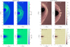 |
Fig. 1 Magnetic flux density and proton density in the x–z and x–y planes at t = 76.8 s for cone angles α = 0° and 90°. (a) |B| in the x–z plane for α = 90°, (b) |B| in the x–y plane for α = 90°, (c) np in the x–z plane for α = 90°, (d) np in the x–y plane for α = 90°, (e) |B| in the x–z plane for α = 0°, (f) |B| in the x–y plane for α = 0°, (g) np in the x–z plane for α = 0°, and (h) np in the x–y plane for α = 0°. The cross symbol (×) marks the position of the nucleus. In the magnetic field panels, the arrows show the direction of the component of B in the plane shown. In the proton density panels, the arrows show the direction of the proton bulk velocity component in the plane shown. |
3 Results
We conducted two simulation runs of the Amitis code with two different cone angles. For the cone angle α = 0°, the IMF is in the − x direction and is therefore parallel to the solar wind velocity. For cone angle α = 90° , the IMF is in the +y direction and therefore the IMF and the solar wind velocity are perpendicular. All other parameters are the same in the two runs, are chosen to model the Rosetta observations by Goetz et al. (2023), and are shown in Table 1. Rosetta observed protons inside the diamagnetic cavity on five occasions from late December 2015 to mid-February 2016. Three of these events occurred on 31 January 2016 when the comet was outbound at a heliocentric distance of 2.25 AU, which is why we have chosen conditions for the simulations that are similar to those found on that date.
3.1 Morphology of the magnetic field and densities
3.1.1 Perpendicular B
Figure 1 shows the magnetic field (|B|) and the proton density (np) for both runs in the x–z and x–y planes. Panels (a–d) in the upper row show the perpendicular, α = 90°, case. A bow shock is seen in all four of the upper panels as an abrupt increase in the magnitude of both |B| and np compared to solar wind values. The subsolar stand-off distance of this bow shock is approximately 3 × 10³ km. This makes it a further-developed bow shock than the infant bow shock (Gunell et al. 2018; Goetz et al. 2021) and close to the higher-ionisation-rate case explored in simulations by Lindkvist et al. (2018). This is a result of the cometary ionproduction rate being higher in the present case than in either of these latter two cases. An asymmetry between the z > 0 and z < 0 hemispheres is seen in both panels a and c, although it is not as pronounced as for the infant bow shock. This asymmetry is expected due to the deflection of the solar wind ions into the z < 0 hemisphere, and it has also been seen in previous hybrid simulations (Koenders et al. 2013, 2015; Lindkvist et al. 2018; Alho et al. 2019). In the z < 0 hemisphere, an overshoot is seen downstream of the shock, and it is followed by a wave structure with oscillations in both the magnetic field magnitude and the proton density. Similar oscillations have also been recorded by spacecraft downstream of the bow shock of Earth (Heppner et al. 1967). The bow shock is also structured in the x–y plane (Figs. 1b and d). The positions of the bead-like maxima of |B| and np generally do not coincide. For example, there is a local np maximum at (x, y) = (2.1, –2.35) × 103 km and the two nearest |B| maxima are at (x, y) = (2.35, –1.85) × 103 km and (1.8, –3.05) × 103 km, respectively.
A cometosheath forms downstream of the bow shock, and the magnetic field piles up, reaching a maximum of 34 nT. The solar wind ions flow around this magnetic obstacle, and this creates the solar-wind ion cavity, where the solar wind ion density is negligible (Nilsson et al. 2017; Behar et al. 2017; Simon Wedlund et al. 2019a). Closer to the nucleus, a diamagnetic cavity is formed, where the magnetic field in the simulation dips below 2 nT. The fields observed by Rosetta are below 1 nT (Goetz et al. 2016b,a), and it is the resistivity discussed in Sect. 2 that smooths out magnetic field gradient and prevents the |B| field from reaching smaller values. As expected, the extent of the solar-wind ion cavity is greater than that of the diamagnetic cavity, which can also be seen when comparing the red dashed lines in Figs. 2a and d. The subsolar position of the diamagnetic cavity boundary is indicated by a vertical line in Fig. 2 at x = 300 km, at which point the slope of the magnetic field magnitude (Fig. 2d) increases. The bow shock position is marked by the other vertical line at x = 2.95 × 10³ km, and corresponds to the middle of the magnetic field ramp associated with the bow shock. While hybrid simulations produce diamagnetic cavities, not all physical processes involved are included in the model; for example, electrons are not included kinetically, and both grid size and resistivity can have an influence on the results. We can therefore not expect to obtain a precise prediction of the size of the diamagnetic cavity; see also the discussion in Sect. 4. Where both the diamagnetic cavity and the solar-wind ion cavity end on the night side cannot be determined from this simulation, which only extends to x = −2 × 10³ km. These results can be compared to what was obtained in a simulation by Koenders et al. (2015), whose model included a pressure equation for the electron fluid, and had a finer grid size close to the nucleus. Our cavity is larger than that obtained by these latter authors, which was of the order of 50 km. However, Koenders et al. (2015) also found a wake with low magnetic field values that stretched thousands of kilometres in the antisunward direction. Comparing the dashed red lines in Figs. 2a and b with Fig. 2d, it is found that both proton and alpha particle densities peak in the cometosheath, but for higher x values than the magnetic field peak.
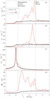 |
Fig. 2 Magnetic field and ion densities along the x axis at t = 76.8 s for cone angles α = 0° (black solid lines) and 90° (red dashed lines). (a) proton density np, (b) alpha particle density nα, (c) water ion density nW, and (d) the magnitude of the magnetic flux density |B|. The vertical lines show the locations of the diamagnetic cavity boundary and the bow shock. |
3.1.2 Parallel B
Figures 1e–h show the magnetic flux density and proton density in the x–z and x–y planes for the simulation run that has the IMF cone angle at α = 0°. In this case, there is no shock forming at all, and as a consequence there is no cometosheath either. A diamagnetic cavity forms around the nucleus, and extends downstream to the edge of the simulation box. Therefore, its true downstream extent cannot be determined in this simulation. There is no notable pile-up of the magnetic field in the subsolar region – unlike the α = 90° case – but the magnitude of the field peaks on the flanks, reaching 4.6 nT, which is higher than the IMF magnitude of 3.4 nT. This can be understood as a result of the formation of the diamagnetic cavity, which forces the magnetic flux to pass through the flanks instead of the centre of the comet.
The protons in the α = 0° case flow uninhibited into the inner coma, as there is no shock or any magnetic pile-up region to prevent it. The protons enter the diamagnetic cavity, and when they get close to the nucleus are deflected by the ambipolar electric field, forming a wake downstream, as can be seen in Figs. 1g and h. The ambipolar electric field is at its highest near the nucleus, as discussed in Sect. 3.2. The plasma is symmetric around the x axis in both fields and particle properties. Furthermore, in the absence of a bow shock, none of the structures indicative of waves and instabilities – that are present for α = 90° in the vicinity of the bow shock – exist in the α = 0° case.
Figure 2d shows that the magnetic flux density falls off gradually in 1 × 10³ ≤ x ≤ 2 × 10³ km and then declines faster for 0 ≤ x ≤ 1 × 10³ km. We use the same vertical line at x = 300 km to show the subsolar location of the diamagnetic cavity boundary for both the parallel and perpendicular IMF cases. In the parallel IMF case, this is where |B| ≈ 1 nT. In the perpendicular magnetic field case (red dashed line), |B| does not reach such low values because of the resistivity-limited dissipation discussed in Sect. 2. The densities of both the protons (Fig. 2a) and alpha particles (Fig. 2b) start to decline quickly at x ≈ 100 km – which is already inside the cavity – and reach the values they have in the wake, that is ~0.1 cm−3 for protons and ~0.02 cm−3 for alpha particles, near x = −400 km. The water ion density (Fig. 2c) peaks at the nucleus and dominates the plasma density in that region.
The plasma density gradient gives rise to an ambipolar electric field directed radially outward from the nucleus, which accelerates the water ions (e.g. Vigren & Eriksson 2017; Odelstad et al. 2018).
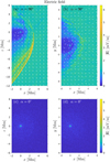 |
Fig. 3 Electric field magnitude E in the x–z and x–y planes at t = 76.8 s for cone angles α = 0° (black solid lines) and 90° (red dots). (a) |E| in the x–z plane for α = 90°, (b) |E| in the x–y plane for α = 90°, (c) |E| in the x–z plane for α = 0°, (d) |E| in the x–y plane for α = 0°. The arrows in panels a and b show the direction of the component of E that is in the plane shown. |
3.2 Electric field and ion motion
Figure 3 shows the magnitude of the electric field in the x–z and x–y planes for the two simulation runs. In all four panels, there is a peak in the electric field around the nucleus due to the ambipolar field generated by the density gradient. In the α = 90° case, there is also an enhanced electric field associated with the wave structure downstream of the bow shock that was discussed in Sect. 3.1.1. In the α = 0° case, the near-nucleus ambipolar field is the only notable contribution to the total electric field. Figure 4a shows the total electric field along the x axis for the two simulation runs, while Fig. 4b shows the ambipolar field:

and Fig. 4c shows the convective electric field:

where u is the bulk velocity of the ions. Figure 4d shows the Hall electric field:

and the resistive term of Eq. (1),

is shown in Fig. 4e. In the diamagnetic cavity, both the convective and Hall electric fields are negligible in both runs, regardless of the IMF clock angle. Therefore, the ambipolar electric field (Fig. 4b) is the only significant field in the diamagnetic cavity in both cases. For the case with α = 90°, the convective electric field dominates upstream, with the Hall field confined to values of below approximately half of the convective field. The numerical resistive electric field is small in comparison to the total electric field except at the location of the sharpest magnetic field gradient at x ≈ 500 km for the IMF cone angle α = 90° (see also Sects. 2 and 3.1.1).
How the electric and magnetic fields affect the motion of the ions can be seen in Fig. 5, which shows the υx and υz components of protons and water ions along the x axis for the two runs. In the simulation run with α = 90°, the υx component of the proton velocity becomes less negative as the solar wind protons move from x = 5 × 10³ km to x = 3 × 10³ km (Fig. 5a) and at the same time the υz component becomes more negative (Fig. 5b). In the same x range, the cometary water ions are picked up by the solar wind, obtaining a negative υx and a positive υz component (Figs. 5c and d) as they are accelerated by the convective electric field. This is due to mass-loading, which both decreases the magnitude of υ and deflects the solar wind ions in the direction opposite to the cometary ion motion, which means momentum can be conserved. At the bow shock, x ≈ 3 × 10³ km, the solar wind is slowed down substantially over a short distance, and closely downstream the wave structure that appears in B and np is also seen in υx and υz.
In the case of a parallel magnetic field, α = 0°, the proton υx component remains at the solar wind speed, except near the centre of the comet where it becomes less negative, as the protons are affected by the force from the ambipolar electric field (Fig. 5a). The υz component of the solar wind protons in Fig. 5b only shows insignificant fluctuations. Figure 5c shows the υx component of the cometary water ions. The ambipolar electric field is directed radially outward from the origin, and is therefore sunward for x > 0 and antisunward for x < 0. This means that the ions move away from x = 0 and are accelerated by the ambipolar electric field for small values of |x|, and further away from the comet centre the υx curve quickly becomes flat where the water ion density gradient starts to decline. As the right-hand side of the figure is approached (x = 5 × 10³ km), the water ion υx component has fallen back to zero. The ions accelerated near the nucleus have not had time to reach x = 5 × 10³ km at the end of the simulation run, and the ion population is dominated by local production. However, the water ion density at these distances is small, as Fig. 2 shows. Also, in the run with α = 90°, the water ions are accelerated by the ambipolar field. There, on the other hand, their υx component decreases and changes sign near x = 1 × 10³ km. This is due to the barrier created by the magnetic pile-up and by the presence of Hall and convective electric fields in that region. As the υx component changes sign, the ions turn around, and this causes the bump on the red dashed line in Fig. 2c where the water ion density is higher in the α = 90° than in the α = 0° case between x = 100 km and x = 750 km.
Figure 6 shows two-dimensional proton distribution functions in the diamagnetic cavity (left column, panels a and c) and a reference point upstream on the x axis (right column, panels b and d). The perpendicular velocity υ⊥ is the velocity component that is perpendicular to the x axis, and the distribution function (υx, υ⊥) is defined so that the integral
 (5)
(5)
yields the proton density. The distributions are computed based on the particles in a sphere of 200 km in radius centred on (x, y, z) = (0, 0, 0) for the diamagnetic cavity and (x, y, z) = (4.5 × 10³, 0, 0)km for the reference volume. Densities, bulk velocities, and temperatures for these distributions are shown in Table 2.
In the run with a perpendicular magnetic field, α = 90°, the protons already have a non-zero υ⊥ component when they are in the reference volume (Fig. 6b). This is due to the deflection in the negative z direction that is caused by mass-loading and starts already far upstream, and the same effect is driving the negative υz component in the reference volume for the α = 90° case, as shown in Table 2. Only three proton macro-particles entered the outskirts of the sphere where the particles for the distribution in the cavity were collected. The resulting density is negligible and is rounded off to 0.0 cm−3 in Table 2. No values for the velocity or temperature are given in the table for that case, as three macroparticles are insufficient to give statistically significant values.
In the run with a parallel magnetic field, α = 0°, the protons are slowed down in their x-directed motion by 60 km s−1, while they move from the reference volume to the diamagnetic cavity and encounter the ambipolar electric field. Comparing Fig. 6c to Fig. 6d, an increase in the perpendicular velocity component between the reference volume and the cavity is evident. This is caused by the radially directed ambipolar electric field, which deflects the protons away from the x axis as they come close to the nucleus.
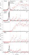 |
Fig. 4 Electric field along the x axis at t = 76.8 s for cone angles α = 0° (black solid lines) and 90° (red dots). (a) Magnitude of the total electric field. (b) Magnitude of the ambipolar electric field Ea = −∇pe/ρi. (c) Magnitude of the convective electric field Ec = −υ × B. (d) Magnitude of the Hall electric field EH = J × B/(nee). (e) Magnitude of the resistive contribution to the electric field Eres = ηJ. The vertical lines show the locations of the diamagnetic cavity boundary and the bow shock. |
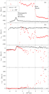 |
Fig. 5 Velocity components υx and υz along the x axis at t = 76.8 s for cone angles α = 0° and 90°. (a) proton x velocity component, υxp, (b) proton z velocity component, υzp, (c) water ion x velocity component, υxW, and (d) water ion z velocity component, υxW. The vertical lines show the locations of the diamagnetic cavity boundary and the bow shock. |
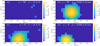 |
Fig. 6 Proton distribution functions (υx, υ⊥) – where υ⊥ is the velocity component perpendicular to the x axis – for cone angles α = 0° and 90°. (a) Inside the cavity for α = 90°, (b) in the upstream reference volume for α = 90°, (c) inside the cavity for α = 0°, (d) in the upstream reference volume for α = 0°. The distribution function is normalised so that the proton density is given by np = ∫∫ dυxdυ⊥. The distributions shown are the averages of two different time steps, namely t = 76.8 s and 80 s. |
4 Discussion and conclusions
We simulated the interaction between the solar wind and comet 67P for two cases, where in one case the IMF was parallel to the solar wind velocity and in the other the IMF was perpendicular to it. In both cases, the magnetic field drops significantly, forming a diamagnetic cavity, although B does not decrease all the way to zero because of the resistivity that was introduced to prevent numerical instabilities. In the case with a parallel IMF, solar wind ions were able to enter the diamagnetic cavity. In the case of a perpendicular IMF, all except a negligible fraction of the solar wind ions were deflected before reaching the cavity. This is in agreement with observations by the Rosetta spacecraft (Goetz et al. 2023), and also confirms the hypothesis made by Goetz et al. (2023) that a parallel IMF opens a path for solar wind ions to enter the diamagnetic cavity.
We included two solar-wind ion species in these simulations: protons and alpha particles. During parallel IMF, the two species behave in the same way, whereas for a perpendicular IMF, the scale length is longer for the alpha particles than for the protons when they are slowed down after the bow shock (Figs. 2a and b). The shapes of the density profiles for alpha particles and protons also differ to some extent. However, the density of the protons being much higher than that of the alpha particles, the protons are the solar wind species that is dominating the interaction with the comet.
In the case of a perpendicular IMF, a bow shock forms upstream of the nucleus, and on its downstream side is a come to sheath followed by a region where the magnetic field piles up and the solar wind ions are deflected so that a solar-wind ion cavity is created. The diamagnetic cavity is situated inside this solar-wind ion cavity. There is also an abundance of waves near the bow shock on its downstream side.
In the case of a parallel IMF, no bow shock forms and therefore there is no magnetosheath either, nor are there any of the waves associated with the bow shock. A solar wind ion wake forms downstream of the nucleus, because the solar wind ions are deflected by the ambipolar electric field as they pass through the near-nucleus region. The wake is located inside the diamagnetic cavity, at least as far as 2000 km downstream of the nucleus, which is where the simulation domain ends. How the diamagnetic cavity boundary closes on the nightside is not elucidated by this simulation in either of the two cases, and that side of the cavity has never been probed by spacecraft.
The fate of the cometary ions in the two different configurations is a matter of interest. In the case of a perpendicular IMF, the cometary ions are picked up by the solar wind via its convective electric field. When the IMF is parallel to the solar wind velocity, this electric field does not exist. In this case, the ions are accelerated outwards by the ambipolar electric field near the nucleus (Figs. 3 and 4), obtaining speeds that are much lower than the solar wind speed (Fig. 5); they then continue to move outward at that speed until the end of the simulation run. At a real comet in the solar wind, the ions would move slowly in this way either until the IMF direction changes, leading to their pickup by a convective electric field, or would be picked up via wave-particle interaction. This could for example involve Alfvén waves, as discussed by Huddleston & Johnstone (1992), but this would require length scales larger than what is considered in the simulations presented here. The timescale of the response of the comet to a change in the IMF direction could be studied in simulations, but that is beyond the scope of this article. However, it can be estimated from particle transit times. The transit time for solar wind ions through the entire simulation domain is approximately 1 min, which is about as long it takes for the initial transients to subside (cf. Sect. 2). The cometary ions are accelerated by the electric field. Inside the diamagnetic cavity, the electric field is not affected by the IMF orientation. Outside the cavity, cometary ion speeds are of the order of 10–20 km s−1 and they would therefore move out of the inner coma within a few minutes at most.
The scenario explaining the observations of solar wind protons in the diamagnetic cavity presented here is valid for comet 67P and could be extended to other comets with similar outgassing rates. For highly active comets, like comet 1P/Halley, we expect other phenomena to dominate. At comet 67P, as simulated here, there is no bow shock in the radial IMF situation, whereas for comet 1P/Halley a quasi-parallel shock was observed by both the Giotto and Vega 2 spacecraft (Galeev et al. 1986; Coates 1995). Also, charge-exchange collisions become important for a highly outgassing comet. Loss of solar wind ions due to charge exchange was observed by Rosetta at comet 67P (Simon Wedlund et al. 2019a,b, 2016), and charge-exchange effects become more pronounced as the outgassing rate increases. For a highly active comet, this could prevent solar wind ions from reaching the inner coma at all.
These simulations also provide some information on the nature of cometary tail disconnection events (DE), which is one of the outstanding questions in cometary plasma science (Goetz et al. 2022b). In remote optical observations of comets, the tail appears to be disconnected or broken during these events. Many mechanisms have been invoked to explain the sudden disruption of a cometary tail; for example, magnetic reconnection due to an encounter with an interplanetary sector boundary (Niedner Jr. & Brandt 1978) or the flute instability caused by an encounter with a solar-wind high-speed stream (Ip & Mendis 1978). Wegmann (1995) showed with magnetohydrodynamic simulations that a comet encountering an interplanetary shock could show signs of a DE, namely a reduction in cometary ion column density in the far tail. The simulations presented here show that when the comet encounters a solar-wind radial field, the pick-up of cometary ions is reduced and therefore no new cometary ions are incorporated into the solar wind flow. Thus, when the IMF turns radial at a comet, there will be a pause in the buildup of the ion tail, while the ions that have already been picked up continue their antisunward motion, leaving a gap behind them. When observing the column density during such an encounter, this should also lead to a reduction in visible cometary ions, which could appear as a DE. We can therefore add a solar-wind radial field to the long list of triggers of DE.
Hybrid simulations can be used to the model diamagnetic cavities seen here and in previous work (e.g. Koenders et al. 2015), and they can further our understanding of cometary–solar wind interaction in general and of specific problems, such as that treated in this paper. However, these simulations cannot account for all the related physical processes, as electrons are not treated kinetically. Kinetic simulations of the diamagnetic cavity boundary – including electrons – have been performed in a one-dimensional setup (Beth et al. 2022). However, both the Rosetta observations (Goetz et al. 2016b,a) and laboratory analogues of diamagnetic cavities (Schaeffer et al. 2022) indicate that the boundary of the diamagnetic cavity is both structured and dynamic in more than one dimension. Therefore, future work on a complete description that can explain the shape, structure, and causes of the cavity formation will require three-dimensional simulations where both ions and electrons are treated kinetically.
The direction of the IMF affects the interaction between the solar wind and all Solar System objects. Solar wind interaction with a comet under radial IMF shares many properties with solar wind interaction with the unmagnetised planets Mars (Fowler et al. 2022) and Venus (Chang et al. 2020). We expect future research of both planets and comets to advance our understanding of radial IMF conditions at unmagnetised objects in general.
Acknowledgements
The authors thank Arnaud Beth and Anja Moeslinger for valuable discussions. This work was supported by the Swedish National Space Agency contract 108/18. The simulations were performed in part using resources provided by the High Performance Computing Center North (HPC2N) at UmeåUniversity in Sweden; in part using hardware funded by Kempestiftelserna and a mid-range equipment grant from the Faculty of Science and Technology at Umeå University, Sweden; and the NVIDIA Academic Hardware Program. SF acknowledges financial support from SNSA grant 115/18 and the Swedish Research Council 2018-03454.
References
- Alho, M., Simon Wedlund, C., Nilsson, H., et al. 2019, A&A, 630, A45 [NASA ADS] [CrossRef] [EDP Sciences] [Google Scholar]
- Behar, E., Nilsson, H., Stenberg Wieser, G., et al. 2016, Geophys. Res. Lett., 43, 1411 [NASA ADS] [CrossRef] [Google Scholar]
- Behar, E., Nilsson, H., Alho, M., Goetz, C., & Tsurutani, B. 2017, MNRAS, 469, S396 [Google Scholar]
- Beth, A., Gunell, H., Wedlund, C. S., et al. 2022, A&A, 667, A143 [NASA ADS] [CrossRef] [EDP Sciences] [Google Scholar]
- Biermann, L., Brosowski, B., & Schmidt, H. U. 1967, Sol. Phys., 1, 254 [NASA ADS] [CrossRef] [Google Scholar]
- Chang, Q., Xu, X., Xu, Q., et al. 2020, ApJ, 900, 63 [Google Scholar]
- Coates, A. J. 1995, Adv. Space Res., 15, 403 [NASA ADS] [CrossRef] [Google Scholar]
- Deca, J., Divin, A., Henri, P., et al. 2017, Phys. Rev. Lett., 118, 205101 [Google Scholar]
- Deca, J., Henri, P., Divin, A., et al. 2019, Phys. Rev. Lett., 123, 055101 [Google Scholar]
- Divin, A., Deca, J., Eriksson, A., et al. 2020, ApJ, 889, L33 [NASA ADS] [CrossRef] [Google Scholar]
- Fatemi, S., Poppe, A. R., Delory, G. T., & Farrell, W. M. 2017, J. Phys. Conf. Ser., 837, 012017 [NASA ADS] [CrossRef] [Google Scholar]
- Fatemi, S., Poppe, A. R., Vorburger, A., Lindkvist, J., & Hamrin, M. 2022, J. Geophys. Res. Space Phys., 127, e2021JA029863 [CrossRef] [Google Scholar]
- Fowler, C. M., Hanley, K. G., McFadden, J., et al. 2022, J. Geophys. Res. Space Phys., 127, e2022JA030726 [NASA ADS] [CrossRef] [Google Scholar]
- Galeev, A. A., Gribov, B. E., Gombosi, T., et al. 1986, Geophys. Res. Lett., 13, 841 [NASA ADS] [CrossRef] [Google Scholar]
- Glassmeier, K.-H., Coates, A. J., Acuna, M. H., et al. 1989, J. Geophys. Res., 94, 37 [CrossRef] [Google Scholar]
- Glassmeier, K.-H., Boehnhardt, H., Koschny, D., Kührt, E., & Richter, I. 2007, Space Sci. Rev., 128, 1 [Google Scholar]
- Goetz, C., Koenders, C., Hansen, K. C., et al. 2016a, MNRAS, 462, S459 [NASA ADS] [CrossRef] [Google Scholar]
- Goetz, C., Koenders, C., Richter, I., et al. 2016b, A&A, 588, A24 [NASA ADS] [CrossRef] [EDP Sciences] [Google Scholar]
- Goetz, C., Gunell, H., Johansson, F., et al. 2021, Ann. Geophys., 39, 379 [NASA ADS] [CrossRef] [Google Scholar]
- Goetz, C., Behar, E., Beth, A., et al. 2022a, Space Sci. Rev., 218, 65 [NASA ADS] [CrossRef] [Google Scholar]
- Goetz, C., Gunell, H., Volwerk, M., et al. 2022b, Exp. Astron., 54, 1129 [NASA ADS] [CrossRef] [Google Scholar]
- Goetz, C., Scharré, L., Simon Wedlund, C., et al. 2023, J. Geophys. Res. Space Phys., 128, e2022JA031249 [NASA ADS] [CrossRef] [Google Scholar]
- Gombosi, T. I., Powell, K. G., & Zeeuw, D. L. D. 1994, J. Geophys. Res. (Space Phys.), 99, 21525 [NASA ADS] [CrossRef] [Google Scholar]
- Gunell, H., & Goetz, C. 2023, A&A, 674, A65 [NASA ADS] [CrossRef] [EDP Sciences] [Google Scholar]
- Gunell, H., Goetz, C., Simon Wedlund, C., et al. 2018, A&A, 619, A2 [NASA ADS] [CrossRef] [EDP Sciences] [Google Scholar]
- Gunell, H., Lindkvist, J., Goetz, C., Nilsson, H., & Hamrin, M. 2019, A&A, 631, A174 [NASA ADS] [CrossRef] [EDP Sciences] [Google Scholar]
- Haser, L. 1957, Bull. Soc. Roy. Sci. Liège, 43, 740 [Google Scholar]
- Heppner, J. P., Sugiura, M., Skillman, T. L., Ledley, B. G., & Campbell, M. 1967, J. Geophys. Res., 72, 5417 [NASA ADS] [CrossRef] [Google Scholar]
- Huddleston, D. E., & Johnstone, A. D. 1992, J. Geophys. Res. (Space Phys.), 97, 12217 [NASA ADS] [CrossRef] [Google Scholar]
- Ip, W. H., & Mendis, D. A. 1978, ApJ, 223, 671 [NASA ADS] [CrossRef] [Google Scholar]
- Johnstone, A. D. 1991, Cometary Plasma Processes, 61 (Washington DC: American Geophysical Union Geophysical Monograph Series) [Google Scholar]
- Koenders, C., Glassmeier, K.-H., Richter, I., Motschmann, U., & Rubin, M. 2013, Planet. Space Sci., 87, 85 [NASA ADS] [CrossRef] [Google Scholar]
- Koenders, C., Glassmeier, K.-H., Richter, I., Ranocha, H., & Motschmann, U. 2015, Planet. Space Sci., 105, 101 [Google Scholar]
- Koenders, C., Perschke, C., Goetz, C., et al. 2016, A&A, 594, A66 [NASA ADS] [CrossRef] [EDP Sciences] [Google Scholar]
- Lindkvist, J., Hamrin, M., Gunell, H., et al. 2018, A&A, 616, A81 [NASA ADS] [CrossRef] [EDP Sciences] [Google Scholar]
- Niedner Jr., M. B., & Brandt, J. C. 1978, ApJ, 223, 655 [NASA ADS] [CrossRef] [Google Scholar]
- Nilsson, H., Stenberg Wieser, G., Behar, E., et al. 2015, Science, 347, aaa0571 [NASA ADS] [CrossRef] [Google Scholar]
- Nilsson, H., Stenberg Wieser, G., Behar, E., et al. 2017, MNRAS, 469, S252 [Google Scholar]
- Nilsson, H., Gunell, H., Karlsson, T., et al. 2018, A&A, 616, A50 [NASA ADS] [CrossRef] [EDP Sciences] [Google Scholar]
- Odelstad, E., Eriksson, A. I., Johansson, F. L., et al. 2018, J. Geophys. Res. (Space Phys.), 123, 5870 [NASA ADS] [CrossRef] [Google Scholar]
- Scarf, F. L., Coroniti, F. V., Kennel, C. F., et al. 1986, Geophys. Res. Lett., 13, 857 [NASA ADS] [CrossRef] [Google Scholar]
- Schaeffer, D. B., Cruz, F. D., Dorst, R. S., et al. 2022, Phys. Plasmas, 29, 042901 [NASA ADS] [CrossRef] [Google Scholar]
- Simon Wedlund, C., Kallio, E., Alho, M., et al. 2016, A&A, 587, A154 [NASA ADS] [CrossRef] [EDP Sciences] [Google Scholar]
- Simon Wedlund, C., Alho, M., Gronoff, G., et al. 2017, A&A, 604, A73 [NASA ADS] [CrossRef] [EDP Sciences] [Google Scholar]
- Simon Wedlund, C., Behar, E., Kallio, E., et al. 2019a, A&A, 630, A36 [NASA ADS] [CrossRef] [EDP Sciences] [Google Scholar]
- Simon Wedlund, C., Behar, E., Nilsson, H., et al. 2019b, A&A, 630, A37 [NASA ADS] [CrossRef] [EDP Sciences] [Google Scholar]
- Tsurutani, B. T., & Smith, E. J. 1986a, Geophys. Res. Lett., 13, 263 [NASA ADS] [CrossRef] [Google Scholar]
- Tsurutani, B. T., & Smith, E. J. 1986b, Geophys. Res. Lett., 13, 259 [NASA ADS] [CrossRef] [Google Scholar]
- Tsurutani, B. T., & Oya, H., eds. 1989, Plasma Waves and Instabilities at Comets and in Magnetospheres (Washington, DC: American Geophysical Union Geophysical Monograph Series), 53 [Google Scholar]
- Vigren, E., & Eriksson, A. I. 2017, AJ, 153, 150 [NASA ADS] [CrossRef] [Google Scholar]
- Wegmann, R. 1995, A&A, 294, 601 [NASA ADS] [Google Scholar]
In this paper, the inner coma is the region where the plasma is dominated by cometary species.
All Tables
All Figures
|
Fig. 1 Magnetic flux density and proton density in the x–z and x–y planes at t = 76.8 s for cone angles α = 0° and 90°. (a) |B| in the x–z plane for α = 90°, (b) |B| in the x–y plane for α = 90°, (c) np in the x–z plane for α = 90°, (d) np in the x–y plane for α = 90°, (e) |B| in the x–z plane for α = 0°, (f) |B| in the x–y plane for α = 0°, (g) np in the x–z plane for α = 0°, and (h) np in the x–y plane for α = 0°. The cross symbol (×) marks the position of the nucleus. In the magnetic field panels, the arrows show the direction of the component of B in the plane shown. In the proton density panels, the arrows show the direction of the proton bulk velocity component in the plane shown. |
| In the text | |
|
Fig. 2 Magnetic field and ion densities along the x axis at t = 76.8 s for cone angles α = 0° (black solid lines) and 90° (red dashed lines). (a) proton density np, (b) alpha particle density nα, (c) water ion density nW, and (d) the magnitude of the magnetic flux density |B|. The vertical lines show the locations of the diamagnetic cavity boundary and the bow shock. |
| In the text | |
|
Fig. 3 Electric field magnitude E in the x–z and x–y planes at t = 76.8 s for cone angles α = 0° (black solid lines) and 90° (red dots). (a) |E| in the x–z plane for α = 90°, (b) |E| in the x–y plane for α = 90°, (c) |E| in the x–z plane for α = 0°, (d) |E| in the x–y plane for α = 0°. The arrows in panels a and b show the direction of the component of E that is in the plane shown. |
| In the text | |
|
Fig. 4 Electric field along the x axis at t = 76.8 s for cone angles α = 0° (black solid lines) and 90° (red dots). (a) Magnitude of the total electric field. (b) Magnitude of the ambipolar electric field Ea = −∇pe/ρi. (c) Magnitude of the convective electric field Ec = −υ × B. (d) Magnitude of the Hall electric field EH = J × B/(nee). (e) Magnitude of the resistive contribution to the electric field Eres = ηJ. The vertical lines show the locations of the diamagnetic cavity boundary and the bow shock. |
| In the text | |
|
Fig. 5 Velocity components υx and υz along the x axis at t = 76.8 s for cone angles α = 0° and 90°. (a) proton x velocity component, υxp, (b) proton z velocity component, υzp, (c) water ion x velocity component, υxW, and (d) water ion z velocity component, υxW. The vertical lines show the locations of the diamagnetic cavity boundary and the bow shock. |
| In the text | |
|
Fig. 6 Proton distribution functions (υx, υ⊥) – where υ⊥ is the velocity component perpendicular to the x axis – for cone angles α = 0° and 90°. (a) Inside the cavity for α = 90°, (b) in the upstream reference volume for α = 90°, (c) inside the cavity for α = 0°, (d) in the upstream reference volume for α = 0°. The distribution function is normalised so that the proton density is given by np = ∫∫ dυxdυ⊥. The distributions shown are the averages of two different time steps, namely t = 76.8 s and 80 s. |
| In the text | |
Current usage metrics show cumulative count of Article Views (full-text article views including HTML views, PDF and ePub downloads, according to the available data) and Abstracts Views on Vision4Press platform.
Data correspond to usage on the plateform after 2015. The current usage metrics is available 48-96 hours after online publication and is updated daily on week days.
Initial download of the metrics may take a while.