| Issue |
A&A
Volume 631, November 2019
|
|
|---|---|---|
| Article Number | A170 | |
| Number of page(s) | 6 | |
| Section | Interstellar and circumstellar matter | |
| DOI | https://doi.org/10.1051/0004-6361/201935993 | |
| Published online | 18 November 2019 | |
Numerical models for the dust in RCW 120
1
LUTH, Observatoire de Paris, PSL, CNRS, UMPC, Université Paris Diderot,
5 place Jules Janssen,
92195
Meudon,
France
e-mail: This email address is being protected from spambots. You need JavaScript enabled to view it.
2
Instituto de Ciencias Nucleares, Universidad Nacional Autónoma de México,
Ap. 70-543,
04510
D.F.,
México
3
Aix-Marseille Université, CNRS, Laboratoire d’Astrophysique de Marseille,
13388
Marseille Cedex 13,
France
Received:
31
May
2019
Accepted:
30
July
2019
Abstract
Context. The interstellar bubble RCW 120 seen around a type O runaway star is driven by the stellar wind and the ionising radiation emitted by the star. The boundary between the stellar wind and interstellar medium (ISM) is associated with the arc-shaped mid-infrared dust emission around the star within the HII region.
Aims. We aim to investigate the arc-shaped bow shock in RCW 120 by means of numerical simulations, including the radiation, dust, HII region, and wind bubble.
Methods. We performed 3D radiation-hydrodynamic simulations including dust using the GUACHO code. Our model includes a detailed treatment of dust grains in the ISM and takes into account the drag forces between dust and gas and the effect of radiation pressure on the gas and dust. The dust is treated as a pressureless gas component. The simulation uses typical properties of RCW 120. We analyse five simulations to deduce the effect of the ionising radiation and dust on both the emission intensity and the shape of the shock.
Results. The interaction of the wind and the ionising radiation from a runaway star with the ISM forms an arc-shaped bow shock where the dust from the ISM accumulates in front of the moving star. Moreover, the dust forms a second small arc-shaped structure within the rarefied region at the back of the star inside the bubble. In order to obtain the decoupling between the gas and the dust, it is necessary to include the radiation-hydrodynamic equations together with the dust and the stellar motion. In this work all these elements are considered together, and we show that the decoupling between gas and dust obtained in the simulation is in agreement with the morphology of the infrared observations of RCW 120.
Key words: ISM: bubbles / HII regions / ISM: individual objects: RCW120 / dust, extinction
© A. Rodríguez-González et al. 2019
 Open Access article, published by EDP Sciences, under the terms of the Creative Commons Attribution License (http://creativecommons.org/licenses/by/4.0), which permits unrestricted use, distribution, and reproduction in any medium, provided the original work is properly cited.
1 Introduction
The Infrared Astronomical Satellite (IRAS, Neugebauer et al. 1984) all-sky survey detected many extended arc-like structures associated with OB-runaway stars and paved the way for further studies to reveal the bow shocks that are present around these powerful stellar winds (van Buren et al. 1995; Peri et al. 2012). Furthermore, the mid-infrared (MIR) observations from Spitzer-MIPSGAL (Carey et al. 2009) of interstellar bubbles along the Galactic plane show that the interiors of HII regions contain dust, and some of them present 24 μm dust emission near to the central ionising source (Deharveng et al. 2010; Kendrew et al. 2012; Simpson et al. 2012). The dust grains are expected to evacuate the interiors of the hot bubbles as a result of the mechanical energy and radiation injected by the massive stars. However, recently, infrared observations show a significant amount of dust in the inner part of the bubble, particularly sitting near to the stellar feedback source. Indeed, high-resolution infrared observations show that HII bubbles contain a significant amount of dust in their interiors (Deharveng et al. 2010; Martins et al. 2010; Anderson et al. 2012). Everett & Churchwell (2010) explored the possibility that the evaporation of small dense cloudlets could resupply the hot gas with a new generation of dust grains. While this mechanism can explain the presence of dust inside HII bubbles, it is not capable of producing the morphology of the MIR radiation: an arc-shaped and a peaking close to the ionising source. (Ochsendorf et al. 2014, see also van Buren & McCray 1988) proposed that dust grains are expelled from ionised stars by radiation pressure and Pavlyuchenkov et al. (2013) performed 1D numerical calculations on the dust in the boundary between the stellar wind and the interstellar medium (ISM), and they concluded that dust deviation by itself is not a viable mechanism to adequately explain the arcs observed in 24 μm IR emission in HII regions. One of the more studied interstellar bubbles with a 24 μm arc is RCW 120. The RCW 120 bubble is located at 1.3 kpc (Zavagno et al. 2007) at l = 348. °3, b = +0. °5 (αJ200 = 17h09m0s, δJ200 = −38°24′ (Rodgers et al. 1960) with a radius of 1.9 pc (Anderson et al. 2015). Its ionising star is CD-38°11636 or LSS 3959, an O8 type star (Georgelin & Georgelin 1970; Avedisova & Kondratenko 1984; Russeil 2003; Zavagno et al. 2007) located at αJ200 = 17h12m20.6s, δJ200 = −38°29′26″. This star is found in a Galactic HII region embedded in a molecular cloud with numerical density of na ~ 3000 cm−3 (Zavagno et al. 2007). The age of the massive star is <3 Myr, and the dynamical age of the shell is ~0.2 Myr (Arthur et al. 2011). More recently, Torii et al. (2015) found that the dynamical age is ~0.4 Myr. Ochsendorf et al. (2014) proposed a pressure and density gradient in the ISM around the ionising source of RCW 120, in order to explain the asymmetry of the HII region and the MIR arcs. However the diameter of the RCW 120 is around 3.8 pc (Anderson et al. 2015) and a pressure or density gradient must be related to a stellar motion (Weaver et al. 1977; Raga 1986; Mac Low et al. 1991; Arthur & Hoare 2006; Mackey et al. 2013; Steggles et al. 2017). Most probably, the stars, particularly the massive stars, are born in motion with respect to their surroundings because they keep the momentum gained during their star formation process, where the turbulence is needed, with velocities of 2−5 km s−1 (e.g., Peters et al. 2010; Dale & Bonnell 2011).
Many authors have modelled bow shocks from runaway O and B stars (e.g. Mac Low et al. 1991; Comeron & Kaper 1998; Meyer et al. 2014) and there have been a few studies of HII regions for v ≥ 20 km s−1, (Tenorio-Tagle 1979; Raga et al. 1997; Mackey et al. 2013). In both cases a partial shocked shell forms, upstream for the bow shock and in the lateral direction for the HII region, and can be unstable in certain circumstances. In the case of RCW 120, Mackey et al. (2016) performed 2D radiation hydrodynamical numerical simulations of stellar wind bubbles and post-processing calculations to obtain synthetic intensity maps at infrared wavelengths. They found good agreement between their model and the RCW 120 observations. In particular, they obtained an infrared arc with the same shape and size as the arc observed in RCW 120, with a brightness comparable to the observed one. They concluded that their results could be showing the outer edges of an asymmetric stellar wind bubble. On the other hand, the respective effects of the smaller and larger dust grains has been studied by van Marle et al. (2011). These latter authors modelled the gas and dust dynamics using high-resolution numerical simulations of a fast-moving red supergiant and concluded that the smaller sized grains follow the motion of the gas and the larger grains are weakly coupled to the gas. Therefore, they proposed that the small dust grains dominate the emission in the infrared observations. Moreover, De Colle & Raga (2006) and Meyer et al. (2017) showed that a small magnetic field can affect the predicted emission from the post-shock recombination regions by one or two orders of magnitude. However, the work of these latter authors was focused on the optical emission prescriptions and they did not study the infrared emission mainly produced by the dust grains. Indeed, Meyer et al. (2017) made post-processing calculations of the dust continuum infrared emission and showed that the presence of the magnetic field decreases the infrared emission. Finally, using 3D magneto-hydrodynamical simulations Katushkina et al. (2018) showed that the drag force cannot be neglected in models with ISM densities larger than 10 cm−3.
More recently, Henney & Arthur (2019a,b,c), studied the formation of IR-emission arcs around luminous stars that move supersonically relative to their surrounding medium. These latter authors found four different regimes depending on the type of coupling between dust grains and gas, and taking into consideration the relative values between the stellar wind and the ultraviolet optical depth of the bow shell. They presented cases in which a radiation-supported dust wave decouples from the gas to form an infrared emission arc outside of any hydrodynamic bow shock, considering the magnetic fields in their numerical models. They considered the drag force because of the dust and the gas interactions assuming that the fraction of the dust is zero in the wind.
In the present study, we modelled the RCW 120 physical properties, performing a series of numerical simulations that solve the radiation-hydrodynamics and dust equations in a fully 3D fixed Cartesian mesh. This paper is organized as follows: the numerical simulation setup is described in Sect. 2, the simulation results are presented in Sect. 3, and finally we conclude in Sect. 4.
2 Governing equations
We performed 3D simulations using the Guacho1 code (Esquivel et al. 2009; Esquivel & Raga 2013). The Guacho code uses a Cartesian grid to solve the near-conservation laws governing the gas-dynamics and the neutral hydrogen rate. It includes the radiative transfer at the Lyman limit of ionising photons emitted from an isotropic point source photoionising a neutral hydrogen distribution. Also, it uses the ray-tracing scheme where the diffuse radiation is considered only in the B recombination case. The code is described in detail in Esquivel & Raga (2013) and in Schneiter et al. (2016). In this project we incorporate the dust-grain dynamics coupled to gas dynamics and the momentum feedback of radiation on the dust.
The radiative cooling is included as described by Raga & Reipurth (2004) for the atomic gas, and for lower temperatures we have included the parametric molecular cooling function presented by Kosiński & Hanasz (2007) and Rivera-Ortiz et al. (2019). The complete set of equations is as follows:
![Mathematical equation: \begin{eqnarray} && \hspace*{-6pt} \frac{\partial \rho}{\partial t}+\vec{\nabla} \cdot \left(\rho\,\vec{v}\right)=0,\\ && \hspace*{-6pt} \frac{\partial \rho v}{\partial t}+\vec{\nabla} \cdot \left(\rho \,\vec{v}\cdot \vec{v}+p\right)=\rho\,f_{\textrm{rad}},\, \textrm{nHI}+f_{\textrm{d}},\\ && \hspace*{-6pt} \frac{\partial e }{\partial t} +\vec{\nabla}\cdot \left[\vec{v} \left(e+p\right) \right] =G_{\textrm{rad}}-L_{\textrm{rad}}+f_{\textrm{rad,nHI}}\;\vec{v} \,+\,f_{\textrm{d}}\,\vec{v},\\ && \hspace*{-6pt} \frac{\partial \rho_{\textrm{d}}}{\partial t}+\nabla \left(\rho_{\textrm{d}}\vec{v_{\textrm{d}}}\right)=0,\\ && \hspace*{-6pt} \frac{\partial \rho_{\textrm{d}} v_{\textrm{d}}}{\partial t}+ \nabla(\rho_{\textrm{d}} \vec{v_{\textrm{d}}}\cdot \vec{v_{\textrm{d}}})=\rho_{\textrm{d}} f_{\textrm{rad,d}}\,-\,f_{\textrm{d}}, \end{eqnarray}](/articles/aa/full_html/2019/11/aa35993-19/aa35993-19-eq1.png)
where, ρ, v, p, and E are the density, the velocity, the thermal pressure and the total energy density of the gas, respectively. Grad and Lrad are the energy gains and losses due to radiation. We assume a standard ideal gas law for closure, and therefore the gas total energy density and the gas thermal pressure are related by E = ρv2∕2 + P∕(γ − 1), where the ratio between specific capacities is γ = 5∕3.
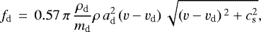
The factors ρd and vd are the density and the velocity of the dust. The drag force fd is given by a combination of Epstein’s drag law for the subsonic regime and Stokes’ drag law for the supersonic regime (see, van Marle et al. 2011),
 (6)
(6)
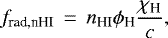
where  is the gas sound speed. The test of the hydrodynamics equation coupled with dust using the drag forces in Eq. (6) shows the same results as those obtained by van Marle et al. (2011). Finally, the radiation pressure gradient force due to photoionisation is
 (7)
(7)
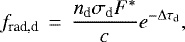
and the radiation pressure gradient force due to grain dust absorption is
 (8)
(8)
where ϕH is the Lyman α photoioinzation rate, χH is the hydrogen ionization potential, σd is the grain dust cross-section (the geometrical cross section), F* is the photons flux, and c is the light speed. More details about the radiative force are given in Rodríguez-Ramírez et al. (2016).
In the ray tracing scheme, the photon package emitted by an isotropic point source decays by a factor of  when travelling through neutral gas and dust. Along a path-length Δl, the opacities induced by neutral gas and dust are ΔτH = a0 nHI Δl and Δτd = ad ndΔl, respectively. Here, a0 is the photoionisation cross-section constant, ad is the geometrical dust cross-section, and nHI and nd are the HI and dust number density. The photoionisation rate ϕHI is computed by equating the ionising photon rate, S, to the ionization per unit time in each cell, that is, S = nHIϕHIdV.
Characteristics and parameters of the simulations.
Simulation parameters and setup
The coupled gas–dust and radiation pressure equations are advanced using the HLL scheme from Harten et al. (1983) with the second-order spatial re-construction minmod slope limiter coupled with the second-order time step.
The presented hydrodynamical simulations (Table 1) are carried in a Cartesian grid with a physical domain ![Mathematical equation: $\left[x,y,z\right]\, \in\,\left[\left(0,3\right)\!,\left(0,3\right)\!,\left(0,9\right)\right] \textrm{pc}$](/articles/aa/full_html/2019/11/aa35993-19/aa35993-19-eq7.png) with a spatial resolution of0.03 pc in each direction.
with a spatial resolution of0.03 pc in each direction.
The ISM has a uniform number density of na =3000 cm−3, temperature T0 = 100 K, and is moving in the z direction with a velocity of 5 km s−1 (to emulate the stellar motion of RCW 120). Our numerical models considered appropriate values of the stellar wind velocity (2300 km s−1) and a mass injection rate (2.7 × 10⁻⁷ M⊙ yr−1) for one single O8V star (Sternberg et al. 2003). The steady spherical stellar wind was imposed in a sphere of radius 0.09 pc at the simulation grid centre.
We used a photon ionisation rate of 1.6 × 1048 phot s−1 (see Zavagno et al. 2007) and the photons are injected in the surface of a sphere with a radius of 1.5 times the wind source radius.
We assume the dust to be composed of silicates, for which the internal particle density is ρgrain = 3.3 g cm−3 (Draine & Lee 1984). Concerning the dust shape, we assume spherical grains with a radius of adust. The simulations are performed with two dust radii, adust = 0.1 and adust = 1 μm. The dust to gas fraction is 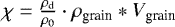 , where Vgrain is the volume of the grains. The dust is only included into the uniform ISM.
We computed simulations of RCW 120, varying the dust fraction and size, the momentum of the wind, the number of ionising photons, and the density in the ISM (see Table 1). Following Sánchez-Cruces et al. (2018) and Torii et al. (2015), we ran our simulations up to a time of 0.4 Myr.
3 The gas and dust decoupling
To understand the stellar wind and the photon pressure effect in the gas and dust dynamics and the dust–gas interaction, we performed five numerical models (Table 1). A cut in the Z− X plane of the model M3 is shown in Fig. 1. As we can see, two shock regions are formed: one strong shock in front of the runaway star, the nearest one; and the second, a weaker shock behind the runaway star. In the tail of the HII region, the cometary HII region, the shock wave forms a shell of less-dense, shocked ISM.
In order to analyse the behaviour of these two regions, we show in Fig. 2 a 1D cutalong two directions: a cut perpendicular to the moving star direction, the X-axis, and a cut in the moving direction, the Z-axis; at time 0.4 Myr (left an right panels of Fig. 2, respectively). It is clear that the two regions mentioned above are observed. For the M1 model, where only the stellar wind is considered without including the photons flux (the diamonds line in Fig. 2), the gas and dust are well coupled and are stacked at the external shell. Inside the bubble within the shell of the shocked ISM, there is a rarefied region with low gas and dust density. However, the gas is hot in this region. In Fig. 3 we show the fraction of ionised gas for cuts on the X and Z axes (left and right panels, respectively). In the cut on the X axis, one can see that the gas is completely ionised within a narrow region where the ram pressure and the over-pressure of the hot bubble reach equilibrium. This bubble of ionised (hot) gas is much larger in the Z direction than in the X-axis (1.2 pc.), namely about 3 pc extending in an opposite direction to the movement of the star, giving the cometary shape in this region. For this model, the ionised region has an ellipsoidal (egg-like) shape. In the other models, M2-M5, the ionising photons are included (Table 1). In those models, the ISM is heated by the ionization front which decreases the shock Mach number resulting in a lower compression in the external shell. At the tail of the cometary HII region only a compression wave forms and the shock remains only at the front and the side of the runaway star (Fig. 2). As a result, at the back of the moving star inside the bubble, the density increases and the temperature decreases. Models M3-M4, with dust in ISM and photoionisation, show a greater difference behind the runaway star inside the bubble, where more ISM gas and dust remains. Indeed, the dust decreases the compression wave strength. Moreover, the structure of this rarefied zone changes under the effect of the dust (Fig. 2). There is an increment in the gas density to 0.25 pc from the star and a minimum (local) at 1 pc for M3 and M4 models in comparison with 1.1 pc for the M2 model. Concerning the dust distribution in the M1, M3, M4, and M5 models, in front of the runaway star (Fig. 2) the compression shock is strong and the dust is tightly coupled with the gas. However, inside the bubble at the back of the runaway star in the rarefied region the dust is decoupled from the gas. This decoupling between thedust and gas is more important in model M3 because the dust grains are bigger. In models M3 and M4 there are zones where the dust accumulates. The denser zone is at the forward shock and the second is inside the bubble in the rarefied region (Fig. 2). As a result, there are two regions with a significant dust grain emission: (a) an outer region of swept up ISM and (b) a region more internal and close to the ionising star, at approximately 0.2 pc, which is formed with ISM gas filling the decreased pressure region due to the star motion.
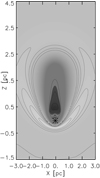 |
Fig. 1 Two-dimensional cut in the Z–X plane of the density contour in grey and dust contour with continuous lines. |
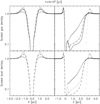 |
Fig. 2 Scaled gas density (upper panels) and scaled dust density (lower panels) along the X-axis (perpendicular to the direction of star propagation) and Z-axis (along the moving direction), at 0.4 Myr. The diamonds correspond to the M1 model, the solid, dotted, and dashed lines correspond to models M2, M3, and M4, and the triangles are for the M5 model, respectively. |
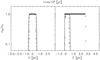 |
Fig. 3 Ionisation fraction for the M1, M2, M3, and M4 models at 0.4 Myr for a cut on the X and Z axes (left and right panel, respectively) in the centre of the simulation box. Lines and symbols are as in Fig. 2. |
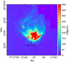 |
Fig. 4 RCW 120 image at 24 μm from Spitzer-MIPSGAL (Carey et al. 2009), showing emission of small dust grains heated by the stellar radiation. |
4 Dust distribution in RCW 120
A visual comparison of our models is described in this section. Figure 4 shows the emission of the Galactic RCW 120 bubble at 24 μm from Spitzer-MIPSGAL Carey et al. (2009). MIPSGAL is a survey of the same region as Spitzer-GLIMPSE surveys (see Churchwell et al. 2009 for more details) using the Multi-band Imaging Photometer for Spitzer (MIPS; Rieke et al. 2004) instrument at 24 μm. The MIPSGAL resolution is 6″ at 24 μm. This image shows the extended emission of small dust grains at 24 μm in the region of the ionised gas and the emission in the envelope associated with young stellar objects (YSOs). As one can see, the emission at 24 μm of dust is mainly localised in two places: (a) in an external and thin shell in the front part of the cometary HII region, and (b) near the ionising source in a central region of the bubble that has a significant dust fraction. Figure 1 shows a cut on the X–Y axis for the M3 model; the grey map is the gas density and the dust density contours. The blue contours correspond to the normalized density of dust larger or equal to 0.8 (the outer shell) and the contour corresponds to densities lower than 0.8 (the inner dust structure). As we can see in the Fig. 1, the HII region has an ellipsoidal (egg-like) structure and does not look like a spherical shape as shown in the observation in Fig. 4. In addition, although the distribution of the dust is in the external shell, because it was dragged by the leading shock, it is also seen that the internal structure of dust is behind the position of the source (marked with an asterisk in Fig. 1). Marsh & Whitworth (2019) determined the shape of the external shell of RCW 120 and concluded that it is a circular, and not elongated, ring with an internal radius of 1.66 pc and a depth of 0.33 pc. The elongation presented in the current numerical models with a star motion cannot explain the shape of the RCW 120. Torii et al. (2015) studied the proper motion in RCW 120 and found a problem with the determination of the molecular shell velocity with respect to the observer. It is therefore likely that the object has a projection angle that does not allow us to see an elongated shape in this HII region. Finally, in order to compare our model with observations, we built column density maps,  , where a rotation has been included. Figure 5 shows the column density for the dust for a rotating angle of 72 degrees of the projection plane X–Z. If the line of vision is perpendicular to the axis of movement, the external shell has the shape of a ring, with the ionising star at the centre of it. However, the rotation of 72 degrees that we have used results in an external shell with a spherical section in the direction of the movement of the star. Also, the internal region with dust now coincides with the position of the star.
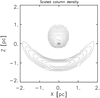 |
Fig. 5 Projection plane X–Z image of the scaled column density. Contours represent the scale column density for dust. The contours around the star have values around 0.1, while in the shell the rank is between 1.65 and 2.0 |
5 Conclusions
We present several numerical models for the evolution of the HII region, RCW 120. Our models consider the photoionisation effect, the wind injected by the central star, and the effect of dust on the dynamical evolution of this object and the stellar motion.
With respect to the M1 model, (without photoionisation), the gas and dust do not seem to uncouple, since they are dragged by the leading shock and both of them are stacked in an external shell. We performed a numerical simulation for a weak wind model (where the stellar wind transfers a momentum reduced by a factor of 100 compared with the other models). This model, M5, produces a bubble with gas and dust and a significant decoupling of the dust and gas is not seen.
Our strong stellar winds models show an internal region with a high density of gas and dust very close to the central star. On the other hand, the distribution of dust and gas inside the bubble is different, with a partial decoupling between them. The model in which thedust grains are smaller maintains the coupling or partially coupling of gas and dust for a longer time despite the interactions with the ionisation and shock fronts. The decoupling is greater in models M3 and M4, with larger dust grains 1 μm. In these models, the dust is mainly concentrated in the external shell and in the central structure near the position of the star. That is, the gas and dust density profiles are found with a very similar distribution as inside the RCW 120 bubble.
We show that when making a rotation of 72 degrees, the morphology results in an external shell with a spherical ring shape. Surprisingly, the internal region with dust now coincides with the position of the star. This coincides with the observations which suggest thatthere is an angle with respect to the line of sight that presents us from observing an elongated shape in RCW 120.
As far as we are aware, this is the first time that 3D gas-dynamic equations, coupled with the photoionisation and the dust together with the stellar motion, have been solved for RCW 120. Therefore, according to our models, all of these are of great importance to understand the distribution of dust in the RCW 120 bubble.
Our results show good agreement with those obtained by Mackey et al. (2016), and are in accordance with the general analysis of Henney & Arthur (2019b) for the case of a dust wave where the dust is decoupled from the gas. Indeed, the distribution of dust is mainly located in a region found immediately after the bow shock, as in the two works mentioned previously.
We highlight the fact that we have not included the magnetic field in our simulations coupled with radiation hydrodynamics and dust, and that this is important in order to compute synthetic maps with optical and infrared emission. The inclusion of the magnetic field in simulations and the effect of this on the emission is left for future work.
Finally, we have shown the importance of strong stellar wind in the decoupling of the gas and dust during the lifetime of the bubble.
Acknowledgements
We acknowledge support from DGAPA-UNAM grants IN-109518 and IG-100218. A.R.G. is grateful DGAPA-UNAM and CONACyT for the grants during a sabbatical stay in LUTH, Observatoire de Paris, and also is grateful to LUTH, Observatoire de Paris for their hospitality. Z.M. is grateful for the use of the High Performance Computing OCCIGEN CINES within the DARI project A0030406842.
References
- Anderson, L. D., Zavagno, A., Deharveng, L., et al. 2012, A&A, 542, A10 [NASA ADS] [CrossRef] [EDP Sciences] [Google Scholar]
- Anderson, L. D., Deharveng, L., Zavagno, A., et al. 2015, ApJ, 800, 101 [NASA ADS] [CrossRef] [Google Scholar]
- Arthur, S. J., & Hoare, M. G. 2006, ApJS, 165, 283 [NASA ADS] [CrossRef] [Google Scholar]
- Arthur, S. J., Henney, W. J., Mellema, G., de Colle, F., & Vázquez-Semadeni, E. 2011, MNRAS, 414, 1747 [NASA ADS] [CrossRef] [Google Scholar]
- Avedisova, V. S., & Kondratenko, G. I. 1984, Nauchnye Informatsii, 56, 59 [NASA ADS] [Google Scholar]
- Carey, S. J., Noriega-Crespo, A., Mizuno, D. R., et al. 2009, PASP, 121, 76 [NASA ADS] [CrossRef] [Google Scholar]
- Churchwell, E., Babler, B. L., Meade, M. R., et al. 2009, PASP, 121, 213 [NASA ADS] [CrossRef] [Google Scholar]
- Comeron, F., & Kaper, L. 1998, A&A, 338, 273 [NASA ADS] [Google Scholar]
- Dale, J. E., & Bonnell, I. 2011, MNRAS, 414, 321 [NASA ADS] [CrossRef] [Google Scholar]
- De Colle, F., & Raga, A. C. 2006, A&A, 449, 1061 [NASA ADS] [CrossRef] [EDP Sciences] [Google Scholar]
- Deharveng, L., Schuller, F., Anderson, L. D., et al. 2010, A&A, 523, A6 [NASA ADS] [CrossRef] [EDP Sciences] [Google Scholar]
- Draine, B. T.,& Lee, H. M. 1984, ApJ, 285, 89 [Google Scholar]
- Esquivel, A., & Raga, A. C. 2013, ApJ, 779, 111 [NASA ADS] [CrossRef] [Google Scholar]
- Esquivel, A., Raga, A. C., Cantó, J., & Rodríguez-González, A. 2009, A&A, 507, 855 [NASA ADS] [CrossRef] [EDP Sciences] [Google Scholar]
- Everett, J. E.,& Churchwell, E. 2010, ApJ, 713, 592 [NASA ADS] [CrossRef] [Google Scholar]
- Georgelin, Y. P., & Georgelin, Y. M. 1970, A&AS, 3, 1 [NASA ADS] [Google Scholar]
- Harten, A., Lax, P. D., & van Leer, B. 1983, J. SIAM Rev., 25, 35 [Google Scholar]
- Henney, W. J., & Arthur, S. J. 2019a, MNRAS, 486, 3423 [Google Scholar]
- Henney, W. J., & Arthur, S. J. 2019b, MNRAS, 486, 4423 [NASA ADS] [CrossRef] [Google Scholar]
- Henney, W. J., & Arthur, S. J. 2019c, MNRAS, 489, 2142 [NASA ADS] [CrossRef] [Google Scholar]
- Katushkina, O. A., Alexashov, D. B., Gvaramadze, V. V., & Izmodenov, V. V. 2018, MNRAS, 473, 1576 [NASA ADS] [Google Scholar]
- Kendrew, S., Simpson, R., Bressert, E., et al. 2012, ApJ, 755, 71 [NASA ADS] [CrossRef] [Google Scholar]
- Kosiński, R., & Hanasz, M. 2007, MNRAS, 376, 861 [NASA ADS] [CrossRef] [Google Scholar]
- Mac Low, M.-M., van Buren, D., Wood, D. O. S., & Churchwell, E. 1991, ApJ, 369, 395 [NASA ADS] [CrossRef] [Google Scholar]
- Mackey, J., Langer, N., & Gvaramadze, V. V. 2013, MNRAS, 436, 859 [NASA ADS] [CrossRef] [Google Scholar]
- Mackey, J., Haworth, T. J., Gvaramadze, V. V., et al. 2016, A&A, 586, A114 [NASA ADS] [CrossRef] [EDP Sciences] [Google Scholar]
- Marsh, K. A.,& Whitworth, A. P. 2019, MNRAS, 483, 352 [NASA ADS] [CrossRef] [Google Scholar]
- Martins, F., Pomarès, M., Deharveng, L., & Zavagno, A., & Bouret, J. C. 2010, A&A, 510, A32 [NASA ADS] [CrossRef] [EDP Sciences] [Google Scholar]
- Meyer, D. M. A., Mackey, J., Langer, N., et al. 2014, MNRAS, 444, 2754 [NASA ADS] [CrossRef] [Google Scholar]
- Meyer, D. M. A., Mignone, A., Kuiper, R., Raga, A. C., & Kley, W. 2017, MNRAS, 464, 3229 [NASA ADS] [CrossRef] [Google Scholar]
- Neugebauer, G., Habing, H. J., van Duinen, R., et al. 1984, ApJ, 278, L1 [Google Scholar]
- Ochsendorf, B. B., Cox, N. L. J., Krijt, S., et al. 2014, A&A, 563, A65 [NASA ADS] [CrossRef] [EDP Sciences] [Google Scholar]
- Pavlyuchenkov, Y. N., Kirsanova, M. S., & Wiebe, D. S. 2013, Astron. Rep., 57, 573 [NASA ADS] [CrossRef] [Google Scholar]
- Peri, C. S., Benaglia, P., Brookes, D. P., Stevens, I. R., & Isequilla, N. L. 2012, A&A, 538, A108 [NASA ADS] [CrossRef] [EDP Sciences] [Google Scholar]
- Peters, T., Mac Low, M.-M., Banerjee, R., Klessen, R. S., & Dullemond, C. P. 2010, ApJ, 719, 831 [NASA ADS] [CrossRef] [Google Scholar]
- Raga, A. C. 1986, ApJ, 300, 745 [NASA ADS] [CrossRef] [Google Scholar]
- Raga, A. C., & Reipurth, B. 2004, Rev. Mex. Astron. Astrofis., 40, 15 [NASA ADS] [Google Scholar]
- Raga, A. C., Noriega-Crespo, A., Cantó, J., et al. 1997, Rev. Mex. Astron. Astrofis., 33, 73 [NASA ADS] [Google Scholar]
- Rieke, G. H., Young, E. T., Engelbracht, C. W., et al. 2004, ApJS, 154, 25 [NASA ADS] [CrossRef] [Google Scholar]
- Rivera-Ortiz, P. R., Rodríguez-González, A., Hernández-Martínez, L., & Cantó, J. 2019, ApJ, 874, 38 [NASA ADS] [CrossRef] [Google Scholar]
- Rodgers, A. W., Campbell, C. T., & Whiteoak, J. B. 1960, MNRAS, 121, 103 [NASA ADS] [CrossRef] [Google Scholar]
- Rodríguez-Ramírez, J. C., Raga, A. C., Lora, V., & Cantó, J. 2016, ApJ, 833, 256 [NASA ADS] [CrossRef] [Google Scholar]
- Russeil, D. 2003, A&A, 397, 133 [NASA ADS] [CrossRef] [EDP Sciences] [Google Scholar]
- Sánchez-Cruces, M., Castellanos-Ramírez, A., Rosado, M., Rodríguez-González, A., & Reyes-Iturbide, J. 2018, Rev. Mex. Astron. Astrofis., 54, 375 [Google Scholar]
- Schneiter, E. M., Esquivel, A., Villarreal D’Angelo, C. S., et al. 2016, MNRAS, 457, 1666 [NASA ADS] [CrossRef] [Google Scholar]
- Simpson, R. J., Povich, M. S., Kendrew, S., et al. 2012, MNRAS, 424, 2442 [NASA ADS] [CrossRef] [Google Scholar]
- Steggles, H. G., Hoare, M. G., & Pittard, J. M. 2017, MNRAS, 466, 4573 [NASA ADS] [CrossRef] [Google Scholar]
- Sternberg, A., Hoffmann, T. L., & Pauldrach, A. W. A. 2003, ApJ, 599, 1333 [NASA ADS] [CrossRef] [Google Scholar]
- Tenorio-Tagle, G. 1979, A&A, 71, 59 [NASA ADS] [Google Scholar]
- Torii, K., Hasegawa, K., Hattori, Y., et al. 2015, ApJ, 806, 7 [NASA ADS] [CrossRef] [Google Scholar]
- van Buren, D., & McCray, R. 1988, ApJ, 329, L93 [NASA ADS] [CrossRef] [Google Scholar]
- van Buren, D., Noriega-Crespo, A., & Dgani, R. 1995, AJ, 110, 2914 [NASA ADS] [CrossRef] [Google Scholar]
- van Marle, A. J., Meliani, Z., Keppens, R., & Decin, L. 2011, ApJ, 734, L26 [NASA ADS] [CrossRef] [Google Scholar]
- Weaver, R., McCray, R., Castor, J., Shapiro, P., & Moore, R. 1977, ApJ, 218, 377 [NASA ADS] [CrossRef] [Google Scholar]
- Zavagno, A., Pomarès, M., Deharveng, L., et al. 2007, A&A, 472, 835 [NASA ADS] [CrossRef] [EDP Sciences] [Google Scholar]
The Guacho code is a free access code which is maintained in http://github.com/esquivas/guacho
All Tables
All Figures
|
Fig. 1 Two-dimensional cut in the Z–X plane of the density contour in grey and dust contour with continuous lines. |
| In the text | |
|
Fig. 2 Scaled gas density (upper panels) and scaled dust density (lower panels) along the X-axis (perpendicular to the direction of star propagation) and Z-axis (along the moving direction), at 0.4 Myr. The diamonds correspond to the M1 model, the solid, dotted, and dashed lines correspond to models M2, M3, and M4, and the triangles are for the M5 model, respectively. |
| In the text | |
|
Fig. 3 Ionisation fraction for the M1, M2, M3, and M4 models at 0.4 Myr for a cut on the X and Z axes (left and right panel, respectively) in the centre of the simulation box. Lines and symbols are as in Fig. 2. |
| In the text | |
|
Fig. 4 RCW 120 image at 24 μm from Spitzer-MIPSGAL (Carey et al. 2009), showing emission of small dust grains heated by the stellar radiation. |
| In the text | |
|
Fig. 5 Projection plane X–Z image of the scaled column density. Contours represent the scale column density for dust. The contours around the star have values around 0.1, while in the shell the rank is between 1.65 and 2.0 |
| In the text | |
Current usage metrics show cumulative count of Article Views (full-text article views including HTML views, PDF and ePub downloads, according to the available data) and Abstracts Views on Vision4Press platform.
Data correspond to usage on the plateform after 2015. The current usage metrics is available 48-96 hours after online publication and is updated daily on week days.
Initial download of the metrics may take a while.