| Issue |
A&A
Volume 698, June 2025
|
|
|---|---|---|
| Article Number | A64 | |
| Number of page(s) | 22 | |
| Section | Interstellar and circumstellar matter | |
| DOI | https://doi.org/10.1051/0004-6361/202452262 | |
| Published online | 03 June 2025 | |
Candidate bow shock stars: Spectral analysis and environment
1
Aix-Marseille Univ., CNRS, CNES, LAM,
13388
Marseille,
France
2
Institut Universitaire de France,
1 rue Descartes,
75005
Paris,
France
★ Corresponding author.
Received:
16
September
2024
Accepted:
4
April
2025
Abstract
Aims. Infrared bow shocks are arc-shaped structures located ahead of a star and generally observed at mid- to far-IR wavelengths. They are thought to result from the interaction of the stellar wind with the ambient interstellar medium and are typically (but not always) related to runaway stars. However, the formation of bow shocks seems to be dominated by local environmental factors rather than stellar motion. In this context, we aim to probe the links between bow-shock driving stars and their environment.
Methods. We observed 47 bow shock driving star candidates with the Multi-purpose InSTRument for Astronomy at Low-resolution (MISTRAL) spectro-imager at Haute-Provence Observatory (OHP) in the 420–800 nm range to perform spectral classification of the candidate stars. In parallel, we evaluated the transverse motion of stars from GAIA DR3 in order to determine whether they are runaways. We then characterised the bow shock environmental conditions.
Results. We find that among the 47 candidates we have 3 unclassifiable stars (suspected to be G- or K-type stars), 3 M- or K-type stars, 2 A-type stars, 10 O stars, and 29 B (mainly giant and supergiant) stars. We find that 17 stars (among the 37 with determined transverse velocity) are runaways, among which only 7 have their transverse velocity aligned to the bow-shock axis. This suggests that runaway is not the only origin for bow shock formation. We note the diversity of environments where bow shocks are observed: stellar associations, a cluster, and H II regions. For most stars, the origin of the bow shock is not clear; however, the 11 bow shocks observed in the Cygnus OB stellar association suggest that the ISM conditions in such regions favour bow shock observability. We also identify that the bow shock ahead of the star ionising the H II region Sh2-135 could be produced by a photoevaporated flow of about 16 km/s coming from the H II region molecular cloud’s interface. Finally, for six stars we were able to identify the cluster from which they were ejected and determine the ejection process (dynamical ejection from star cluster or binary supernovae scenarios).
Conclusions. The formation of bow shocks seems to be dominated by local environmental factors rather than stellar motion.
Key words: circumstellar matter / stars: general / stars: winds, outflows / HII regions
© The Authors 2025
 Open Access article, published by EDP Sciences, under the terms of the Creative Commons Attribution License (https://creativecommons.org/licenses/by/4.0), which permits unrestricted use, distribution, and reproduction in any medium, provided the original work is properly cited.
This article is published in open access under the Subscribe to Open model. This email address is being protected from spambots. You need JavaScript enabled to view it. to support open access publication.
1 Introduction
Infrared stellar bow-shock nebulae (SBNs) are arc-shaped structures located ahead of a star and generally observed at 24 μm (and sometimes at 8 μm) by the Spitzer Space Telescope or at 22 μm by the Wide-field Infrared Survey Explorer (WISE) Telescope (e.g. Churchwell et al. 2009; Carey et al. 2009; Wright et al. 2010; Kobulnicky et al. 2016; Jayasinghe et al. 2019). They are expected to arise from the interaction between the ambient interstellar medium (ISM) and the star wind. Bow shocks caused by a runaway star and in situ bow shocks are the two primary categories.
In the in situ scenario, a bow shock is produced at the interaction layer with the stellar wind as hot gas from an H II star-forming region (Henney & Arthur 2019a) rushes towards the star. For instance, this process is expected to explain the 24 μm bow shock observed close to the exciting star but inside the circular photodissociation region (PDR), traced at 8 μm, of the H II region RCW120 (Jayasinghe et al. 2019) and the bow shocks facing the very massive Westerlund 2 cluster in RCW49 (Povich et al. 2008; Jayasinghe et al. 2019). More precisely, in RCW120, the bubble rim is opened on its upper northeastern side while, due to its location at the bottom part of the bubble, the ionising star strongly irradiates the nearby molecular cloud’s interface, entraining the ablated gas and dust in a photoevaporative flow directed towards the open side of the bubble. Passing by the ionising star, it interacts with the stellar wind to form the observed 24 μm bow shock structure.
When the star is a runaway, the bow shock is caused by the star’s supersonic motion relative to the ambient medium. Large volumes of gas and dust are swept up by the runaway OB star’s powerful wind during this process, and the material piles up ahead to produce the bow shock. The dust and gas swept along by the bow shock are then heated by the stellar and shock-excited radiation, and the dust re-radiates the energy as a mid- to farinfrared excess emission. In this way, the bow shock develops as an arc-shaped structure, with bows pointing in the same direction as the stellar motion in the local rest frame. The wind is confined by the ram pressure of the ISM at distances from the star determined by momentum balance (e.g. Martinez et al. 2023). Nevertheless, only a small fraction of runaway stars produce detectable bow shocks (e.g. Gvaramadze et al. 2011), indicating that the ISM properties have a significant impact on the appearance of bow shocks. In particular, Kobulnicky & Chick (2022) conclude that the formation of SBNs is dominated by local environmental factors rather than stellar motion.
In this paper, we present a spectroscopic follow-up in the 420–800 nm range of a sample of 47 bow-shock driving star candidates in order to characterise their O or B spectral type and then verify their runaway status using Gaia DR3 astrometric data. This is done in the context of probing the environmental relations of bow-shock driving stars. Section 2 of this paper presents the observations and data reduction. Section 3 presents the ancillary datasets used for this study and Sect. 4 the spectral classification. Section 5 presents the results obtained on extinction and infrared excess and Sect. 6 the ones on the physical parameters. The results are discussed in Sect. 7. Conclusions and perspectives are given in Sect. 8.
2 Observation and data reduction
Kobulnicky et al. (2016) have created the largest Spitzer/WISE bow shock catalogue, which has subsequently been completed by Jayasinghe et al. (2019). They identify the putative central star at the origin of the identified bow shocks from position and Two Micron All-Sky Survey (2MASS) colours. These catalogues also provide the measured standoff distance (distance between the central star and the arc-shaped nebula apsis), the position angle of the bow shocks, and an assigned environment code based on the local surroundings (FB=facing bright-rimmed cloud, FH=facing H II region, H=inside H II region, and I=isolated).
For this paper, we selected the stellar bow shock candidates that are observable from Haute-Provence Observatory (OHP) with the Multi-purpose InSTRument for Astronomy at Low-resolution (MISTRAL) instrument (star brighter than V = 16 mag and declination larger than −5°), with right ascension between 18 h 30 and 23 h, and close to the Galactic plane (b < 2.5°). Combining the Kobulnicky et al. (2016) and Jayasinghe et al. (2019) catalogues, these constraints led to a sample of 70 stars of which 47 were observed (among which 32 are isolated, 6 are inside the H II region, 5 face an H II region, and 4 face a bright-rimmed cloud). They belong mainly to the Jayasinghe et al. (2019) catalogue.
MISTRAL is the new Faint Object Spectroscopic Camera mounted at the folded Cassegrain focus of the 1.93 m telescope whose full technical description can be found in Schmitt et al. (2024). Our primary goal being to establish and specify the spectral type of the stars driving the SBN, we then used the blue disperser, covering the 420 nm to 800 nm range. With this disperser, the spectral resolution is R ~ 700 at 600 nm, giving us low-resolution spectra (instrumental FWHM ~8.5 Å). The typical exposure time was 30 min to reach a S/N of 10, but because the spectral response of the receiver falls drastically below ~490 nm, for most stars the most useful part of the spectrum is above 490 nm. The spectral calibration was carried out from an XeHgAr spectral lamp observed just before and just after each science exposure. The data reduction was performed using the dedicated pipeline1 which is based on the Automated SpectroPhotometric Image REDuction (Lam et al. 2023) software. The spectra were rebinned to a 1 Å step and then normalised. An example of a spectrum is shown in Schmitt et al. (2024).
Raw data are available online2 in a database hosted by the Centre de donnéeS Astrophysiques de Marseille (CeSAM) service3 at LAM.
3 Complementary datasets
We complemented the spectral type characterisation with photometric information. For that, we crossmatched our sample (the nearest object within a 3″ cone search radius) with the Gaia Early Data Release 3 (EDR3; Gaia Collaboration 2021), IGAPS (Monguió et al. 2020), Pan-STARRS-DR1 (Chambers et al. 2016), 2MASS (Cutri et al. 2003), Spitzer/GLIMPSE (Churchwell et al. 2009), and WISE (Cutri et al. 2013) point source catalogues. For U, B, and V magnitudes, we performed crossmatching with the Simbad4 database. The IGAPS point source catalogue gives u, g, r, i, and Hα magnitudes up to limiting magnitudes of 21.5, 22.4, 21.5, 20.4, and 20.5, respectively (Monguió et al. 2020; Drew et al. 2005; Groot et al. 2009). For u, g, and r, the saturation magnitudes are 14.5, 14, and 13, respectively, and the seeing is between 1.5″ and 1.1″. Pan-STARRS-DR1 provides g, r, i, z, and y broad band magnitudes up to limiting magnitudes of 23.3, 23.2, 23.1, 22.3, and 21.4, respectively. The J, H, and Ks magnitudes are from the 2MASS full-sky survey (seeing ~2.5″), the 3.6, 4.5, and 5.8, 8 μm magnitudes are from the Spitzer/GLIMPSE survey, and the WISE survey gives point source magnitudes at 3.4, 4.6, 12, and 22 μm (W1 to W4 bands). We also looked at the MIPS 24 μm (Gutermuth & Heyer 2015) point source catalogue data, but only two objects have a counterpart. From Gaia EDR3, we retrieved the proper motions and the parallaxes (with errors) in addition to the G magnitude, the colour excess (E(BP-RP)), and the modelised stellar temperature.
4 Spectral classification
The spectral classification is commonly performed from lines in the 400–500 nm domain but, due to the low S/N we have in this spectral range, we performed the spectral classification from lines in the red part of the spectrum. Unfortunately, for OB stars, only a few papers (Conti 1974; Didelon 1982; Lennon et al. 1993; Jaschek et al. 1994; Leone & Lanzafame 1998; Martins et al. 2005b; Kobulnicky et al. 2012; Martins & Palacios 2021) give predicted and/or observed equivalent widths (EWs) for H, HeI, and HeII lines in the red domain. In our spectra, the Hα, Hβ, HeI/HeII667.8, HeI706.5, HeI587.6, HeII541.1, HeI492.1, and HeII468.6 lines are the most prominent. We then followed a classification scheme based mainly on these lines. The first step in our classification scheme was to distinguish O from B stars. For that, we assumed that O stars (down to B 0.5) are characterised by prominent HeII lines (e.g. Evans et al. 2004). Once an O star was identified, we used the HeI706.5 over HeII541.1 EW ratio from Martins & Palacios (2021, their Fig. 11) to specify the spectral type and the HeII 468.6 EW (figures 3 and 5 in Martins 2018) to define the luminosity class. For B stars, we based the classification on the HeI706.5 EW (Fig. 2 from Jaschek et al. 1994). The typical uncertainty on the HeI706.5 EW suggests a typical uncertainty of one luminosity class and up to two spectral types. In addition, for a given HeI706.5 EW, up to three solutions are possible, so to find the spectral type and luminosity class we first used the HeI668.0 EW (Fig. 1 from Jaschek et al. 1994) and the HeI587.6 and/or HeI501.6 EWs (Leone & Lanzafame 1998), and then complemented these with the Hα and Hβ EWs from Didelon (1982). We note that, frequently, the Balmer EWs do not converge to the same spectral type as suggested by HeI lines. To specify the classification, when the S/N allows it (for 12 stars out of 47), for B stars we looked at the OII464.0–465.0, NII 463.1, and SiIII 455.2–456.8–457.5 features that are typically observed in B supergiants (e.g. Fig. 3.5 from Gray & Corbally 2009) and, with a CIII/OII blend, are present from late O-type to early B-type stars (with a maximum at B1Ia).
To test our classification scheme, the spectral classification was carried out on stars of known type. We complemented the comparison stars we observed by retrieving OB stellar spectra (and the given spectral classification) from the MILES, STELIB, and X-shooter spectral libraries5. Tables A.1 and A.2 summarise our EW measurements and classification. We note that, for O stars, the spectral type we find is in good agreement with the one given in the library. For B stars, the agreement is not as good, with a typical difference of two spectral types. In addition, because of its early B-type, HD 34816 has been classified following the O-type and the B-type schemes, illustrating the large uncertainty for B0/0.5 stars.
We then performed the spectral classification for our sample. The measurements and results are shown in Table A.3. We evaluated the EWs, repeating the measures for slightly different wavelength ranges, as the main source of EW uncertainty is the choice of the continuum level. Several stars have a spectral type in the literature (from Simbad or Chick et al. 2020) that is globally in agreement with our classification. We find that, among the 47 candidates, we have: 3 cool stars, 1 A-type star, 10 O stars and 31 B (mainly giant and supergiant) stars. Three stars are not classifiable because no line other than Hα is identifiable (noisy spectrum). We performed a crossmatching with the recent Gaia DR3 astrophysical parameters table6, which gives a spectral type for 46 of our 47 stars. This allows us to confirm the later spectral type of cold stars, also suggesting that the three unclassified stars (#3, #4, and #7) are probably cold.
Then, as already observed (e.g. Kobulnicky et al. 2019; Chick et al. 2020; Kobulnicky & Chick 2022) and as expected by prevailing models (e.g. Meyer et al. 2014; Henney & Arthur 2019a; Raga et al. 2022), we also find that bow shocks are mainly driven by hot stars.
In parallel, we note that only two stars (#26 and #28) show a clear Hα line in emission, which, given our low spectral resolution, suggests that most of the stars in our sample must have low mass-loss rates, as Marcolino et al. (2009) show that Hα is in emission for log ![Mathematical equation: $\[\dot{M}\]$](/articles/aa/full_html/2025/06/aa52262-24/aa52262-24-eq1.png) ≥ −6.30 only. For lower rates, the Hα profiles are in absorption and, therefore, only a small portion of the Hα profile is refilled by the wind, making it undetectable within the broad photospheric profile. At lower wind densities (roughly, below a few times 10−8 M⊙ yr−1 in the case of O/early B stars), the Hα line is even unsuitable for determining a mass-loss rate (e.g. Peppel 1984; Mokiem et al. 2007; Puls et al. 2008).
≥ −6.30 only. For lower rates, the Hα profiles are in absorption and, therefore, only a small portion of the Hα profile is refilled by the wind, making it undetectable within the broad photospheric profile. At lower wind densities (roughly, below a few times 10−8 M⊙ yr−1 in the case of O/early B stars), the Hα line is even unsuitable for determining a mass-loss rate (e.g. Peppel 1984; Mokiem et al. 2007; Puls et al. 2008).
5 Extinction and infrared excess
To subsequently calculate the stellar luminosity needed in Sect. 6.2, we determined the AV extinction. To do this, we used the stellar spectral energy distribution (SED). Because of the effective temperature of the hot stars (between 10 000 and 50 000 K), the theoretical photospheric emission should follow Fν ∝ νβ with β ~ −1.8 to −2. To determine the expected value for β, we fitted synthetic spectra, extracted from the Pollux7 database, for stars with a temperature between 12 000 and 35 000 K and log(g) between 2.3 and 4.2. We find that the expected β is between −1.90 and −1.54 and, therefore, is not too sensitive to stellar parameters. We then performed a power-law fit to the near-IR part (1 to 8 μm) of the SED and adjusted the extinction so that the data points (especially the one in the optical part with λ < 1 μm) of the extinction-corrected SED followed the power law (Fig. B.1). This method being appropriate for hot stars only, the cool stars #1, #9, and #30 were excluded from this process, while the AV values of stars #3, #4, and #7 (suspected to be cold stars, as well) must be taken with caution. We find β between −2.09 and −1.58, in agreement with the theoretical expected range for hot stars. The AV values are listed in Table A.4.8
The infrared excess from OB stars is commonly considered to be the contribution from the ionised stellar wind or circumstellar dust (Hovhannessian & Hovhannessian 2001; Siebenmorgen et al. 2018; Deng et al. 2022). The mechanism explaining the IR excess is either the free-free emission (which gives a power-law continuum emission from IR to radio bands) or dust thermal emission. Deng et al. (2022), from a large OB star sample, show that about 8% are identified to have circumstellar IR excess emission. They show that the IR excess can be better explained by free-free emission in the stellar wind for ~33% of them, by synchrotron emission for ~32% of them, and by both models for ~30% of them, while the wind-dust model works better for only ~4% of them. They also show that for the wind-dust objects, a parsec-scale dusty envelope with a low dust temperature is identified, which implies a large-scale circumstellar dust halo. Because the bow shock around a star is expected to be due to wind interaction with the interstellar medium, we propose to check if our star sample shows such IR excess. From the 2MASS colour-colour plot (Fig. 1) we can note that, within the error bars, our sample exhibits no near-infrared excess and shows typical reddening less than 10 mag in agreement with the AV measurements. In parallel, we see that cool stars are clearly located in the upper part of the diagram.
In addition, looking at the SED (Fig. B.1), we note that most of the stars exhibit an IR excess above 10 μm. However, this excess can be attributed to the bow shock itself. We checked the WISE 22 μm and/or the MIPS 24 μm images to see if the stars effectively emit at these wavelengths. Only 11 stars (#6, #7, #11, #20, #21, #22, #24, #28, #33, #34, and #45) have a point source counterpart on the image, while eight (#10, #12, #13, #23, #29, #32, #41, and #44) are clearly dominated or contaminated by the bow-shock emission. Lastly, stars #20, #24, and #28 are the best mid-IR excess stellar candidates. Among them, star #28 is the only one to present an Hα line in emission corroborating the presence of a wind.
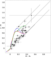 |
Fig. 1 2MASS colour-colour diagram. The red, green, and blue lines represent the main sequence, supergiant and giant locations, respectively. These were built from the PARSEC evolutionary tracks8 with Solar metallicity. The dashed grey lines are 10 mag length reddening vectors. The upward and downward triangles are the classified cool stars (#1, #9, and #30) and the suspected cool ones (#3, #4, and #7), respectively. |
6 Physical parameters
Because our goal is to determine as independently as possible the different quantities involved in the momentum balance equation which characterises SBNs, we derived the physical parameters for the stars, bow shocks, and their local environment. The SBNs and the stellar transverse velocity vectors are shown in Fig. C.1, while the physical quantities discussed below are summarised in Table A.4.
6.1 Stellar distance and transverse velocity
With regard to the distance of the star, we adopted the distance estimated from parallaxes by Bailer-Jones et al. (2021) or, if not available (as was the case for star #25), the usual spectrophotometric distance, following Russeil (2003). We then have star, and hence bow-shock, distances ranging from 555 pc to 9328 pc, with 76.6% of them between 1300 and 5000 pc. We used the proper motions and the parallaxes retrieved from Gaia EDR3 to calculate the Galactic transverse velocity components of the star with respect to the local interstellar medium, following Russeil et al. (2020). To ensure good quality of the transverse velocity vector (Vt), it was calculated only for stars with a parallax π > 0, a relative uncertainty σπ / π ≤ 0.2, and RUWE9 ≤ 1.4 (Fabricius et al. 2021).
With these constraints, we could calculate Vt for 37 of the 47 stars and find Vt between 2.9 and 120.6 km/s (median value 23 km/s). Because the radial velocity is not known for most of the stars, the transverse velocity, Vt, is then a lower limit for the true stellar velocity. However we adopt it as the space velocity of the star with respect to the ambient medium. Mackey et al. (2021), from simulations, show that the arcuate shape of the SBN is prominent only if it is seen edge-on (inclination angle greater than 45°). Since they were identified on the basis of their arcuate morphology, we can assume that the peculiar velocity is dominated by the transverse component rather than the radial one. To check this hypothesis, we considered the 20 stars for which the radial heliocentric velocity is given in the SIMBAD10 database, Gaia DR3 database, or Chick et al. (2020). After heliocentric to Local Standard of Rest (LSR) conversion, the peculiar radial velocity was calculated and quadratically added to Vt. We find that the ratio between the full space velocity and Vt is on average 1.54, with only three stars showing a ratio larger than 2 (stars #1, #33, and #36). We can then conclude that Vt is a representative measure of the stellar velocity (with respect to the ambient medium).
The assumption that bow shocks require supersonic star-ISM relative velocity suggests that runaway stars are good candidates. The velocity threshold adopted to define a runaway star depends on the authors, but also on whether the considered velocity is the full, the radial, or the transverse one. The velocity threshold is usually between 25 km/s and 40 km/s (Blaauw 1961; Tetzlaff et al. 2011; Kobulnicky & Chick 2022). Following Kobulnicky & Chick (2022), we adopted a threshold of 25 km/s and find that 17 stars (among the 37 with a determined Vt) are runaways, among which 15 are isolated. In addition, one can note that only five stars have a Vt vector pointing at more than 45° away from the Galactic plane (among which only two are runaways). This has already been observed for the morphology and kinematics position angles of previous samples of SBN central stars (Kobulnicky et al. 2016; Kobulnicky & Chick 2022). Kobulnicky & Chick (2022) explain that by a selection effect, arguing that OB stars with a velocity vector perpendicular to the Galactic plane quickly reach the less dense region of the disk, which minimises the probability of producing a detectable bow shock.
6.2 Stellar mass-loss rate
From the spectral type, we adopted the stellar temperature (Te f f) and mass from Schmidt-Kaler (1982) and de Jager & Nieuwenhuijzen (1987) for B stars and from Martins et al. (2005a) for O stars. With the AV determined in Sect. 5, we determined the Ks and G absolute magnitudes (the AV to AKs and AG conversion factors are from Wang & Chen 2019). From the MIST11 database, we evaluated (retrieving the values for solar metallicity and log g between 2 and 4.5) the bolometric corrections (BC) to apply to the Ks and G absolute magnitudes. The BC appears to mainly depend on Te f f, while the log g dependence can be taken into account as a typical uncertainty of 0.1 mag. The stellar luminosity was calculated adopting the Solar bolometric magnitude from Willmer (2018) and the values obtained from Ks and G magnitudes were averaged (if there was only one value, that was adopted). We then used relations from Vink et al. (2001) to evaluate the mass-loss rate (![Mathematical equation: $\[\dot{M}\]$](/articles/aa/full_html/2025/06/aa52262-24/aa52262-24-eq2.png) ) from the adopted luminosity, mass, and Te f f (and assuming Solar metallicity). For our sample,
) from the adopted luminosity, mass, and Te f f (and assuming Solar metallicity). For our sample, ![Mathematical equation: $\[\dot{M}\]$](/articles/aa/full_html/2025/06/aa52262-24/aa52262-24-eq3.png) is between 2 10−14 M⊙ yr−1 and 1.8 10−5 M⊙ yr−1. This is in agreement with the
is between 2 10−14 M⊙ yr−1 and 1.8 10−5 M⊙ yr−1. This is in agreement with the ![Mathematical equation: $\[\dot{M}\]$](/articles/aa/full_html/2025/06/aa52262-24/aa52262-24-eq4.png) found by Peri et al. (2012), Kobulnicky et al. (2018) and Kobulnicky et al. (2019) for other samples of SBN star candidates. We have to keep in mind that, while there is a general agreement between Vink et al. (2001) and
found by Peri et al. (2012), Kobulnicky et al. (2018) and Kobulnicky et al. (2019) for other samples of SBN star candidates. We have to keep in mind that, while there is a general agreement between Vink et al. (2001) and ![Mathematical equation: $\[\dot{M}\]$](/articles/aa/full_html/2025/06/aa52262-24/aa52262-24-eq5.png) observed by various techniques (in particular the one developed by Kobulnicky et al. 2018),
observed by various techniques (in particular the one developed by Kobulnicky et al. 2018), ![Mathematical equation: $\[\dot{M}\]$](/articles/aa/full_html/2025/06/aa52262-24/aa52262-24-eq6.png) evaluations suffer from uncertainties that impact the quantities derived in Sect. 7. For example, with an
evaluations suffer from uncertainties that impact the quantities derived in Sect. 7. For example, with an ![Mathematical equation: $\[\dot{M}\]$](/articles/aa/full_html/2025/06/aa52262-24/aa52262-24-eq7.png) on average a factor of 2.7 below the Vink et al. (2001) prescription, as Kobulnicky et al. (2019) find, we can estimate that Vt would be 60% smaller when it is calculated from Eq. (1).
on average a factor of 2.7 below the Vink et al. (2001) prescription, as Kobulnicky et al. (2019) find, we can estimate that Vt would be 60% smaller when it is calculated from Eq. (1).
6.3 Density of the local interstellar medium
Kobulnicky et al. 2018 developed a method to measure the local interstellar medium based on the infrared surface brightness of the nebula. Here we propose to estimate the ambient density in a way independent of the shock itself. For this we used the HI4PI datacubes (HI4PI Collaboration 2016). These have an angular resolution of 16.2′ and a spectral resolution of 1.28 km/s. From the adopted distance of the star, we first evaluated the VLS R (the radial velocity in the local standard of rest) of the local interstellar medium, assuming that it follows the rotation curve from Russeil et al. (2017). We then measured the column density (assuming optical thin HI emission), integrating the HI profile on a 10 km/s velocity range (characteristic velocity dispersion for the warm neutral gas in the inner Galaxy; Marasco et al. 2017) around the VLS R and in a circular aperture of 720″ radius (this size was chosen to be representative of an area of constant column density and comes from a compromise between the average size of the sources, which is 9″, the spatial resolution of the survey and the size of the background structures observed there), centred on the star position. Assuming a spherical geometry, we then deduced the HI number density (cm−3), which was expected to be an upper limit for the ambient density. We find a mean density of ⟨nup⟩ = 32.2 cm−3, which is in agreement with the average values found by Peri et al. (2012), Peri et al. (2015), and Kobulnicky et al. (2018) (a slightly larger mean value of 102 cm−3 is reported in Kobulnicky et al. 2019).
We also estimated the ambient density using the HI4PI total column density map (HI4PI Collaboration 2016), from which, following Ochsendorf et al. (2014), we evaluated the average HI density along the line of sight by dividing the total column density at the position of the star by its distance. This gives us a lower estimate for the local interstellar medium (⟨nlow⟩ = 1.9 cm−3).
Figure 2 shows that, if the two methods give different values they are, nevertheless, quite well correlated. Both methods assume a homogeneous medium but correspond to different scaling; the correlation can then suggest that most stars are in a similar environment, although density inhomogeneities are difficult to evaluate. Five stars, with nlow larger than 3 cm−3, strongly depart from the tendency. These stars are among those at the smallest Galactic longitudes (between 27° and 35°) and are less than 2 kpc away. The two stars with the highest density are also the closest ones (less than 610 pc). This shows that our approaches have significant limitations for stars that are closer than 2 kpc. Indeed, nup is badly estimated because the relationship between kinematic distance and velocity does not work for close objects, and nlow is poorly calculated for nearby stars since the background emission is likely to dominate the HI integrated emission. In Fig. 2 we also compare the different estimates to the expected relations between density and the Galactic plane distance, z (e.g. Dickey & Lockman 1990; Loup et al. 1993). Globally, nlow and nup follow the general trend expected for an exponential disk, while discrepancies can be attributed to local density increases due to star-forming regions, as illustrated by the stars in the well-known Cygnus X region and for which Emig et al. (2022) measure electron densities between 10 cm−3 and 400 cm−3.
The densities that we evaluate here using the different arc regimes presented in Fig. 2 of Henney & Arthur (2019a) (which combine the density, the ambiant velocity, and the stellar mass), suggest to us that only three stars (#5, #12, and #40) would possibly develop a radiation bow wave, instead of a wind bow shock, if nup is adopted.
6.4 Geometrical quantities
Similarly to Kobulnicky et al. (2018), we re-evaluated the standoff distance, R0, defined as the distance between the stellar candidate and the bow shock apex. It is measured directly from mid-infrared images (MIPS 24 μm, WISE 22 μm, or Herschel 70 μm). Since estimating the distance to the apex is made difficult when the star is off-centred relative to the bow geometry and/or when the bow morphology is irregular, we estimate an uncertainty of 20% on the measurement of R0. In our sample of 47 sources, we find R0 in the range 0.01–1.5 pc. We also estimate the distance from the stellar position to the bow shock at 90° (R90) of the apex direction. We find a mean R0 / R90 ratio of 0.57, in good agreement with values found by Meyer et al. (2014) for modelled bow shocks around massive runaway stars.
In addition, we measured the position angle (PA) difference between the SBN morphological axis and the Vt direction (ΔPA). We find 9 stars (of which 7 are runaways) with Vt well aligned with the SBN (ΔPA < 45°), 6 stars (of which 3 are runaways) with Vt pointing in the SBN opposite direction (ΔPA = 180° ± 45°), and 21 stars (of which 10 are runaways) in the intermediate ΔPA. So we have a majority of non-aligned cases. This is in agreement with Kobulnicky & Chick (2022) who, analysing ΔPA for a larger sample (267 SBNs), identify two populations: a small one (31% of their sample) of highly aligned (Gaussian width of 25°) and the other one with a majority of random non-aligned cases. They conclude that the local environment factors rather than the stellar motion dominate the formation of BSs.
On the other hand, from the theoretical expression of the standoff distance (recalled in Eq. (1)) it is expected that R0 ∝ Vt−1, R0 ∝ ![Mathematical equation: $\[\dot{M}\]$](/articles/aa/full_html/2025/06/aa52262-24/aa52262-24-eq8.png) 1/2, and R0 ∝ n−1/2. Plotting these quantities (Fig. 3), we find a slope (in log scale) of 0.18 (correlation coefficient r = 0.78) and −0.69 (correlation coefficient r = −0.57) for R0 versus
1/2, and R0 ∝ n−1/2. Plotting these quantities (Fig. 3), we find a slope (in log scale) of 0.18 (correlation coefficient r = 0.78) and −0.69 (correlation coefficient r = −0.57) for R0 versus ![Mathematical equation: $\[\dot{M}\]$](/articles/aa/full_html/2025/06/aa52262-24/aa52262-24-eq9.png) and nlow, respectively. Obviously, the R0 versus nlow correlation is poor and so not significant. The discrepancy with the theoretical expression is most important for R0 versus Vt, as we do not find the expected decreasing behaviour. This seems to suggest that, in most cases, the relative velocity of the ambient ISM may come more from the motion of the ISM itself than from the velocity of the star in the ISM. However, the expected velocity trend may also simply be blurred because we compared objects that have different mass-loss values and that are located in different density environments. So
and nlow, respectively. Obviously, the R0 versus nlow correlation is poor and so not significant. The discrepancy with the theoretical expression is most important for R0 versus Vt, as we do not find the expected decreasing behaviour. This seems to suggest that, in most cases, the relative velocity of the ambient ISM may come more from the motion of the ISM itself than from the velocity of the star in the ISM. However, the expected velocity trend may also simply be blurred because we compared objects that have different mass-loss values and that are located in different density environments. So ![Mathematical equation: $\[\dot{M}\]$](/articles/aa/full_html/2025/06/aa52262-24/aa52262-24-eq10.png) seems to be the main parameter that correlates with R0, as already supported by Kobulnicky et al. (2018, 2019).
seems to be the main parameter that correlates with R0, as already supported by Kobulnicky et al. (2018, 2019).
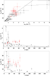 |
Fig. 2 Local ISM density evaluation in the direction of the BS. The upper plot shows nup versus nlow. The fitted dashed line follows nup = 16.8 nlow + 2.3. The middle and lower plots show nlow and nup versus the distance above the Galactic plane, z, respectively. The dashed line draws the Dickey & Lockman 1990 and Loup et al. 1993 tendencies. In all the plots, the red points are the stars in the Cygnus X region (1 ~ 79°). |
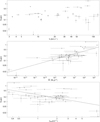 |
Fig. 3 Log–log plots of the dependencies of R0 relative to Vt (upper), mass-loss rate (middle), and nlow density (bottom). The dashed lines are the fitted tendencies. |
7 Discussion
The relative velocity between the central star and the interstellar medium is often invoked to explain the creation of an observable bow shock. As underlined by, for example, Kobulnicky & Chick (2022), for this, it is expected that this relative velocity is provided either by the supersonic motion of the star with respect to the ISM (called a runaway star) and/or a bulk ISM flow due to photoevaporative or champagne flows in H II regions. In this context, the theoretical momentum-driven SBN relation leads to the following expression for the standoff distance (e.g. Kobulnicky et al. 2010):
![Mathematical equation: $\[R_0=\sqrt{\frac{V_w \dot{M}}{4 \pi \rho_a V_a^2}},\]$](/articles/aa/full_html/2025/06/aa52262-24/aa52262-24-eq11.png) (1)
(1)
where Vw and ![Mathematical equation: $\[\dot{M}\]$](/articles/aa/full_html/2025/06/aa52262-24/aa52262-24-eq12.png) are the stellar wind velocity and mass-loss rate, respectively, and Va and ρa are the ambient relative velocity flow and local ISM density, respectively (ρa = μna, with the mean ISM gas mass per H atom μ = 2.36 × 10⁻²⁴ g, Povich et al. 2008). The adopted terminal wind velocities, Vw, were from Martins et al. (2005a), Prinja & Massa (1998), and Lamers et al. (1995) for O-, B-, and A-type stars, respectively.
are the stellar wind velocity and mass-loss rate, respectively, and Va and ρa are the ambient relative velocity flow and local ISM density, respectively (ρa = μna, with the mean ISM gas mass per H atom μ = 2.36 × 10⁻²⁴ g, Povich et al. 2008). The adopted terminal wind velocities, Vw, were from Martins et al. (2005a), Prinja & Massa (1998), and Lamers et al. (1995) for O-, B-, and A-type stars, respectively.
Adopting the established values for the mass-loss rate, wind terminal velocity, and standoff distance, this relation can be used in different ways. For stars for which we are not able to determine Vt, the relation is used to determine it from nlow and nup. For stars with Vt aligned with the SBN, then the transverse component of the ambient ISM velocity flow, Va, corresponds to Vt, and the relation can be used to re-evaluate the ambient density. For stars with Vt not aligned with the SBN apex direction, Vt is no longer representative of the relative ambient medium velocity. We then used the relation to evaluate Va and subsequently the expected ISM flow velocity, Vflow (with Vflow = Va − Vt × cos (ΔPA)). All these quantities are summarised in Table A.5.
However, other processes can also lead to the formation of bows. For example, Henney & Arthur (2019a) recall that, whereas bow shocks are usually attributed to the star’s wind – ISM interaction (wind-supported bow shocks, WBSs) there are regimes where the bows can be supported by the radiation (radiation-supported bow waves, RBWs, and radiation-supported bow shocks, RBSs). In particular, Henney & Arthur (2019b) underline that WBSs dominate for fast-moving stars and for low-density environments, RBWs are important for B stars and weak-wind O stars in moderate density environments (n > 100 cm−3), and RBSs apply to slow-moving O stars in dense environments. In bow waves, the distance (RBW) where dust grains are stopped due to radiation pressure should exceed the bow-shock standoff distance, R0. However, Ochsendorf et al. (2014) showed that for O stars earlier than O6 and early type-B supergiants, it is expected that RBW < R0, while for dwarf stars with spectral type later than O6, RBW > R0. In addition, they showed that creating dust waves is most efficient around relatively slowly moving stars. For example, Ochsendorf et al. (2014) argued that the arc structure engulfing σ Ori AB (with a space velocity of only 15.1 km/s) is a dust wave in which the radiation pressure has stalled the dust carried along by the IC 434 photoevaporative flow of ionised gas coming from the dark cloud L1630. In parallel, Ngoumou et al. (2013) observed an arc-shaped feature around a high-velocity (100 km/s) B star near the stellar cluster Trumpler 14. They noted that the star is not centred with respect to the bow, but showed that it is at the edge of a molecular clump. They then argued that the arc is a bow shock produced by the stellar wind while the star is grazing along the surface of the clump, showing, from simulation, that the non-axisymmetry of the feature is consistent with the presence of a density gradient perpendicular to the bow shock. More generally, Wilkin (2000) theoretically showed that flows at oblique angles relative to a moving star can produce asymmetric bow-shock nebulae.
In addition, as underlined by Kobulnicky & Chick (2022), since Vt is calculated assuming a circular orbit model, it does not take into account circular velocity departures due to the cloud-to-cloud velocity dispersion of the ISM and streaming motion along the arms. Indeed, arm perturbation can introduce radial and azimuthal gas streaming motions (e.g. Roberts 1969; Englmaier 2000; Ramón-Fox & Bonnell 2018) which translate into average peculiar motions towards the Galaxy centre and opposite to Galactic rotation. Such velocity departures are well known for the Perseus arm for Galactic longitudes between 90° and 160° (e.g. Roberts 1972; Brand & Blitz 1993). Typical velocity departures are about 10 km/s (e.g. Anderson et al. 2012; Wienen et al. 2015), but can reach up to 40 km/s (Brand & Blitz 1993). They can explain some of the cases of misalignment between the SBNs and Vt.
In our sample, for most of the stars, their transverse velocity is not aligned with their SBN axis. Therefore, to better understand the formation of SBNs, in the following, we study the properties of SBNs with respect to their environmental conditions.
7.1 Bow shocks in the Cygnus region
Eleven OB stars and their associated bow shocks in Cygnus X were studied by Kobulnicky et al. (2010). In this context, twelve stars (#31 to #42) of our sample can be associated with the Cygnus star-forming region, of which three (#31, #39, and #40) have already been studied by Kobulnicky et al. (2010). They classified the SBNs around these stars as ambiguous, probable, and doubtful for #31, #39, and #40, respectively, and they showed that some SBNs can be an interaction or illumination of a nearby cloud.
In our sample, the stars have distances between 1.4 and 1.9 kpc (except star #31, which has a slightly larger distance of 2.15 kpc), in agreement with the distances of the Cygnus OB associations, especially Cyg OB2 (Berlanas et al. 2019 suggest that the main Cyg OB2 association is located at a distance of 1.76 kpc, with a foreground population located around 1.35 kpc), which is the most distinct and most highly concentrated of them (Quintana & Wright 2021).
Quintana & Wright (2021) show that the Cygnus OB associations do not have the kinematic coherence expected for OB associations, leading them to identify six new OB associations (Quintana & Wright 2022), among which the C, E (Cyg OB2), and D associations (see Fig. 1 in Quintana & Wright 2022) show clearly different motions. Indeed, associations D and E move in the direction of increasing Galactic coordinates, while C moves in the opposite direction. In this context, we note that three stars (#37, #40, and #42) are moving in the direction of increasing Galactic coordinates, while six stars (#33, #34, #35, #36, #39, and #41) are moving in the opposite direction, consistent with these stellar association motions.
As already noted by Kobulnicky et al. (2010), the orientation of the SBNs and of Vt appear random and have no preferential alignment with respect to Cyg OB2, as expected if the stars are runaways originating from this association or if Cyg OB2 is at the origin of the local ISM pressure. Except for star #31, which is a runaway, the others have Vt between 3.4 and 13.4 km/s, more representative of the motion of the stars within their parent association (Ward & Kruijssen 2018 measure stellar velocity dispersion in associations between 3 and 13 km/s).
Runaway star #31 has its Vt vector pointing back to Cyg OB2. Taking into account its velocity and its angular distance to Cygnus OB2 (~3.2°), we estimate a travel time to its current position of 2.4 Myr, in agreement with the typical age of ~2.5 Myr for Cygnus OB2 (Negueruela et al. 2008). It is, therefore, very likely that this star originates from Cygnus OB2.
Because none of the other stars are runaways (although stars #33 and #36 seem to be runaways when considering their 3D velocity), the bows should be formed due to a bulk ISM flow, as is also supported by the non-isolated status assigned for nine of them by Jayasinghe et al. (2019). The ISM in the Cygnus region is very filamentary and Emig et al. (2022) measure electron densities of the filamentary structures between 10 cm−3 and 400 cm−3 (with a median value of 35 cm−3). For three of the four aligned objects (#31, #39, and #40), the density evaluated from Eq. 1 is in this range, while for #41 (a B6.5I) a much lower density (410−3 cm−3) is required to account for the measured R0. However, #41 is quite unusual, as its SBN is better seen at Herschel-70 μm and WISE-12 μm than at WISE-22 μm which, in addition to the extremely low density estimated, means its nature is still to be clarified. For the two objects (#32 and #38) with no Vt, the estimated velocity is between 2 and 40 km/s. However, for #38 the SBN seems doubtful as the star is not centred on the arc and the bow follows a larger-scale feature.
Lastly, concerning the six non-aligned objects (stars #33 to #37 and #42), for four of them (#34 to #37), depending on the density, an estimated Vflow in agreement with the typical ISM velocity (which is between ~6 km/s for typical photoevaporative outflow velocity, e.g. McLeod et al. 2015, and 30 km/s for gas velocity in the Champagne phase H II region, e.g. Tenorio-Tagle 1979) is found. Such photoevaporative flows could be invoked to explain the SBNs for stars #34 to #36, as they are less than 4′ (~1.6 pc) away from a bright rim and in the direction in which their bow points. For star #33, the estimated Vflow is very large (45 or 153 km/s for nup and nlow, respectively) and no origin for this flow is identifiable. One could assume that, as this star is a runaway, thanks to its radial velocity component, the direction of the bow could be due to density gradient.
7.2 Bow shocks in H II regions
In RCW 49 and M17, Povich et al. (2008) detected SBNs pointing towards the exciting clusters around OB stars located in the PDR and at the periphery of the cluster, providing very obvious examples of SBNs in H II regions. In addition, 24 μm emission is frequently observed within H II regions and near the exciting stars (e.g. Deharveng et al. 2010), occasionally exhibiting an arcuate shape, as seen in RCW 82 (Pomarès et al. 2009) and RCW 120 (Zavagno et al. 2007).
Five stars in our sample are associated with H II regions. Stars #6 and #44 are found inside the optical H II regions Sh2-66 and Sh2-135, respectively. While stars #12 and #29 are situated on the edge of radio H II regions catalogued as GB6J1910+0814 and GB6J1952+2610 (also identified as the IR bubble N131 by Churchwell et al. 2006), respectively, by Gregory et al. (1996), star #23 appears to be located at the edge of the optical H II region Sh2-86.
Star #44, at a projected distance of 2.5 pc from the main pillar’s tip (Fig. 4 – upper panel) is the main ionising source of the H II region Sh2-135 (Lahulla 1985) and shows its SBN facing a very bright rim with pillars. The density calculated from Eq. 1 (Table A.5) is around 283 cm−3 larger than nup. However, from the radio flux (given by Anderson et al. 2016), we estimate (using Eq. (4) in Das et al. 2018) an electron density of ~39 cm−3. Adopting this last value, a Vflow of 16 km/s is then required to find the measured R0. Since Pismis et al. (1986) reported that Sh2-135 is a blister-like H II region with the ionising gas flowing away from the CO cloud with a line of sight velocity of 4 km/s, the SBN could be produced by a photoevaporative flow coming from the rim.
Star #6 is located in Sh2-66 and has its SBN facing a dark cloud (Fig. 4 – lower panel). Because of a bad RUWE, Vt is not estimated and the parallactic distance (8.6 kpc) is very uncertain. This distance is very different from the spectrophotometric distance (3.6 kpc, Forbes 1989) and favours the far kinematic distance (near and far distances are 2.9 or 11.4 kpc, respectively, calculated from the Fich et al. 1990 Hα LSR velocity of 46.8 km/s for the H II region). The star is at the centre of the region and is probably the main exciting source, while its projected distance to the dark cloud is ~4.2 pc (for a distance of 8.6 kpc). From the radio flux (given by Anderson et al. 2015), we estimate an electron density of ~25.5 cm−3, in agreement with nup. Due to its similar velocity (VLS R = 44.9 km/s, Eden et al. 2012), the dark cloud (GRS G030.44 +00.44) can be linked to the H II region. The PDR and the dark cloud are barely distinguishable from the background in the near-IR and mid-IR wavelengths. This suggests that the H II region evolutionary state is rather advanced. The calculated Va ~ 48 km/s is quite large to be due to a photoevaporative flow alone and so better suggests the star to be a runaway.
The SBN of star #12 looks more like an enhancement in the radio H II region GB6 B1907+0809, classified as a diffuse H II region by Lockman et al. (1996). With an LSR velocity of 62 km/s (Rigby et al. 2019), the region’s near and far kinematic distances are 4.1 or 8.2 kpc, respectively. The distance of #12 is ~555 pc, making it a foreground star. In addition, it is an A5Ib star that cannot ionise the H II region.
Star #29 appears located on the edge of the IR bubble N131 (Churchwell et al. 2006). The bubble morphology suggests that this could be the PDR of an H II region that is not optically visible (Fig. C.2) and whose ionising source is unknown. According to Hou & Gao 2014 and Zhang et al. 2016, N131 is approximately 8.5 kpc away, while #29 is only 4 kpc away. The large Vt (55.3 km/s) suggests that the star is a runaway and, because the SBN and the Vt are well aligned and point outwards from the centre of the bubble, one can suspect at first glance that it has travelled from the centre of the bubble (at 5.7’). But, in this context, its travel time would be too short (0.25 Myr) with respect to the typical age for such a star (between 3.5 and 13 Myr, McEvoy et al. 2015). One can conclude that the star and its SBN are probably seen by chance in the direction of the edge of N131.
Star #23 is on the border of the optical H II region Sh2-86 (Fig. C.3). The SBN points towards the exciting cluster NGC 6823 and the distance of #23 is in agreement with that of NGC 6823 (2 kpc, e.g. Riaz et al. 2012). Located in an optically dark filament identified as a molecular filament by Kohno et al. (2022), we favour nup and then estimate a low velocity (Vt ~ 7.7 km/s) for the star. However, the nature of the SBN must be made clear, as it is straight rather than arched, and seems to be connected to a larger scale extension.
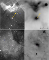 |
Fig. 4 IPHAS-Hα (left) and MIPS 24 μm (right) images of Sh2-135 (upper panel) and Sh2-66 (lower panel). In the upper panel, the arrow is the transverse velocity vector (arbitrary length) for star #44. In the lower panel, star #6 is indicated by the cross. The images are oriented according to Galactic coordinates. |
7.3 Bow shock in the cluster Berkeley 97
Star #46 (HD 240016) is observed in the direction of the open cluster Berkeley 97. The distance for Berkeley 97 is 1.8 kpc (Tadross 2008), 2.5 kpc (Dias et al. 2021), or 3.2 kpc (Poggio et al. 2021). Covered only by WISE (low spatial resolution), about 16 stars belonging to Berkeley 97 (Hunt & Reffert 2023) are observed in the SBN footprint. Among them is the star HD 240015, separated by 50.6" from #46. HD 240015 has a similar magnitude to #46 and is classified as a B0.5II star by Dinçel et al. (2024). Both stars have similar distances (Bailer-Jones et al. 2021); so, as in Dinçel et al. (2024), we can assume that #46 also belongs to the cluster and then that they are the two most massive stars of the cluster. This cluster, with log(age[yr]) ~ 7.1 (Dinçel et al. 2024), does not show an H II region and seems to be in a cleared environment, suggesting that nlow is to be favoured. This is in agreement with recent results from Dinçel et al. (2024), who show that the cluster is surrounded by an H I void.
For #46 (poor RUWE value), Vt cannot be evaluated; nonetheless, its radial velocity (~32 km/s) indicates that it is a runaway, even though its motion may be severely influenced by binarity and internal motion in the cluster. The nature of the SBN is not clear either, because the cluster seems to move in the opposite direction and no interstellar medium is noted close to it.
In this context, and because #46 is not centred relative to the SBN, the SBN could be due either to a joint contribution from #46 and HD 240015 or due to the combined and unresolved contribution of the stars observed in the SBN footprint. Another alternative could be that the mid-IR emission comes from the wind interaction with any supernovae remnant as, given the age of the cluster, the most massive stars should have become supernovae. This scenario would be in agreement with Dinçel et al. (2024), who speculate that the H I void could underline a dissipated supernova remnant (SNR) and that some part of the dust dragged inward by the reverse shock interacts with massive stars to form the observed SBN. Higher spatial resolution analysis of the SBN is then needed to clarify its nature.
7.4 Bow shocks around cool stars
Scherer et al. (2020) point out that cool stars drive supersonic winds and may show bow shocks if the star has velocity with respect to the ambient ISM. In parallel, Cox et al. (2012) pointed out that evolved stars lose material, via a dusty wind, during their asymptotic giant branch (AGB) and supergiant phase, developing extended envelopes which can then form bow shocks, as around Betelgeuse which is the best example of such phenomenon (Mohamed et al. 2012).
Here, the spectral classification suggests that stars #1, #9, and #30 are cool stars, while all of them display a Vt that is not aligned with the SBN. For #1 and #9, the SBN is thick, with an irregular shape and a thin surrounding secondary arc (better seen at IRAC-8 μm), suggesting that it could better underline a photodissociation region. In addition, their SBNs present radio counterparts (HRDSG027.334+00.176 and HRDSG034.031-00.59 for #1 and #9, respectively) classified as H II regions by Anderson et al. (2011). From the main radio recombination line velocity measured by Anderson et al. (2011), HRDSG027.334+00.176 and HRDSG034.031-00.59 would be at the near kinematic distances of 4.6 and 3.4 kpc, respectively. With a distance of 1.06 and 1.65 kpc, respectively, #1 and #9 then seem to be foreground stars, not related to the background H II regions. For star #30, because it is not centred relative to the SBN and its Vt is not aligned with the SBN, one suspects that it is probably not the SBN driver. Based solely on an adequate direction and value of their tangential velocities, the 2MASS sources 19533053+2808202 or 19533020+2808216 would be better candidates.
Possible parent cluster.
7.5 Bow shocks of velocity aligned stars
In addition to the stars in the Cygnus region and H II regions, we have four star candidates with ΔPA < 45° and four others with 45° < ΔPA < 52° (see Table A.4). One can consider here that they have their Vt and their SBN aligned. These are #5, #10, #11, #13, #14, #16, #43, and #47. Among them, #13, #14, #16, #43, and #47 are runaways (Vt> 25 km/s). One notes also that, except for star #10 (n ~ 34 cm−3), their measured parameters suggest a low density (between 0.003 and 3.4 cm−3), in agreement with the weakly structured local environment aspect seen on the Spitzer 8 μm and mid-IR images, WISE 22 μm, and/or Spitzer 24 μm images (Fig. C.1).
There are two main scenarios to explain the presence of runaway or walkaway stars (stars with velocities of 5–30 km/s, de Mink et al. 2014): the binary supernova scenario (Blaauw 1961; Hoogerwerf et al. 2001) and the dynamical ejection from star clusters scenario (e.g. Hoogerwerf et al. 2001; Fujii & Portegies Zwart 2011). We then searched the possible origin for these stars by simply looking for clusters (with similar distances to the stars) present on the straight line drawn backwards. For that we used the stellar cluster catalogues from Hunt & Reffert (2023), Just et al. (2023), and Cantat-Gaudin et al. (2020). Table 1 summarises our findings, where β is the angular separation distance between the SBN and the candidate parental cluster from which the travel time (noted Tt) is calculated.
Star #5 has a low velocity (Vt = 8.22 km/s) and is identified as a member of the cluster Theia 12 (Kounkel & Covey 2019) by Hunt & Reffert (2023). It is located at the periphery of the cluster, which has a radius of 2.5° (Hunt & Reffert 2023). Due to the large extension of the cluster, it is difficult to know if the star is being ejected from the cluster or if its velocity is only representative of its motion in the cluster.
For most of the other stars we can find a possible parental cluster. Assuming that the star has been ejected early, the flight time, Tt, is expected to represent the star’s age. We find that Tt is between 1.62 and 4.54 Myr, in agreement with the typical age of O- and B-type stars (e.g. Weidner & Vink 2010; Daszyńska-Daszkiewicz & Miszuda 2019). For star #13, two clusters, MWSC 3093 and MWSC 3096 (Kharchenko et al. 2016), in the extreme star-forming complex W51, could be the ones it originates from. For this star, the cluster age and Tt are in agreement with the dynamical ejection scenario. For stars #11, #14, #16, #43, and #47 the cluster age is roughly two orders of magnitude larger than Tt. These stars could have been ejected later after their formation via the binary supernova process, since the age of the clusters suggests that the most massive stars should have already exploded into supernovae (e.g. Crowther 2012, Eldridge & Stanway 2022). Finally, for star #10, no parental cluster candidate is found. This star is moving in the direction of the Galactic plane and is located in an elongated structure (possibly a cloud) visible from 8 μm to 250 μm. This could explain the higher density of its surrounding ISM, which would favour SBN formation.
7.6 Other bow shocks
There remain 18 stars, of which five have no calculated Vt, while the others have ΔPA > 52°.
Among them, stars #3, #4, and #7 have no spectral type, and then no characteristic can be established.
For the five stars with no Vt (#18, #25, #26, #28, and #45) we estimate the expected velocity needed to produce the SBN. Depending on the density, these stars can be runaways or not, except for #45 which, whatever the density, has a low velocity and #26, which shows an unrealistic velocity (larger than 200 km/s). For #18, because of its large Galactic plane distance of 168.9 pc, we would favour nlow, hence a runaway status with a velocity of 86.5 km/s.
For the other thirteen stars with misaligned Vt (#2, #3, #4, #7, #8, #15, #17, #19, #20, #21, #22, #24, and #27), eight of them (#2, #4, #15, #17, #19, #20, #21, and #22) are runaways (with Vt between 31.3 and 80.7 km/s), for which it is therefore difficult to understand the misalignment of their bow shock relative to their transverse velocity direction. For #20, the suggested Vflow is unrealistic (>100 km/s), but its SBN clearly points towards the star-forming region GAL54.4+01 (Day et al. 1972) (which is at a similar distance of 7.3 ± 1 kpc, Anderson et al. 2012), while its Vt direction suggests it could have been ejected from it.
Five stars (#24, #25, #26, #27, and #28) are observed in the Vulpecula OB1 association region, which is a region of active star formation (Billot et al. 2010). Three of them (#26, #27, and #28) have their SBNs facing Sh2-87 (distance ~ 2.3 kpc; Xue & Wu 2008), while the others (#24 and #25) have their SBNs pointing towards pillars which themselves point in the opposite direction towards stars belonging to the Vulpecula OB1 association (distance ~ 1.6 kpc; Mel’nik & Dambis 2017). But #25, #26, and #28 have a distance placing them farther away, and so not related to these structures. Conversely, stars #24 and #27, due to their distance (~2 kpc) and their Vt < 20 km/s, may belong to the Vulpecula OB1 association.
Six stars exhibit a SBN with a remarkable morphology (see Fig. C.1): #2 shows two cirrus-like arcs on either side of the star, #7 has a quasi-circular aspect (it is also classified as a bubble MWP1G031117+007214 by Simpson et al. 2012), #17 is surrounded by irregular structures of the ISM, #22 has an isolated long, thin and distorted SBN (it shows the largest R0 ~ 1.5 pc), #26 has four small radial finger-shaped extensions which extend from the SBN, one of which passes through the star, and #28 has an SBN drawing three parallel arcs. Several explanations can be invoked to explain these shapes: the SBN may be formed by a density gradient perpendicular to the Vt (e.g. Ngoumou et al. 2013), or it is a simple enhancement of the local interstellar medium, or it is due to previous stellar mass ejections (#26 and #28 are long-period variable candidates from Lebzelter et al. 2023), or it is caused by dust grains interacting with the interstellar magnetic field while disturbed by the stellar wind collision (e.g. Katushkina et al. 2018).
Three stars are found in the direction of SNRs: #17, #21, and #22 fall in the direction of the SNRs G53.4+0.03 (Anderson et al. 2017), G55.0+0.3 (Green et al. 2022), and G56.56-0.75 (Anderson et al. 2017), respectively. The SNR-SBN link is difficult to establish because the SNR’s distance is not well constrained. In addition, their SBNs do not point towards the SNR’s centre, making their link uncertain. Furthermore, their stellar Vt does not point away from the SNR’s centre, indicating that these stars were not expelled during the supernova explosion. In this context, at least for #17, the SBN could simply be an ISM substructure shaped by the SNR.
8 Conclusions and perspectives
We led a 400–800 nm spectral survey of a sample of 47 candidate bow-shock stars. We complemented these observations with Gaia ERD3 data to find their transverse velocity relative to the interstellar medium. We find that, of the 47 candidates, there are 3 unclassifiable stars, 3 cool stars, 2 A-type stars, 10 O stars, and 29 B (mainly giant and supergiant) stars. We find that 17 stars (among the 37 with determined Vt) are runaways, of which 15 are isolated, but only 7 have their transverse velocity aligned with the SBN axis. This confirms that runaway is not the only origin for SBN formation.
We estimated, as independently as possible, the different quantities involved in the momentum balance equation which characterises the SBN. The uncertainties are large and only the relationship between R0 and ![Mathematical equation: $\[\dot{M}\]$](/articles/aa/full_html/2025/06/aa52262-24/aa52262-24-eq13.png) seems robust, confirming that the stellar wind is the most important parameter. The misalignment between the SBN axis and the transverse velocity direction of the star is observed even for runaway stars, suggesting that the environment (ambient density inhomogeneity, ISM flows, etc.) has a strong influence on the appearance and asymmetry of the bow shocks.
seems robust, confirming that the stellar wind is the most important parameter. The misalignment between the SBN axis and the transverse velocity direction of the star is observed even for runaway stars, suggesting that the environment (ambient density inhomogeneity, ISM flows, etc.) has a strong influence on the appearance and asymmetry of the bow shocks.
In this context, we note the diversity of environments where SBNs are observed: stellar associations, clusters, H II regions, and possibly SNRs. For stars with transverse velocity aligned with the BS, whether or not they are runaways, we were able, for most of them, to identify a possible parental cluster and we confirm that these stars are mainly located in a low-density medium. As already observed, numerous SBNs are present in the Cygnus OB stellar association, suggesting that the ISM conditions in such regions favour SBN observability. Few SBNs are observed in H II regions. For one of them (Sh2-135), the SBN could be explained by a ~16 km/s photoevaporated flow coming from the H II region molecular cloud’s interface. It appears then that it is necessary to specify the conditions for a flow to form an SBN: flow velocity and density, star distance from the interface, and so on. To validate the photoevaporative flow mechanism in SBN creation, statistical analysis of SBNs in H II regions and direct flow velocity determination are necessary. A more general approach would be to quantify and identify what causes the emergence of SBNs in star-forming regions: turbulence, magnetic field, density fluctuations, medium nature, and so on.
Finally, if few SBNs are observed in the direction of cool stars they seem to not be related.
A direct improvement of our study would be to have higher mid-resolution images for objects with only WISE-22 μm observations and to update and specify the transverse velocity value and direction through future GAIA releases.
Acknowledgements
The authors thank the anonymous refree for its his/her insightful remarks and comments. The authors acknowledge Interstellar Institute’s program “II6” and the Paris-Saclay University’s Institut Pascal for hosting discussions that nourished the development of the ideas behind this work. In particular, the authors thank P. Lesaffre for discussions during II6 and M. Dennefeld for his contribution to the observations. Based on observations made at Observatoire de Haute Provence (CNRS), France, with MISTRAL on the T193 telescope. This research also has made use of the MISTRAL database, operated at CeSAM (LAM), Marseille, France. AZ thanks the support of the Institut Universitaire de France. This research has made use of the SIMBAD database, operated at CDS, Strasbourg, France and “Aladin sky atlas” developed at CDS, Strasbourg Observatory, France.
Appendix A Tables
B-type star classification test.
O-type star classification test.
Equivalent Widths and Spectral classifcation of the stellar sample.
Adopted and measured physical quantities
Calculated quantities.
Appendix B Figures of the stellar SED
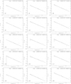 |
Fig. B.1 Spectral energy distribution (SED) of the SBN star candidates classified as OB stars. The log of the power law Fν ∝ νβ fit is shown and the slope which is the β value (and its uncertainty) is given at the top of the panels. |
Appendix C SBN images with transverse velocity vectors and additionnal figures
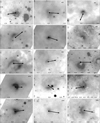 |
Fig. C.1 WISE 22μm or Spitzer-MIPS 24μm images of the studied SBN. The candidate star position and the transverse velocity vector (arbitrary length) are shown as circles and arrows, respectively. The coordinates around the frames are the Galactic coordinates (in degrees). |
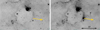 |
Fig. C.2 IRAC-8μm (left) and MIPS 24μm (right) images of N131. The displayed arrow is the transverse velocity vector (arbitrary length) for star #29. The images are oriented according to Galactic coordinates. |
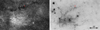 |
Fig. C.3 DSS-Red (left) and MIPS 24μm (right) images of Sh2-86. The star #6 is indicated by the cross. The images are oriented according to Galactic coordinates. |
References
- Anderson, L. D., Bania, T. M., Balser, D. S., & Rood, R. T. 2011, ApJS, 194, 32 [NASA ADS] [CrossRef] [Google Scholar]
- Anderson, L. D., Bania, T. M., Balser, D. S., & Rood, R. T. 2012, ApJ, 754, 62 [NASA ADS] [CrossRef] [Google Scholar]
- Anderson, L. D., Armentrout, W. P., Johnstone, B. M., et al. 2015, ApJS, 221, 26 [NASA ADS] [CrossRef] [Google Scholar]
- Anderson, L. D., Armentrout, W. P., Johnstone, B. M., et al. 2016, VizieR Online Data Catalog: Radio observations of Galactic WISE HII regions (Anderson+, 2015), VizieR On-line Data Catalog: J/ApJS/221/26. Originally published in: 2015ApJS..221...26A [Google Scholar]
- Anderson, L. D., Wang, Y., Bihr, S., et al. 2017, A&A, 605, A58 [NASA ADS] [CrossRef] [EDP Sciences] [Google Scholar]
- Bailer-Jones, C. A. L., Rybizki, J., Fouesneau, M., Demleitner, M., & Andrae, R. 2021, AJ, 161, 147 [Google Scholar]
- Berlanas, S. R., Herrero, A., Comerón, F., et al. 2018, A&A, 612, A50 [NASA ADS] [CrossRef] [EDP Sciences] [Google Scholar]
- Berlanas, S. R., Wright, N. J., Herrero, A., Drew, J. E., & Lennon, D. J. 2019, MNRAS, 484, 1838 [NASA ADS] [Google Scholar]
- Berlanas, S. R., Herrero, A., Comerón, F., et al. 2020, A&A, 642, A168 [NASA ADS] [CrossRef] [EDP Sciences] [Google Scholar]
- Billot, N., Noriega-Crespo, A., Carey, S., et al. 2010, ApJ, 712, 797 [NASA ADS] [CrossRef] [Google Scholar]
- Blaauw, A. 1961, Bull. Astron. Inst. Netherlands, 15, 265 [NASA ADS] [Google Scholar]
- Brand, J., & Blitz, L. 1993, A&A, 275, 67 [NASA ADS] [Google Scholar]
- Cantat-Gaudin, T., Anders, F., Castro-Ginard, A., et al. 2020, A&A, 640, A1 [NASA ADS] [CrossRef] [EDP Sciences] [Google Scholar]
- Carey, S. J., Noriega-Crespo, A., Mizuno, D. R., et al. 2009, PASP, 121, 76 [Google Scholar]
- Chambers, K. C., Magnier, E. A., Metcalfe, N., et al. 2016, arXiv e-prints [arXiv:1612.05560] [Google Scholar]
- Chick, W. T., Kobulnicky, H. A., Schurhammer, D. P., et al. 2020, ApJS, 251, 29 [NASA ADS] [CrossRef] [Google Scholar]
- Churchwell, E., Povich, M. S., Allen, D., et al. 2006, ApJ, 649, 759 [CrossRef] [Google Scholar]
- Churchwell, E., Babler, B. L., Meade, M. R., et al. 2009, PASP, 121, 213 [Google Scholar]
- Comerón, F., & Pasquali, A. 2012, A&A, 543, A101 [NASA ADS] [CrossRef] [EDP Sciences] [Google Scholar]
- Conti, P. S. 1974, ApJ, 187, 539 [Google Scholar]
- Cox, N. L. J., Kerschbaum, F., van Marle, A. J., et al. 2012, A&A, 537, A35 [NASA ADS] [CrossRef] [EDP Sciences] [Google Scholar]
- Crowther, P. 2012, Astron. Geophys., 53, 4.30 [NASA ADS] [CrossRef] [Google Scholar]
- Cutri, R. M., Skrutskie, M. F., van Dyk, S., et al. 2003, VizieR Online Data Catalog: II/246 [Google Scholar]
- Cutri, R. M., Wright, E. L., Conrow, T., et al. 2013, Explanatory Supplement to the AllWISE Data Release Products [Google Scholar]
- Das, S. R., Tej, A., Vig, S., et al. 2018, A&A, 612, A36 [NASA ADS] [CrossRef] [EDP Sciences] [Google Scholar]
- Daszyńska-Daszkiewicz, J., & Miszuda, A. 2019, ApJ, 886, 35 [Google Scholar]
- Day, G. A., Caswell, J. L., & Cooke, D. J. 1972, Aust. J. Phys. Astrophys. Suppl., 25, 1 [NASA ADS] [Google Scholar]
- Deharveng, L., Schuller, F., Anderson, L. D., et al. 2010, A&A, 523, A6 [NASA ADS] [CrossRef] [EDP Sciences] [Google Scholar]
- de Jager, C., & Nieuwenhuijzen, H. 1987, A&A, 177, 217 [NASA ADS] [Google Scholar]
- de Mink, S. E., Sana, H., Langer, N., Izzard, R. G., & Schneider, F. R. N. 2014, ApJ, 782, 7 [Google Scholar]
- Deng, D., Sun, Y., Wang, T., Wang, Y., & Jiang, B. 2022, ApJ, 935, 175 [NASA ADS] [CrossRef] [Google Scholar]
- Dias, W. S., Monteiro, H., Moitinho, A., et al. 2021, MNRAS, 504, 356 [NASA ADS] [CrossRef] [Google Scholar]
- Dickey, J. M., & Lockman, F. J. 1990, ARA&A, 28, 215 [Google Scholar]
- Didelon, P. 1982, A&AS, 50, 199 [NASA ADS] [Google Scholar]
- Dinçel, B., Sheth, S., Specht, L., et al. 2024, A&A, 691, A63 [NASA ADS] [CrossRef] [EDP Sciences] [Google Scholar]
- Drew, J. E., Greimel, R., Irwin, M. J., et al. 2005, MNRAS, 362, 753 [NASA ADS] [CrossRef] [Google Scholar]
- Eden, D. J., Moore, T. J. T., Plume, R., & Morgan, L. K. 2012, MNRAS, 422, 3178 [NASA ADS] [CrossRef] [Google Scholar]
- Eldridge, J. J., & Stanway, E. R. 2022, ARA&A, 60, 455 [NASA ADS] [CrossRef] [Google Scholar]
- Emig, K. L., White, G. J., Salas, P., et al. 2022, A&A, 664, A88 [NASA ADS] [CrossRef] [EDP Sciences] [Google Scholar]
- Englmaier, P. 2000, Rev. Mod. Astron., 13, 97 [Google Scholar]
- Evans, C. J., Howarth, I. D., Irwin, M. J., Burnley, A. W., & Harries, T. J. 2004, MNRAS, 353, 601 [NASA ADS] [CrossRef] [Google Scholar]
- Fabricius, C., Luri, X., Arenou, F., et al. 2021, A&A, 649, A5 [NASA ADS] [CrossRef] [EDP Sciences] [Google Scholar]
- Fich, M., Treffers, R. R., & Dahl, G. P. 1990, AJ, 99, 622 [NASA ADS] [CrossRef] [Google Scholar]
- Forbes, D. 1989, A&AS, 77, 439 [Google Scholar]
- Fujii, M. S., & Portegies Zwart, S. 2011, Science, 334, 1380 [Google Scholar]
- Gaia Collaboration (Brown, A. G. A., et al.) 2021, A&A, 649, A1 [NASA ADS] [CrossRef] [EDP Sciences] [Google Scholar]
- Georgelin, Y. M., Georgelin, Y. P., & Roux, S. 1973, A&A, 25, 337 [NASA ADS] [Google Scholar]
- Gray, R. O., & Corbally, C. J. 2009, Stellar Spectral Classification (Princeton University Press) [Google Scholar]
- Green, S., Mackey, J., Kavanagh, P., et al. 2022, A&A, 665, A35 [NASA ADS] [CrossRef] [EDP Sciences] [Google Scholar]
- Gregory, P. C., Scott, W. K., Douglas, K., & Condon, J. J. 1996, ApJS, 103, 427 [NASA ADS] [CrossRef] [Google Scholar]
- Groot, P. J., Verbeek, K., Greimel, R., et al. 2009, MNRAS, 399, 323 [NASA ADS] [CrossRef] [Google Scholar]
- Gutermuth, R. A., & Heyer, M. 2015, AJ, 149, 64 [Google Scholar]
- Gvaramadze, V. V., Kniazev, A. Y., Kroupa, P., & Oh, S. 2011, A&A, 535, A29 [NASA ADS] [CrossRef] [EDP Sciences] [Google Scholar]
- Hardorp, J., Theile, I., & Voigt, H. H. 1964, Hamburger Sternw. Warner & Swasey Obs., C03, 0 [Google Scholar]
- Henney, W. J., & Arthur, S. J. 2019a, MNRAS, 486, 3423 [NASA ADS] [CrossRef] [Google Scholar]
- Henney, W. J., & Arthur, S. J. 2019b, MNRAS, 486, 4423 [Google Scholar]
- HI4PI Collaboration (Ben Bekhti, N., et al.) 2016, A&A, 594, A116 [NASA ADS] [CrossRef] [EDP Sciences] [Google Scholar]
- Hoogerwerf, R., de Bruijne, J. H. J., & de Zeeuw, P. T. 2001, A&A, 365, 49 [NASA ADS] [CrossRef] [EDP Sciences] [Google Scholar]
- Hou, L. G., & Gao, X. Y. 2014, MNRAS, 438, 426 [Google Scholar]
- Hovhannessian, R. K., & Hovhannessian, E. R. 2001, Astrophysics, 44, 454 [Google Scholar]
- Hunt, E. L., & Reffert, S. 2023, A&A, 673, A114 [NASA ADS] [CrossRef] [EDP Sciences] [Google Scholar]
- Jaschek, M., Andrillat, Y., Houziaux, L., & Jaschek, C. 1994, A&A, 282, 911 [Google Scholar]
- Jayasinghe, T., Dixon, D., Povich, M. S., et al. 2019, MNRAS, 488, 1141 [NASA ADS] [CrossRef] [Google Scholar]
- Just, A., Piskunov, A. E., Klos, J. H., Kovaleva, D. A., & Polyachenko, E. V. 2023, A&A, 672, A187 [NASA ADS] [CrossRef] [EDP Sciences] [Google Scholar]
- Katushkina, O. A., Alexashov, D. B., Gvaramadze, V. V., & Izmodenov, V. V. 2018, MNRAS, 473, 1576 [NASA ADS] [Google Scholar]
- Kharchenko, N. V., Piskunov, A. E., Schilbach, E., Röser, S., & Scholz, R. D. 2016, A&A, 585, A101 [NASA ADS] [CrossRef] [EDP Sciences] [Google Scholar]
- Kobulnicky, H. A., & Chick, W. T. 2022, AJ, 164, 86 [CrossRef] [Google Scholar]
- Kobulnicky, H. A., Gilbert, I. J., & Kiminki, D. C. 2010, ApJ, 710, 549 [NASA ADS] [CrossRef] [Google Scholar]
- Kobulnicky, H. A., Lundquist, M. J., Bhattacharjee, A., & Kerton, C. R. 2012, AJ, 143, 71 [Google Scholar]
- Kobulnicky, H. A., Chick, W. T., Schurhammer, D. P., et al. 2016, ApJS, 227, 18 [Google Scholar]
- Kobulnicky, H. A., Chick, W. T., & Povich, M. S. 2018, ApJ, 856, 74 [Google Scholar]
- Kobulnicky, H. A., Chick, W. T., & Povich, M. S. 2019, AJ, 158, 73 [NASA ADS] [CrossRef] [Google Scholar]
- Kohno, M., Nishimura, A., Fujita, S., et al. 2022, PASJ, 74, 24 [NASA ADS] [CrossRef] [Google Scholar]
- Kounkel, M., & Covey, K. 2019, AJ, 158, 122 [Google Scholar]
- Lahulla, J. F. 1985, A&AS, 61, 537 [NASA ADS] [Google Scholar]
- Lam, M. C., Smith, R. J., Arcavi, I., et al. 2023, AJ, 166, 13 [NASA ADS] [CrossRef] [Google Scholar]
- Lamers, H. J. G. L. M., Snow, T. P., & Lindholm, D. M. 1995, ApJ, 455, 269 [Google Scholar]
- Lebzelter, T., Mowlavi, N., Lecoeur-Taibi, I., et al. 2023, A&A, 674, A15 [NASA ADS] [CrossRef] [EDP Sciences] [Google Scholar]
- Lennon, D. J., Dufton, P. L., & Fitzsimmons, A. 1993, A&AS, 97, 559 [NASA ADS] [Google Scholar]
- Leone, F., & Lanzafame, A. C. 1998, A&A, 330, 306 [NASA ADS] [Google Scholar]
- Lockman, F. J., Pisano, D. J., & Howard, G. J. 1996, ApJ, 472, 173 [Google Scholar]
- Loup, C., Forveille, T., Omont, A., & Paul, J. F. 1993, A&AS, 99, 291 [NASA ADS] [Google Scholar]
- Mackey, J., Green, S., Moutzouri, M., et al. 2021, MNRAS, 504, 983 [NASA ADS] [CrossRef] [Google Scholar]
- Maíz Apellániz, J., Sota, A., Arias, J. I., et al. 2016, ApJS, 224, 4 [CrossRef] [Google Scholar]
- Marasco, A., Fraternali, F., van der Hulst, J. M., & Oosterloo, T. 2017, A&A, 607, A106 [NASA ADS] [CrossRef] [EDP Sciences] [Google Scholar]
- Marcolino, W. L. F., Bouret, J. C., Martins, F., et al. 2009, A&A, 498, 837 [NASA ADS] [CrossRef] [EDP Sciences] [Google Scholar]
- Martinez, J. R., del Palacio, S., & Bosch-Ramon, V. 2023, A&A, 680, A99 [NASA ADS] [CrossRef] [EDP Sciences] [Google Scholar]
- Martins, F. 2018, A&A, 616, A135 [NASA ADS] [CrossRef] [EDP Sciences] [Google Scholar]
- Martins, F., & Palacios, A. 2021, A&A, 645, A67 [EDP Sciences] [Google Scholar]
- Martins, F., Schaerer, D., & Hillier, D. J. 2005a, A&A, 436, 1049 [NASA ADS] [CrossRef] [EDP Sciences] [Google Scholar]
- Martins, L. P., González Delgado, R. M., Leitherer, C., Cerviño, M., & Hauschildt, P. 2005b, MNRAS, 358, 49 [Google Scholar]
- McEvoy, C. M., Dufton, P. L., Evans, C. J., et al. 2015, A&A, 575, A70 [NASA ADS] [CrossRef] [EDP Sciences] [Google Scholar]
- McLeod, A. F., Dale, J. E., Ginsburg, A., et al. 2015, MNRAS, 450, 1057 [NASA ADS] [CrossRef] [Google Scholar]
- Mel’nik, A. M., & Dambis, A. K. 2017, MNRAS, 472, 3887 [Google Scholar]
- Meyer, D. M. A., Mackey, J., Langer, N., et al. 2014, MNRAS, 444, 2754 [NASA ADS] [CrossRef] [Google Scholar]
- Mohamed, S., Mackey, J., & Langer, N. 2012, A&A, 541, A1 [Google Scholar]
- Mokiem, M. R., de Koter, A., Evans, C. J., et al. 2007, A&A, 465, 1003 [NASA ADS] [CrossRef] [EDP Sciences] [Google Scholar]
- Monguió, M., Greimel, R., Drew, J. E., et al. 2020, A&A, 638, A18 [NASA ADS] [CrossRef] [EDP Sciences] [Google Scholar]
- Negueruela, I., Marco, A., Herrero, A., & Clark, J. S. 2008, A&A, 487, 575 [NASA ADS] [CrossRef] [EDP Sciences] [Google Scholar]
- Ngoumou, J., Preibisch, T., Ratzka, T., & Burkert, A. 2013, ApJ, 769, 139 [Google Scholar]
- Ochsendorf, B. B., Cox, N. L. J., Krijt, S., et al. 2014, A&A, 563, A65 [NASA ADS] [CrossRef] [EDP Sciences] [Google Scholar]
- Peppel, U. 1984, A&AS, 57, 107 [NASA ADS] [Google Scholar]
- Peri, C. S., Benaglia, P., Brookes, D. P., Stevens, I. R., & Isequilla, N. L. 2012, A&A, 538, A108 [NASA ADS] [CrossRef] [EDP Sciences] [Google Scholar]
- Peri, C. S., Benaglia, P., & Isequilla, N. L. 2015, A&A, 578, A45 [NASA ADS] [CrossRef] [EDP Sciences] [Google Scholar]
- Pismis, P., Hasse, I., & Moreno, M. A. 1986, Rev. Mexicana Astron. Astrofis., 13, 131 [Google Scholar]
- Poggio, E., Drimmel, R., Cantat-Gaudin, T., et al. 2021, A&A, 651, A104 [NASA ADS] [CrossRef] [EDP Sciences] [Google Scholar]
- Pomarès, M., Zavagno, A., Deharveng, L., et al. 2009, A&A, 494, 987 [NASA ADS] [CrossRef] [EDP Sciences] [Google Scholar]
- Povich, M. S., Benjamin, R. A., Whitney, B. A., et al. 2008, ApJ, 689, 242 [NASA ADS] [CrossRef] [Google Scholar]
- Prinja, R. K., & Massa, D. L. 1998, in Astronomical Society of the Pacific Conference Series, 131, Properties of Hot Luminous Stars, ed. I. Howarth, 218 [Google Scholar]
- Puls, J., Vink, J. S., & Najarro, F. 2008, A&A Rev., 16, 209 [NASA ADS] [CrossRef] [Google Scholar]
- Quintana, A. L., & Wright, N. J. 2021, MNRAS, 508, 2370 [NASA ADS] [CrossRef] [Google Scholar]
- Quintana, A. L., & Wright, N. J. 2022, MNRAS, 515, 687 [NASA ADS] [CrossRef] [Google Scholar]
- Raga, A. C., Cantó, J., & Noriega-Crespo, A. 2022, Rev. Mexicana Astron. Astrofis., 58, 395 [Google Scholar]
- Ramón-Fox, F. G., & Bonnell, I. A. 2018, MNRAS, 474, 2028 [Google Scholar]
- Riaz, B., Martín, E. L., Tata, R., et al. 2012, MNRAS, 419, 1887 [Google Scholar]
- Rigby, A. J., Moore, T. J. T., Eden, D. J., et al. 2019, A&A, 632, A58 [NASA ADS] [CrossRef] [EDP Sciences] [Google Scholar]
- Roberts, W. W. 1969, ApJ, 158, 123 [NASA ADS] [CrossRef] [Google Scholar]
- Roberts, Jr., W. W. 1972, ApJ, 173, 259 [Google Scholar]
- Russeil, D. 2003, A&A, 397, 133 [CrossRef] [EDP Sciences] [Google Scholar]
- Russeil, D., Zavagno, A., Mège, P., et al. 2017, A&A, 601, L5 [NASA ADS] [CrossRef] [EDP Sciences] [Google Scholar]
- Russeil, D., Zavagno, A., Nguyen, A., et al. 2020, A&A, 642, A21 [NASA ADS] [CrossRef] [EDP Sciences] [Google Scholar]
- Scherer, K., Baalmann, L. R., Fichtner, H., et al. 2020, MNRAS, 493, 4172 [Google Scholar]
- Schmidt-Kaler, T. 1982, Landolt-Börnstein, New Series, Gr. 6, Vol. 2, Subvol. B [Google Scholar]
- Schmitt, J., Adami, C., Dennefeld, M., et al. 2024, A&A, 687, A198 [NASA ADS] [CrossRef] [EDP Sciences] [Google Scholar]
- Siebenmorgen, R., Scicluna, P., & Krełowski, J. 2018, A&A, 620, A32 [NASA ADS] [CrossRef] [EDP Sciences] [Google Scholar]
- Simpson, R. J., Povich, M. S., Kendrew, S., et al. 2012, MNRAS, 424, 2442 [NASA ADS] [CrossRef] [Google Scholar]
- Tadross, A. L. 2008, MNRAS, 389, 285 [NASA ADS] [CrossRef] [Google Scholar]
- Tenorio-Tagle, G. 1979, A&A, 71, 59 [NASA ADS] [Google Scholar]
- Tetzlaff, N., Neuhäuser, R., & Hohle, M. M. 2011, MNRAS, 410, 190 [Google Scholar]
- Uranova, T. A. 1977, Astron. Tsirk., 946, 4 [Google Scholar]
- Vink, J. S., de Koter, A., & Lamers, H. J. G. L. M. 2001, A&A, 369, 574 [NASA ADS] [CrossRef] [EDP Sciences] [Google Scholar]
- Wang, S., & Chen, X. 2019, ApJ, 877, 116 [Google Scholar]
- Ward, J. L., & Kruijssen, J. M. D. 2018, MNRAS, 475, 5659 [NASA ADS] [CrossRef] [Google Scholar]
- Weidner, C., & Vink, J. S. 2010, A&A, 524, A98 [NASA ADS] [CrossRef] [EDP Sciences] [Google Scholar]
- Wienen, M., Wyrowski, F., Menten, K. M., et al. 2015, A&A, 579, A91 [NASA ADS] [CrossRef] [EDP Sciences] [Google Scholar]
- Wilkin, F. P. 2000, ApJ, 532, 400 [Google Scholar]
- Willmer, C. N. A. 2018, ApJS, 236, 47 [Google Scholar]
- Wright, E. L., Eisenhardt, P. R. M., Mainzer, A. K., et al. 2010, AJ, 140, 1868 [Google Scholar]
- Xue, R., & Wu, Y. 2008, ApJ, 680, 446 [Google Scholar]
- Zavagno, A., Pomarès, M., Deharveng, L., et al. 2007, A&A, 472, 835 [NASA ADS] [CrossRef] [EDP Sciences] [Google Scholar]
- Zhang, C.-P., Li, G.-X., Wyrowski, F., et al. 2016, A&A, 585, A117 [NASA ADS] [CrossRef] [EDP Sciences] [Google Scholar]
RUWE is the Renormalised Unit Weight Error. It is a measure of the reliability of the astrometric solution.
All Tables
All Figures
|
Fig. 1 2MASS colour-colour diagram. The red, green, and blue lines represent the main sequence, supergiant and giant locations, respectively. These were built from the PARSEC evolutionary tracks8 with Solar metallicity. The dashed grey lines are 10 mag length reddening vectors. The upward and downward triangles are the classified cool stars (#1, #9, and #30) and the suspected cool ones (#3, #4, and #7), respectively. |
| In the text | |
|
Fig. 2 Local ISM density evaluation in the direction of the BS. The upper plot shows nup versus nlow. The fitted dashed line follows nup = 16.8 nlow + 2.3. The middle and lower plots show nlow and nup versus the distance above the Galactic plane, z, respectively. The dashed line draws the Dickey & Lockman 1990 and Loup et al. 1993 tendencies. In all the plots, the red points are the stars in the Cygnus X region (1 ~ 79°). |
| In the text | |
|
Fig. 3 Log–log plots of the dependencies of R0 relative to Vt (upper), mass-loss rate (middle), and nlow density (bottom). The dashed lines are the fitted tendencies. |
| In the text | |
|
Fig. 4 IPHAS-Hα (left) and MIPS 24 μm (right) images of Sh2-135 (upper panel) and Sh2-66 (lower panel). In the upper panel, the arrow is the transverse velocity vector (arbitrary length) for star #44. In the lower panel, star #6 is indicated by the cross. The images are oriented according to Galactic coordinates. |
| In the text | |
|
Fig. B.1 Spectral energy distribution (SED) of the SBN star candidates classified as OB stars. The log of the power law Fν ∝ νβ fit is shown and the slope which is the β value (and its uncertainty) is given at the top of the panels. |
| In the text | |
|
Fig. C.1 WISE 22μm or Spitzer-MIPS 24μm images of the studied SBN. The candidate star position and the transverse velocity vector (arbitrary length) are shown as circles and arrows, respectively. The coordinates around the frames are the Galactic coordinates (in degrees). |
| In the text | |
|
Fig. C.2 IRAC-8μm (left) and MIPS 24μm (right) images of N131. The displayed arrow is the transverse velocity vector (arbitrary length) for star #29. The images are oriented according to Galactic coordinates. |
| In the text | |
|
Fig. C.3 DSS-Red (left) and MIPS 24μm (right) images of Sh2-86. The star #6 is indicated by the cross. The images are oriented according to Galactic coordinates. |
| In the text | |
Current usage metrics show cumulative count of Article Views (full-text article views including HTML views, PDF and ePub downloads, according to the available data) and Abstracts Views on Vision4Press platform.
Data correspond to usage on the plateform after 2015. The current usage metrics is available 48-96 hours after online publication and is updated daily on week days.
Initial download of the metrics may take a while.