| Issue |
A&A
Volume 631, November 2019
|
|
|---|---|---|
| Article Number | A39 | |
| Number of page(s) | 13 | |
| Section | Extragalactic astronomy | |
| DOI | https://doi.org/10.1051/0004-6361/201935926 | |
| Published online | 17 October 2019 | |
Radio afterglows of binary neutron star mergers: a population study for current and future gravitational wave observing runs
Sorbonne Université, CNRS, UMR 7095, Institut d’Astrophysique de Paris, 98 bis boulevard Arago, 75014 Paris, France
e-mail: This email address is being protected from spambots. You need JavaScript enabled to view it.
Received:
20
May
2019
Accepted:
29
August
2019
Abstract
Following the historical observations of GW170817 and its multi-wavelength afterglow, more radio afterglows from neutron star mergers are expected in the future as counterparts to gravitational wave inspiral signals. Our aim is to describe these events using our current knowledge of the population of neutron star mergers based on gamma-ray burst science, and taking into account the sensitivities of current and future gravitational wave and radio detectors. We combined analytical models for the merger gravitational wave and radio afterglow signals to a population model prescribing the energetics, circum-merger density and other relevant parameters of the mergers. We reported the expected distributions of observables (distance, orientation, afterglow peak time and flux, etc.) for future events and studied how these can be used to further probe the population of binary neutron stars, their mergers and related outflows during future observing campaigns. In the case of the O3 run of the LIGO-Virgo Collaboration, the radio afterglow of one third of gravitational-wave-detected mergers should be detectable (and detected if the source is localized thanks to the kilonova counterpart) by the Very Large Array. Furthermore, these events should have viewing angles similar to that of GW170817. These findings confirm the radio afterglow as a powerful insight into these events, although some key afterglow-related techniques, such as very long baseline interferometry imaging of the merger remnant, may no longer be feasible as the gravitational wave horizon increases.
Key words: methods: statistical / stars: neutron / gravitational waves / γ-ray burst: individual: GRB170817A / γ-ray burst: general
© R. Duque et al. 2019
 Open Access article, published by EDP Sciences, under the terms of the Creative Commons Attribution License (http://creativecommons.org/licenses/by/4.0), which permits unrestricted use, distribution, and reproduction in any medium, provided the original work is properly cited.
1. Introduction
The first detection of the gravitational waves (GW) from the inspiral phase of a binary neutron star merger (Abbott et al. 2017, 2019) was followed by all three electromagnetic counterparts expected after the coalescence: a short gamma-ray burst (GRB; Goldstein et al. 2017; Savchenko et al. 2017) and its multi-wavelength afterglow (AG) in the X-ray (Haggard et al. 2017; Margutti et al. 2017; Troja et al. 2017; D’Avanzo et al. 2018), radio (Hallinan et al. 2017) and optical bands (Lyman et al. 2018), and an optical-IR thermal transient source (Evans et al. 2017; Valenti et al. 2017; Coulter et al. 2018). The latter transient allowed for the localization of the event with sub-arcsecond precision in the S0-type galaxy NGC 4993 at a distance of 40.7 ± 3.3 Mpc (Palmese et al. 2017; Cantiello et al. 2018). This thermal transient showed evidence of heating as a result of r-process nucleosynthesis (Tanvir et al. 2017; Cowperthwaite et al. 2017; Pian et al. 2017; Smartt et al. 2017), classifying it as a “kilonova” (KN), the first to feature such detailed observations.
According to estimates on joint GW-GRB events by Beniamini et al. (2019), such a combined detection of GW-GRB-AG-KN should remain rare. Indeed, GRB170817A would not have been detected at a distance larger than 50 Mpc (Goldstein et al. 2017) or from a viewing angle larger than ∼25°.
In the context of the present O3 and future observing runs of the LIGO-Virgo Collaboration (LVC), we would like to know what to expect regarding the afterglows of future binary neutron star (BNS) mergers: the rates of GW and joint GW-AG events; the distributions of event observables, such as distance D, viewing angle θv, radio afterglow time of peak tp and peak flux Fp, and remnant proper motion μ; and the sensitivity of these to the population’s characteristics and to the multi-messenger detector configuration.
In this paper, we approach these questions from the angle of a population study. More precisely, we start from the basis of prior knowledge on binary neutron star mergers from short GRB science and observations of GW170817 and its counterparts. This allows us to prescribe some intrinsic variability in mergers of the population, such as their kinetic energy, external medium density, shock microphysical conditions, etc. We then calculated the radio afterglows arising from this population of mergers in the hypothesis of a jet-dominated afterglow emission. Finally, we applied the thresholds of current and future GW and radio detectors to determine the events within the population which would be detectable in both the GW and radio domains. By describing and studying this jointly-detectable population, we make predictions for observing runs in the future.
Saleem et al. (2018a,b) consider such a population model for short GRB afterglows, with detailed numerical models for the multi-band afterglow and GW signals, and based on uninformative (e.g., uniform or log-uniform) event parameter distributions. Moreover, the discussion therein is centered around the parameter-space constraints that can be derived from detections or non-detections of the afterglow in various electromagnetic bands, and on the conditions necessary to observe afterglows from off-axis lines of sight. Here, we discuss, rather, the effect of the population parameters and detector configurations on the expected population of afterglows.
More recently, Gottlieb et al. (2019) also follows this approach. Once again, our study differs in that it accounts for some prior knowledge of short GRBs (such as their luminosity function) and observations from GW170817 to sharpen our predictions for future events. This allows for a detailed study of the impact of the population parameters on these predicted observations.
Our study relies on the following assumptions.
-
(i)
In most cases the merger produces a successful central jet. This is clearly a strong assumption that will have to be validated by future observations. Recent studies based on the population of short GRBs (Beniamini et al. 2019) and the dynamics of jets interacting with merger ejecta (Duffell et al. 2018) suggest that successful jets could be common for these phenomena.
-
(ii)
Around its peak, the afterglow is dominated by the contribution of the jet’s core. In this case, the afterglow peak flux depends on the jet’s core parameters (core isotropic kinetic energy Eiso, c and opening angle θj, shock microphysics parameters ϵe, ϵB, and p), on its environment (external medium density n), and on its viewing conditions (the distance and viewing angle). The population’s distributions of most of these quantities remain quite uncertain. Our knowledge of these relies on the afterglow fitting of a limited sample of short GRB afterglows with known distance (e.g., Berger 2014; Fong et al. 2015), on the expectation that short GRBs generally occur in a low-density environment, and on the results obtained from the (up to now) single multi-messenger event GRB170817A (e.g., van Eerten et al. 2019).
This publication is organized as follows. In Sect. 2 we describe our methods to calculate the afterglow emission and detail the input parameters of our population model. In Sect. 3 we provide the criteria for GW and radio afterglow detection that we applied to deduce the jointly-detectable population. In Sect. 4 we report general results on this population, describe its observable characteristics, and study their sensitivity to the detector configurations and to the population model parameters. In Sect. 5, we discuss our results in the context of future multi-messenger campaigns and how they may help to interpret observations therein.
2. A population model for binary neutron star merger afterglows
2.1. Radio afterglows from structured jets
The multi-wavelength afterglow of GW170817 is associated with the deceleration of a structured relativistic jet emitted by the central source formed in the merger, and more precisely, to the synchrotron emission of electrons accelerated by the forward shock propagating in the external medium. It was observed for more than 300 days. Its time evolution is similar at all wavelengths, indicating that the emission was produced in the same spectral regime of the slow-cooling synchrotron process, that is, νm < ν < νc, and that the non-thermal distribution of shock-accelerated electrons assumed a non-evolving slope p ∼ 2.2 (Nakar et al. 2018; Mooley et al. 2018a; van Eerten et al. 2019). The observed slow rise of the afterglow is clear evidence of the lateral structure of the outflow, which was observed off-axis with a viewing angle of θv ∼ 15−25°. Initially, the observed flux is dominated by the beamed emission from mildly-relativistic, mildly-energetic material coming towards the observer (Mooley et al. 2018b). As the jet decelerates, relativistic beaming becomes less efficient and regions closer to the jet axis start to contribute to the flux. The peak of the afterglow is reached when the jet’s core, which is open to a few degrees at the angle θj, is revealed. This occurs when the jet’s core’s Lorentz factor has decreased to Γ ∼ 1/θv.
An alternative possibility is a quasi-spherical, mildly relativistic ejecta with a steep radial structure (Kasliwal et al. 2017; Gottlieb et al. 2018; Hotokezaka et al. 2018; Mooley et al. 2018b; Gill & Granot 2018). This is now strongly disfavored by radio very long baseline interferometry (VLBI) observations, which demonstrate an apparent superluminal motion of the remnant with βapp ∼ 4 (Mooley et al. 2018c) and constrain the angular size of the radio source to below 2 mas (Ghirlanda et al. 2019), thus confirming the emergence of a relativistic core jet at the peak of the afterglow.
The lateral structure of the jet is constrained by observations: the best fits are obtained for a sharp decay of the kinetic energy and Lorentz factor, with the angle θ from the jet axis (Lamb & Kobayashi 2017; Lazzati et al. 2017; Troja et al. 2018; Resmi et al. 2018; Margutti et al. 2018). Typically, for a top-hat core jet with an opening angle θj, an isotropic equivalent kinetic energy Eiso, c = 4πϵc and Lorentz factor Γc, surrounded by a power-law-structured sheath with the following kinetic energy per solid angle ϵ(θ) and Lorentz factor Γ0(θ),
 (1)
(1)
and
 (2)
(2)
observations require steep slopes of a, b ≳ 2 (Gill & Granot 2018; Ghirlanda et al. 2019).
An example of the radio light curves obtained for such a structured jet is plotted in Fig. 1 (left) using parameters typical of the various fits to the data that have been published (see e.g., Gill & Granot 2018; van Eerten et al. 2019; Ghirlanda et al. 2019). To obtain this light curve, the dynamics of the material at different latitudes are computed independently. At a latitude of θ, the deceleration radius is  , which is constant at the core and slowly increases with θ outside the core (Rdec(θ)∝θ(2b − a)/3). For the values of a and b chosen in Fig. 1,
  .
.
Subsequently, the synchrotron emission of shock-accelerated electrons in the shock comoving frame is assumed to follow the standard synchrotron slow-cooling spectrum (Sari et al. 1998) including self-absorption. Finally, the observed light curve is computed by summing the contributions of all latitudes on equal-arrival time surfaces, taking relativistic beaming and Doppler boosting into account.
The separate contributions of the core jet and the sheath are plotted in Fig. 1 (left) and the emergence of the core at the peak is clearly visible. The evolution of the peak flux of the same structured jet is plotted in Fig. 1 (right) as a function of the viewing angle, as well as the ratio of the peak flux to the peak flux from the core jet only. Interestingly, this ratio is almost constant (∼1.5), except for the on-axis cases (θv ≤ θj) when the core is more dominant.
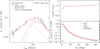 |
Fig. 1. Left: 3 GHz light curve of afterglow from structured jet at distance D = 42 Mpc, with sharp power-law structure (a = 4.5, b = 2.5; see Eqs. (1)–(2)), viewing angle θv = 22°, external density n = 3 × 10⁻³ cm−3, core jet with θj = 4°, Γc = 100, Eiso, c = 2 × 1052 erg, and with microphysics parameters p = 2.2, ϵe = 0.1 and ϵB = 10−4. The radio observations of GW170817 are also plotted and are compiled from Hallinan et al. (2017), Alexander et al. (2018), Margutti et al. (2018), Mooley et al. (2018a,b), Dobie et al. (2018). The respective contributions of the core jet (θ ≤ θj), the sheath and the total are plotted in dashed, dotted and solid red lines. The flux of the core jet computed with the simplified treatment described by Eq. (4) is also plotted in dashed blue line for comparison. Bottom right: peak flux of same structured jet as function of viewing angle θv (solid red line), peak flux of light curve from core jet only (dashed red line) or from sheath only (dotted red line), and peak flux of core jet as computed using scaling law in Eq. (6) (thin black line). Upper right: ratio of peak flux from whole outflow (core jet+sheath) to that of core jet only. |
As long as the kinetic energy and the Lorentz factor decay steeply with θ, the core jet is expected to dominate the flux at the peak whatever the viewing angle, even if the precise value of the total-to-core ratio at the peak may slightly vary depending on the details of the assumed lateral structure. Therefore, as our population model takes only the properties of the afterglow at the peak into account, that is, when it can be detected more easily, it is enough in the following to compute only the contribution from the core jet, while keeping in mind that it may slightly underestimate the total peak flux by a factor of1 ∼1.5.
The contribution from a top-hat core jet can efficiently be computed using the approximation suggested by Granot et al. (2002) to avoid the full integration over equal-arrival time surfaces. More precisely, we computed the flux  of a spherical ejecta with initial Lorentz factor Γc and kinetic energy Eiso, c as in Panaitescu & Kumar (2000), and we corrected it by defining the on-axis afterglow flux including the jet break:
 (3)
(3)
and by calculating the afterglow from any viewing angle as:
 (4)
(4)
with  and
and  where t is the source frame time. The latter correction, corresponding to the ratio of on-axis and off-axis arrival times is not included in Granot et al. (2002) and is found to improve the quality of the approximation. The corresponding light curve is plotted in Fig. 1 (left, blue dashed line) and corresponds well with the exact calculation.
2.2. An analytical model for afterglow peak properties
This afterglow calculation is standard for top-hat jets. Therefore analytical expressions for the afterglow properties at the peak are available. They depend slightly on the assumptions for a possible late jet lateral expansion. If lateral expansion is taken into account like in standard GRB afterglow theory, the peak flux of the radio light curve scales as (Nakar et al. 2002):
 (5)
(5)
as long as the spectral regime remains νm < ν < νc. This leads to the following expression2 of the peak flux at 3 GHz:
 (6)
(6)
where E52 = Eiso, c/1052 erg, θj, −1 = θj/0.1 rad, n−3 = n/(10−3 cm−3), ϵe, −1 = ϵe/10−1, ϵB, −3 = ϵB/10−3, θv, −1 = θv/0.1 rad and D100 = D/(100 Mpc), and where we assume p = 2.2. This scaling law is plotted in Fig. 1 (right, solid black line) and corresponds well with the detailed calculation. The expression of the corresponding peak time is also given by Nakar et al. (2002), assuming lateral expansion of the jet. However, even if late observations of GRB170817A may give some evidence for the lateral expansion of the core jet (for example the temporal decay index being ∼ − p, as found by Mooley et al. 2018a), it is not clear if this expansion should be as strong for a core jet embedded in a sheath as for a “naked” top-hat jet. Therefore, we also consider a limit case without lateral expansion. This only affects the peak flux slightly and Eq. (6) above remains a good approximation in both cases. On the other hand, it modifies the peak time, leading to:
 (7)
(7)
and
 (8)
(8)
where tb is the standard jet break time,
 (9)
(9)
The ratio of the peak times without and with lateral expansion is simply
 (10)
(10)
In the following, we use, unless otherwise noted, Eqs. (6)–(8) to estimate the peak flux and peak time of the radio afterglow from a binary neutron star merger.
2.3. Physical parameters of the jet and their intrinsic distribution
To generate a population of jet afterglows we had to fix the various parameters appearing in Eqs. (6)–(8). We first defined a set of “fiducial distributions” for these parameters. These are summarized in Table 1 and have been chosen as follows.
Fiducial population model parameter distributions.
Core jet isotropic equivalent kinetic energy Eiso, c: we adopted a broken power-law distribution, which we deduced directly from the gamma-ray luminosity function of cosmological short GRBs, assuming a standard rest frame duration ⟨τ⟩ = 0.2 s and a standard efficiency fγ = 0.2 (Beniamini et al. 2016) so that Eiso, c ∼ Lγ ⟨τ⟩/fγ, leading to a density of probability
 (11)
(11)
where ϕ is normalized to unity. We fixed Emin = 1050 erg and Emax = 1053 erg. Luminosity functions for short GRBs were deduced based on observations from several teams (e.g., D’Avanzo et al. 2014; Wanderman & Piran 2015; Ghirlanda et al. 2016). For our fiducial model, we adopted that of Ghirlanda et al. (2016) with α1 = 0.53, α2 = 3.4 and a break luminosity of Lb = 2 × 1052 erg s−1 leading to Eb = 2 × 1052 erg.
Jet opening angle θj: for simplicity we assumed a single value θj = 0.1 rad, which appears to be representative of the typical value found by fitting the afterglow light curve of GW170817 (e.g., Gill & Granot 2018; van Eerten et al. 2019), by the VLBI observations of the remnant (Mooley et al. 2018c) and also consistent with the results of prior short GRB afterglow fitting (Fong et al. 2015) and short GRB-BNS merger rate comparisons (Beniamini et al. 2019).
External density n: most BNS mergers are expected to occur in low density environments due to a long merger time, as assessed by the significant offsets of short GRB sources from their host galaxies (e.g., Nakar 2007; Troja et al. 2008; Fong et al. 2010; Church et al. 2011; Berger 2014). In the case of GW170817, afterglow fitting typically leads to n ∼ 10−3 cm−3, which is in agreement with the estimation of the HI content of the host galaxy NGC 4996 (Hallinan et al. 2017). The external densities observed in short GRBs cover the interval 10−3 − 1 cm−3 (Berger 2014), but this is probably biased towards high densities, which favor afterglow detection. In this paper we consider n ∼ 10−3 cm−3 as typical and set, therefore, a log-normal of mean 10−3 cm−3 with a standard deviation of 0.75 as the fiducial density distribution.
Microphysics parameters: we set the value of ϵe at 0.1. This is generally done in GRB afterglow modeling (Wijers & Galama 1999; Panaitescu & Kumar 2001; Santana et al. 2014; Beniamini & van der Horst 2017; D’Avanzo et al. 2018). Also, this value has been adopted or found in the fitting of the afterglow of GW170817 (e.g., van Eerten et al. 2019; Margutti et al. 2018; Nakar et al. 2018; Xie et al. 2018), and it is consistent with particle shock-acceleration simulations (Sironi & Spitkovsky 2011). Similarly, we set p at 2.2, which is also a common value used in GRB afterglow models and which is in agreement with shock-acceleration theory in the relativistic regime (e.g., Sironi et al. 2015). In the case of GW170817 this value can be directly measured from multi-wavelength observations (Mooley et al. 2018a,b; van Eerten et al. 2019). Finally, more diversity is generally expected for ϵB. We assumed a log-normal distribution similar to the one adopted for n with the additional constraint that ϵB is restricted to the interval [10−4, 10−2].
In Sect. 4.2 we consider possible alternatives to these fiducial distributions. In particular, we discuss the impact of substantial uncertainties in the distribution of kinetic energy, ϕ(Eiso, c), either due to the difficulty in measuring the luminosity function of short GRBs, or in simplifying assumptions regarding the duration and the efficiency of the prompt GRB emission. We also explore different values of the jet opening angle θj. As for the external density, we examine the effect of a change in the mean circum-merger density of the population of mergers.
3. From the intrinsic to the observed population: GW and radio joint detection
3.1. GW detection criterion
The signal-to-noise ratio (S/N, denoted by ρ) of a GW inspiral signal in a single LIGO-Virgo-type interferometer can be written as  (Finn & Chernoff 1993), where D is the luminosity distance to the binary, ℳ is the chirp mass of the binary, SI is a quantity depending only on the sensitivity profile of the interferometer, and Θ2 represents the dependence of the signal to the binary sky position (θ, ϕ) and orientation (θv, ξ) with respect to the plane of the interferometer. Again, θv is the angle of the line of sight to the binary polar direction, which we also assumed is the jet-axis direction. The function Θ2 admits a global maximum of
  corresponding to an optimally positioned and oriented source (binary at the zenith and polar axis orthogonal to the instrument’s arms). This optimal binary can be detected out to a distance known as the horizon H of the instrument, which depends on the S/N threshold for detection, taken to be ρ0 = 8 for the LVC network. We may thus rewrite the S/N in the following manner:
 (12)
(12)
In a full population study, one would have to draw all four angles and evaluate this criterion in every case. We chose to reduce the number of parameters to two: D and θv, as these are the ones relevant to the afterglow. Thus, we were compelled to review this criterion by averaging Θ2 on the sky-position (θ, ϕ) and polarization angle ξ. This is done readily from the expression given in Finn & Chernoff (1993; Eq. (3.31)) and it is found analytically that:
 (13)
(13)
Hence, we chose to use the following criterion to determine those binaries of inclination θv and distance D which are detectable in GW on average in the sky:
 (14)
(14)
which is:
 (15)
(15)
where we have denoted  for the sky-position-averaged horizon.
Averaging Θ2 on inclination angle θv and imposing an S/N threshold as in Eq. (14) would lead to the simple detection criterion of D < R, where R is the range of the instrument, that is, the maximum distance at which a binary can be detected on average in sky-position and in orientation. The range is linked to the horizon by H = 2.26R.
The criterion of Eq. (15) is valid for a detection using a single instrument. Instead, GW detection by the interferometer network is based on multi-instrument analysis, and is, thus, more complicated than the one described by our criterion. Furthermore, as was illustrated in the case of GW170817, true joint GW-AG detection requires pinpointing the source through the detection of the kilonova counterpart3, which in turn involves a small enough localization map from the GW data, and our criterion should incorporate this. We chose a simple localization criterion by supposing that a source is localized if it is detectable (once again on average) by the two most sensitive interferometers of the network. Thus our detection-localization criterion is that of Eq. (15), with the horizon of the second most sensitive instrument of the network, that is, the LIGO-Hanford instrument. Table 2 reports the corresponding values taken for our study for the LVC O2, O3 runs, and for the design interferometers.
Horizons used for GW detection-localization criterion in our study.
In this framework, it can be shown that assuming homogeneity of the sources within the horizon and isotropy of the binary polar direction, the mean viewing angle of GW-detected events is ∼38° and the fraction of GW-detected events among all mergers is ∼29%, both regardless of the horizon value. This latter fraction is, thus, an absolute maximum for the fraction of mergers to be jointly detected in both radio and GW channels.
3.2. Radio detection criterion
The detection criterion in the radio band is simply for the 3 GHz peak flux, as determined by our models, to be larger than the sensitivity of the radio array available for follow-up at the time of consideration, which we denote by s. We note that this is a criterion aimed rather at detectability than detection. True detection only occurs if observations are pursued for long enough after the GW merger signal, as the flux rises to its maximum. We also note that events which are marginally detectable would only provide poor astrophysical output because the inference of jet parameters requires the fitting of an extended portion of the radio afterglow light curve.
We took three typical radio sensitivities reflecting the present and future capabilities of radio arrays: (i) the Karl Jansky Very Large Array (VLA) at s = 15 μJy, (ii) the phase I of the Square Kilometer Array (SKA1, Braun 2014), at s = 3 μJy, and (iii) phase II of the SKA (SKA2) and the Next Generation VLA (ngVLA, Selina et al. 2018), both at s = 0.3 μJy. The combination of this radio detection criterion with that of the GW domain (Eq. (15)) constituted our criterion for the joint detection of mergers.
In the sequel, we referred to a jointly GW and radio detectable population by using the names of the corresponding LVC run and limiting radio facility, as in “the joint population of the O3 and VLA configuration”. The corresponding GW interferometer horizons and radio sensitivities can be found respectively in Table 2 and in the paragraph above.
4. Results: detection rates and properties of the detected population
4.1. Fiducial model
In this section, we describe the population of events detected jointly in the GW and radio domains. For this purpose, we used a Monte Carlo approach in which we simulated N > 106 binary systems within the sky-averaged horizon  using the parameter distributions of the fiducial model given in Sect. 2.3. By applying the detection criteria described in Sect. 3, we obtained NGW systems detected by the GW interferometer network and Njoint systems which are also detectable by radio telescopes by their afterglows. Then we studied the properties of the sample of joint GW and radio detectable events.
4.1.1. Rate of joint GW and radio detectable events
Starting from the fraction fGW = NGW/N ∼ 29% of binary systems detected by the LVC (Sect. 3.1), we then estimated which fraction Njoint/NGW of those events would also produce a detectable radio afterglow.
This fraction is shown in Fig. 2 (left) as a function of the GW horizon and for the VLA, SKA1 and SKA2/ngVLA limiting sensitivities. In the design configuration of the LVC network, 75% (resp. 2 times) more events are detectable by SKA1 (resp. SKA2/ngVLA) than by the VLA.
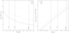 |
Fig. 2. Left: detectable fraction of radio afterglows among gravitational wave events as function of the horizon distance |

The number of joint event detections normalized to the O3-VLA configuration is represented in Fig. 2 (right). The number of joint detections behaves approximately as Hα, with α < 3 because of the reduction in radio detection efficiency when the distance is increased (Fig. 2, left). We find α ≃ 2.4 (resp. 2.6, resp. 2.8) for the VLA (resp. SKA1, resp. SKA2/ngVLA).
As illustrated in Fig. 2 (left), we find that the fraction of detected events decreases from 43% (O2) to 31% (O3) with the VLA limiting sensitivity. However the absolute number of detections increases (Fig. 2, right). With the design-SKA1 configuration, a fraction of 35% of GW events can lead to a radio detection. With regard to the much higher sensitivities that may be reached after 2030, more than a half of GW events may become detectable in the radio band. Indeed we found a percentage of 63% of detectable joint events in the design-SKA2/ngVLA configuration.
For the purposes of a comprehensive survey, the number of GW and jointly detected events per continuous year of GW network operation for future detector configurations can be found in Table 3, where we have used the horizons of Table 2 and our fiducial model.
Number of detectable events per continuous year of GW network operation.
4.1.2. Distance and viewing angle
The distributions of distances are shown in Fig. 3 for the O2-VLA and O3-VLA configurations, as well as for the entire GW population. In this figure, the distributions are not normalized to unity so as to show the decrease in the fraction of joint event as the horizon increases. It can be observed that as a result of the GW and radio detection thresholds, sources are progressively lost when the distance increases so that this distribution exhibits a near linear increase (as opposed to the dN/dD ∝ D2 of the intrinsic homogeneous population). Up to  , all events are detected in GW, regardless of their orientation4 and the only selection is due to the radio sensitivity. Near the horizon, the maximum viewing angle allowing GW-detection is
  , which produces a strict decrease of event density.
Figure 4 shows the distribution of the viewing angles. For the joint events, the peak of the distribution takes place at small viewing angles θv ∼ 15−20° as a result of the rapid decline of the peak flux with angle ( ), and about 39% (resp. 47%) of the events would be seen with a viewing angle θv < 20° for O2-VLA (resp. O3-VLA), the angle at which the GW170817 event was likely to have been seen. As shown in Fig. 5 (left), the mean viewing angle of the jointly observed events strongly depends on the GW horizon and the radio sensitivity. It appears that even if the radio sensitivity is not substantially improved while the GW interferometers reach their design horizons, a significant number of events would still be observable off-axis. The increasing and decreasing phases of the afterglows of these events would allow for an improved study of the jet structure, which is better revealed by off-axis events. Figure 5 (right) shows the fraction of on-axis events (θv ≤ θj) within the joint detections. It increases from 4.0% (O2-VLA) to 5.3% (O3-VLA).
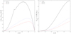 |
Fig. 3. Left: differential distribution of distances (normalized to the sky-position-averaged horizon) of events in total GW population (full line), and detectable jointly in O2-VLA (dotted line) and O3-VLA (dashed line) configurations. Right: cumulative distribution of same events. Distributions have been normalized to the fraction of jointly detected events among all GW-detected events, see text for details. |
4.1.3. Peak times, peak fluxes and synchrotron spectral regime
The distributions of peak times and peak fluxes in the O3-VLA configuration are represented in Fig. 6. The fraction of events with a peak time of fewer than 150 days (as observed in GRB 170817A) is 55% without jet expansion and 81% with lateral expansion. The distribution in peak flux is shown for all sources which are detected in gravitational waves within the sky-position-averaged horizon of O2, O3 and design instruments. It appears clear that for the present VLA sensitivity, most radio afterglows cannot be detected. This explains why improving the sensitivity of the future ngVLA would have such an impact on the joint detection rates, as shown in Fig. 2.
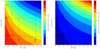 |
Fig. 5. Left: mean viewing angle of jointly detected events, as function of horizon and radio sensitivity s. Values of H for O2, O3 and design instruments, as well as s for VLA, SKA1 and SKA2/ngVLA, are indicated as dashed lines. Right: fraction of on-axis events (defined by θv ≤ θj) among jointly detected events in same H–s diagram. |
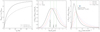 |
Fig. 6. Left: cumulative distributions of peak times of radio afterglows for jointly detected events in O3-VLA configuration, assuming jet with (solid line) or without (dashed line) lateral expansion. Middle: differential distribution of peak fluxes of GW-detected events assuming horizon for O2 (dotted line), O3 (dashed line) and design (full line) configurations of GW interferometers. The radio sensitivities for VLA, SKA1 and SKA2/ngVLA are indicated for comparison. Right: differential distribution of maximum proper motion for jointly detected events assuming O2-VLA (dotted line), O3-VLA (dashed line), design-SKA1 (full line) configurations. The dotted vertical line shows the lower limit for detection of the proper motion. |
The scaling law used to compute the radio emission at the peak assumes that the observing frequency remains in the same spectral regime of the slow-cooling synchrotron spectrum, that is, νm < ν < νc, and above the absorption frequency. Using our more detailed calculation of the radio afterglow from the core jet (Eq. (4) and accompanying text), we can ascertain if this condition is fulfilled for the bulk of the population. However, for mergers in high density environments (larger than 10 cm−3), this condition is no longer met as the absorption frequency νa and the injection frequency νi may be larger than the radio frequency at early times. For an event with n = 10 cm−3 and θv ∼ 40° (the mean viewing angle of the GW-detected population), the radio frequency typically meets the injection break at around 30 days (resp. before 10 days). In this case, chromatic light curves are expected.
4.1.4. Proper motion
Another independent observable is the proper motion of the remnant, which can be readily accessible to VLBI measurements as illustrated in the case of GRB170817A (Mooley et al. 2018c; Ghirlanda et al. 2019). However, a VLBI network can only measure the proper motion of a source if the total displacement of the source over the time it is detectable by the array is larger than the angular resolution of the network. For our purposes, we chose to simplify this criterion and adopt a dual condition on the flux (Fp > sVLBI), as well as on the instantaneous proper motion μmax (requiring that μmax > μlim) of the remnant at the peak of the afterglow. Here, we adopted a limiting proper motion of μlim = 3 μas/day, in coherence with the uncertainties quoted in Mooley et al. (2018c), Ghirlanda et al. (2019).
An upper limit of the proper motion was obtained based on the assumption that the core jet contribution dominates at the peak of the radio light curve, and that the shocked region at the front of this core jet constitutes the visible remnant of the merger. In first approximation, afterglows from jets peak when the observer enters the focalization cone of the radiation, that is, Γ ∼ 1/θv. For an off-axis observer, we estimated, therefore, the maximum proper motion to be:
 (16)
(16)
with
 (17)
(17)
Thus, for a given value of the viewing angle, there is a maximum distance beyond which the measurement of the proper motion is not possible. It is given by
 (18)
(18)
The distribution of μmax is shown in Fig. 6 (right) for O2, O3 and design-level detectable GW events respecting the VLBI flux criterion. Here, we have take sVLBI = 15 μJy, which represents a limiting S/N of ∼3 with the level of noise reported in Mooley et al. (2018c), Ghirlanda et al. (2019) for the e-MERLIN and High Sensitivity Array networks. Within the O2-VLA (resp. O3-VLA, resp. design-VLA) populations, the measurement of the proper motion is possible in only 79% (resp. 64%, resp. 42%) of the jointly-detectable events.
Finally, we represent in Fig. 7 various plots connecting two observable quantities: (θv, D), (θv, Fp, 3 GHz), (θv, tp) and (D, μmax). The grey dots correspond to events detectable in GW and the red crosses correspond to those detectable in both GW and radio. In the (θv, D) diagram, the limiting distance for the measurement of the proper motion (Eq. (18)) is shown. This figure illustrates the various observational biases discussed in this section, and especially the bias towards small viewing angles, mainly due to the limiting sensitivity of radio telescopes.
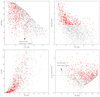 |
Fig. 7. Predicted samples of GW-detected (dots) and jointly detected (crosses) mergers in planes of various pairs of observables, for O3-VLA configuration. Upper left: distance and viewing angle, and maximum distance at which the proper motion can be measured (Dmax(θv), see Eq. (18), green dotted line). Upper right: peak flux and viewing angle. Lower left: time of radio afterglow peak (assuming lateral expansion of jet) and viewing angle. Lower right: maximum remnant proper motion and distance, and limiting proper motion μlim (green dotted line). |
4.1.5. Kinetic energy, external density and microphysics parameters
The distributions of kinetic energy Eiso, c and external density n, which are not directly observable but may result from fits of the afterglow, are shown in Fig. 8. In each case, the distributions of jointly detected events have been compared to total GW detections. As the GW selection is independent of the kinetic energy and density, these distributions are the intrinsic distributions of our population model (Table 1). As could be expected, the detection of mergers leading to a relativistic core jet with a large Eiso, c is favored. In jointly detectable mergers, the energy distribution approximately remains a broken power-law, but the respective indices below and above the break decrease from 0.53 to 0.2 and 3.4 to 3.2, respectively. After applying the joint detectability criterion, the external density distribution is simply shifted to higher densities, as the mean value is increased by a factor of ∼2.2. The distribution of the microphysics parameter ϵB is very similar to that of the density, because both parameters appear with the same power in the peak flux (Eq. (6)).
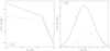 |
Fig. 8. Differential distribution of core jet kinetic energy (left) and external medium density (right) of entire GW population (full) and jointly detected events (dashed), in O3-VLA configuration. Distributions are normalized to fraction of jointly detected events among all GW-detected events, see text for details. |
We find that the Lorentz factor of the jet at the time of peak flux has a median value of ∼4. This is consistent with the approximate jet core de-beaming relation Γ ∼ (θv−θj)−1 for a jet with θj = 0.1 rad seen with the mean viewing angle θv ∼ 24° for the O3-VLA configuration. This justifies keeping microphysics parameters representative of shock-acceleration in the ultra-relativistic regime for the whole population.
4.2. Impact of the population model uncertainties on the predicted population
4.2.1. Jet energy distribution and opening angle
Here we consider alternatives to our fiducial population model. With a distribution of jet energy that increases below the break (i.e., taking α1 < 0 in Eq. (11)) as would be obtained from the short GRB luminosity function of Wanderman & Piran (2015) (α1 = −0.9) and still assuming the same standard values for the duration and efficiency, the fraction of events detectable with the VLA would typically be three times smaller: 15% for O2 and 10% for O3 compared to 43% and 31% with α1 = 0.5. The viewing angle and peak times would also be strongly affected, showing mean θv’s for O2 (resp. O3) at only 17° (resp. 14°), 98% (resp. 99%) of afterglows peaking before 150 days in the jet expansion hypothesis, and 90% (resp. 93%) without lateral expansion.
These results were obtained assuming a typical value fγ = 20% for gamma-ray efficiency but one cannot exclude that fγ may vary from from less than 1% to more than 20%. Estimates of fγ from afterglow fitting have indeed been found to cover a large interval (e.g., Lloyd-Ronning & Zhang 2004; Zhang et al. 2007). Thus, the three orders of magnitude in isotropic gamma-ray luminosity could partially result from differences in efficiency, the jet isotropic kinetic energy being restricted to a smaller interval. Figure 9 shows the effect of increasing the minimum kinetic energy Emin from 1050 to 1052 erg in the energy function deduced from the short GRB luminosity function of Wanderman & Piran (2015) on the detected fraction, the mean viewing angle and the fraction of afterglows to peak before 150 days. As could be expected, when the minimum kinetic energy was increased, the results came closer to those of the fiducial model in which the energy distribution function decreases below the peak.
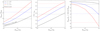 |
Fig. 9. Left: fraction of joint events among GW events assuming short GRB luminosity function from Wanderman & Piran (2015) for different values of minimum kinetic energy Em (full lines), and for our fiducial model (dashed lines), in O3-VLA configuration. Results have been plotted for different values of the jet opening angle θj = 0.05, 0.1 and 0.15 rad (red, black and blue lines respectively). Middle: mean viewing angle (same color coding). Right: fraction of joint events with peaks earlier than 150 days post-merger, with hypothesis of jet lateral expansion, same color coding. |
We also show in Fig. 9 the effect of changing the typical value of the jet opening angle from 0.1 to 0.05 or 0.15 rad. When θj = 0.05 (resp. 0.15), the detected fraction decreases (resp. increases) to 19% (resp. 40%), the mean viewing angle decreases (resp. increases) by 4°, and the peak of the light curve generally occurs later (resp. earlier).
4.2.2. External density distribution and microphysics
The afterglow peak flux depends greatly on the density of the circum-merger medium, as can be seen from Eq. (6). Therefore, the ability to detect the afterglows of a population of mergers depends strongly on the density of the media hosting the binaries upon merger. This is illustrated in Table 4, where we give this fraction for different external density distribution central values. These figures were calculated using the semi-analytical model (Eq. (4)), taking into account the full synchrotron spectrum including self-absorption.
If there is a significant population of fast-merging neutron star binaries, as proposed by Matteucci et al. (2014), Hotokezaka et al. (2015), Vangioni et al. (2016), Beniamini & Piran (2016), for example, these should merge in higher density environments, producing brighter afterglows and offering the possibility to notably contribute to the observed population even if they are intrinsically fewer in number. With a density distribution centered at n = 10 cm−3, and the other parameters taking their fiducial values, 99% of GW events produce detectable radio afterglows in the O3-VLA configuration.
The microphysics parameter ϵB enters in Eq. (6) with the same power as the external density. Moreover, our fiducial choices for the distribution of these two quantities are nearly the same (with simply a limit in range for ϵB) so that changing its central value affects the detected fraction in the same way.
5. Discussion and conclusion
We studied the population of binary neutron star mergers to be observed jointly through GW and their radio afterglows in future multi-messenger observing campaigns. To do so, we have assumed a likely population of mergers inspired by prior short GRB science, and simulated the GW and jet-dominated radio afterglow emissions from these. We have made predictions on the rates of such future events, and on how the observables from these events are expected to be distributed among themselves.
In the case of the ongoing O3 run of the LVC, and assuming our fiducial set of parameters (see Table 1), we predict that ∼30% of GW events should have a radio afterglow detectable by the VLA. These joint events should have mean viewing angles of ∼24°, and should peak earlier than 150 days post-merger in ∼80% of cases, assuming lateral expansion of the jet.
As illustrated in the 170817 event, the lateral material may also contribute to the peak flux of the radio afterglow. Figure 1 (right) shows that this may increase the peak flux by a factor of up to 1.5. In this case, our O3 predictions are revised to a fraction of 36% of events with detectable afterglow and a similar mean viewing angle of 25°.
5.1. Detecting the detectable events
Throughout this work, we have applied a threshold on the GW S/N and radio afterglow peak flux to label an event as jointly detected. Thus our study concerns the class of detectable events. The fraction of these detectable events that can actually be detected heavily depends on the accuracy of the localization, which is related to the size of the localization skymap provided by the GW network, the possible detection of an associated GRB, and the efficiency of the search for a kilonova in terms of covered sky area and limiting magnitude.
Assuming that all neutron star mergers produce a kilonova, and even taking into account a probable anisotropy of the emission, it is expected that 100% of kilonovae are detectable during O3 for a limiting magnitude of 21 (Duque et al. 2019; Mochkovitch et al. in prep.). However, the search for the kilonova becomes complicated due to the large localization skymaps of GW events. These error boxes can be improved in the case when an associated GRB is being detected, which should, however, tend to remain rare (see Sect. 4.1.2 and Beniamini et al. 2019). During O3, existing facilities with large fields of view in the optical band are experiencing difficulty in covering 100% of ≳1000 deg2 skymaps with a deep limiting magnitude, especially in the southern sky. Instruments such as the Zwicky Transient Facility (Bellm et al. 2019) cover the northern sky down to magnitude r ∼ 20.5.
On the other hand, when the LIGO/Virgo instruments will have achieved their design sensitivities, it is expected that one or two new interferometers will join the GW network: KAGRA (Kagra Collaboration 2019) and Ligo-India (Iyer 2015). This should lead to a significant improvement in localization. In addition, the deep coverage of even large error boxes will be made possible by new facilities such as the Large Synoptic Survey Telescope (Ivezic et al. 2008). Nevertheless, there are other difficulties related to the search for the kilonova: kilonova/host galaxy contrast at large distances, possible large offsets, availability of a photometric and spectroscopic follow-up of the candidates, etc. In this context, it is clear that the efficiency of the search for kilonovae will always remain below 100%, but should increase with time and may potentially be high in the design configuration of the GW network.
Even assuming the localization has been acquired thanks to the detection of a kilonova, a continuous monitoring of the remnant up to ∼150 days may be necessary to detect the peak of the radio afterglow, in the case of marginally detectable events. Even then, only events with peaks somewhat larger than the radio threshold should yield observations of astrophysical interest because extended observations of the rise, peak and decay of the afterglow are necessary to resolve the structure and dynamics (e.g., expansion) of the ultra-relativistic jet, as illustrated by the case of GRB170817A.
As also illustrated in the case of GRB170817A, VLBI measurements are instrumental in assessing the presence and resolution of the jet structure. Therefore, an even more restrictive criterion for full event characterization might be the detectability of the remnant proper motion. As we demonstrated in Sect. 4.1.4, this would primarily decrease the fraction of events, especially in the context of design GW detectors.
5.2. Constraining the BNS population and short GRBs with radio afterglows
We have studied the sensitivity of the expected distributions of afterglow observables to the population parameters, as well as the radio and GW detector configurations. In particular, we have shown the uncertainties on the rates and typical viewing angles of these events which have been inherited from the uncertainties on the luminosity function of short GRBs and of the density of the media hosting the mergers.
In Sects. 4.1.1 and 4.1.2 we discussed the combined influence of increasing the radio and GW detector sensitivity on the rate and viewing angle of the events. At this stage, both improvements would be beneficial as the predicted rate in the current O3-VLA configuration is well below 50% of joint events among GW events.
As the GW horizon increases, more events will be seen on-axis. In the case of an opening angle of 0.1 rad and in the likely short-term evolution of the detector configuration from O3-VLA (current) to design-VLA (early 2020s), we predict that 5% to 10% of events should be seen on-axis, increasing the probability of a GRB counterpart in addition to the GW and afterglow. This figure is fully consistent with that announced in Beniamini et al. (2019) for events with a GW+GRB association. In fact, as a GW+classical GRB association is equivalent to an on-axis event, one may measure the opening angle of typical GRB jets by considering the ratio of GW events with afterglow counterpart only to events with both afterglow and GRB, thus exploiting the new possibility of observing afterglows without detecting the GRB.
More generally, a population of observed events corresponds to an intrinsic population of mergers. Thus, a comparison of a statistical number of joint event observations to our predicted distributions is a means of measuring fundamental parameters of the population of mergers, and of constraining GRB quantities, such as their energy function.
Finally, future facilities such as the SKA may bring detections of orphan radio afterglows through deep radio surveys. These would not be subject to the GW criterion and may probe another sub-population of mergers, bringing yet another class of constraints upon these phenomena.
In conclusion, regardless of the evolution of GW and radio detectors, multi-wavelength afterglows will remain instrumental in the study of binary neutron star mergers as windows on both their environment and their role as progenitors of short GRBs. They will bring invaluable insight at the level of the population of mergers and on an event-to-event basis, provided the sources may be accurately localized in the sky.
See Sect. 5 for a short discussion of the effect of this on the fraction of detectable events.
We don’t take into account the effect of redshift, as the events at play here are within the GW horizon distance of first generation interferometers, i.e., with z ≤ 0.1.
This was not achieved in the recent merger candidates S190425z and S190426c (Ligo Scientific Collaboration & VIRGO Collaboration 2019a,b), see Sect. 5 for more discussion on this.
Beyond this distance, events are detected in GW only if θv ≤ θmax with  . The differential distribution of distances for the GW events thus transitions from ∝D2 before
  to a non-quadratic form afterwards, producing the small peak seen in Fig. 3. This, of course, is only a consequence of our simplified GW sky-averaged detection criterion (Eq. (15)).
Acknowledgments
The authors acknowledge financial support from the Centre National d’Études Spatiales (CNES), and thank Paz Beniamini for useful discussions.
References
- Abbott, B. P., Abbott, R., Abbott, T. D., et al. 2017, Phys. Rev. Lett., 119, 161101 [NASA ADS] [CrossRef] [PubMed] [Google Scholar]
- Abbott, B. P., Abbott, R., Abbott, T. D., et al. 2018, Liv. Rev. Rel., 21, 3 [NASA ADS] [CrossRef] [Google Scholar]
- Abbott, B. P., Abbott, R., Abbott, T. D., et al. 2019, Phys. Rev. X, 9, 011001 [Google Scholar]
- Alexander, K. D., Margutti, R., Blanchard, P. K., et al. 2018, ApJ, 863, L18 [NASA ADS] [CrossRef] [Google Scholar]
- Bellm, E. C., Kulkarni, S. R., Graham, M. J., et al. 2019, PASP, 131, 018002 [NASA ADS] [CrossRef] [Google Scholar]
- Beniamini, P., & Piran, T. 2016, MNRAS, 456, 4089 [NASA ADS] [CrossRef] [Google Scholar]
- Beniamini, P., & van der Horst, A. J. 2017, MNRAS, 472, 3161 [NASA ADS] [CrossRef] [Google Scholar]
- Beniamini, P., Nava, L., & Piran, T. 2016, MNRAS, 461, 51 [NASA ADS] [CrossRef] [Google Scholar]
- Beniamini, P., Petropoulou, M., Barniol Duran, R., & Giannios, D. 2019, MNRAS, 483, 840 [NASA ADS] [CrossRef] [Google Scholar]
- Berger, E. 2014, Annu. Rev. Astron. Astrophys., 52, 43 [Google Scholar]
- Braun, R. 2014, SKA Technical Document, SKA-TEL.SCI-SKO-SRQ-001 [Google Scholar]
- Cantiello, M., Jensen, J. B., Blakeslee, J. P., et al. 2018, ApJ, 854, L31 [NASA ADS] [CrossRef] [Google Scholar]
- Church, R. P., Levan, A. J., Davies, M. B., & Tanvir, N. 2011, MNRAS, 413, 2004 [NASA ADS] [CrossRef] [Google Scholar]
- Coulter, D., Foley, R., Kilpatrick, C., et al. 2018, APS April Meeting Abstracts, 2018, D16.002 [Google Scholar]
- Cowperthwaite, P. S., Berger, E., Villar, V. A., et al. 2017, ApJ, 848, L17 [NASA ADS] [CrossRef] [Google Scholar]
- D’Avanzo, P., Salvaterra, R., Bernardini, M. G., et al. 2014, MNRAS, 442, 2342 [NASA ADS] [CrossRef] [Google Scholar]
- D’Avanzo, P., Campana, S., Salafia, O. S., et al. 2018, A&A, 613, L1 [NASA ADS] [CrossRef] [EDP Sciences] [Google Scholar]
- Dobie, D., Kaplan, D. L., Murphy, T., et al. 2018, ApJ, 858, L15 [NASA ADS] [CrossRef] [Google Scholar]
- Duffell, P. C., Quataert, E., Kasen, D., & Klion, H. 2018, ApJ, 866, 3 [NASA ADS] [CrossRef] [Google Scholar]
- Duque, R., Mochkovitch, R., & Daigne, F. 2019, Proceedings of Science [Google Scholar]
- Evans, P. A., Cenko, S. B., Kennea, J. A., et al. 2017, Science, 358, 1565 [NASA ADS] [CrossRef] [Google Scholar]
- Finn, L. S., & Chernoff, D. F. 1993, Phys. Rev. D, 47, 2198 [NASA ADS] [CrossRef] [Google Scholar]
- Fong, W., Berger, E., & Fox, D. B. 2010, ApJ, 708, 9 [NASA ADS] [CrossRef] [Google Scholar]
- Fong, W., Berger, E., Margutti, R., & Zauderer, B. A. 2015, ApJ, 815, 102 [NASA ADS] [CrossRef] [Google Scholar]
- Ghirlanda, G., Salafia, O. S., Pescalli, A., et al. 2016, A&A, 594, A84 [NASA ADS] [CrossRef] [EDP Sciences] [Google Scholar]
- Ghirlanda, G., Salafia, O. S., Paragi, Z., et al. 2019, Science, 363, 968 [NASA ADS] [CrossRef] [Google Scholar]
- Gill, R., & Granot, J. 2018, MNRAS, 478, 4128 [NASA ADS] [CrossRef] [Google Scholar]
- Goldstein, A., Veres, P., Burns, E., et al. 2017, ApJ, 848, L14 [NASA ADS] [CrossRef] [Google Scholar]
- Gottlieb, O., Nakar, E., & Piran, T. 2018, MNRAS, 473, 576 [NASA ADS] [CrossRef] [Google Scholar]
- Gottlieb, O., Nakar, E., & Piran, T. 2019, MNRAS, 488, 2405 [NASA ADS] [CrossRef] [Google Scholar]
- Granot, J., Panaitescu, A., Kumar, P., & Woosley, S. E. 2002, ApJ, 570, L61 [NASA ADS] [CrossRef] [Google Scholar]
- Haggard, D., Nynka, M., Ruan, J. J., et al. 2017, ApJ, 848, L25 [NASA ADS] [CrossRef] [Google Scholar]
- Hallinan, G., Corsi, A., Mooley, K. P., et al. 2017, Science, 358, 1579 [NASA ADS] [CrossRef] [Google Scholar]
- Hotokezaka, K., Piran, T., & Paul, M. 2015, Nat. Phys., 11, 1042 [CrossRef] [Google Scholar]
- Hotokezaka, K., Kiuchi, K., Shibata, M., Nakar, E., & Piran, T. 2018, ApJ, 867, 95 [NASA ADS] [CrossRef] [Google Scholar]
- Ivezic, Z., Axelrod, T., Brandt, W. N., et al. 2008, Serb. Astron. J., 176, 1 [NASA ADS] [CrossRef] [Google Scholar]
- Iyer, B. 2015, APS April Meeting Abstracts, 2015, J13.001 [Google Scholar]
- Kagra Collaboration (Akutsu, T., et al.) 2019, Nat. Astron., 3, 35 [NASA ADS] [CrossRef] [Google Scholar]
- Kasliwal, M. M., Nakar, E., Singer, L. P., et al. 2017, Science, 358, 1559 [NASA ADS] [CrossRef] [Google Scholar]
- Lamb, G. P., & Kobayashi, S. 2017, MNRAS, 472, 4953 [NASA ADS] [CrossRef] [Google Scholar]
- Lazzati, D., Deich, A., Morsony, B. J., & Workman, J. C. 2017, MNRAS, 471, 1652 [NASA ADS] [CrossRef] [Google Scholar]
- Ligo Scientific Collaboration & VIRGO Collaboration 2019a, GRB Coordinates Network, 24168, 1 [Google Scholar]
- Ligo Scientific Collaboration & VIRGO Collaboration 2019b, GRB Coordinates Network, 24237, 1 [Google Scholar]
- Lloyd-Ronning, N. M., & Zhang, B. 2004, ApJ, 613, 477 [NASA ADS] [CrossRef] [Google Scholar]
- Lyman, J. D., Lamb, G. P., Levan, A. J., et al. 2018, Nat. Astron., 2, 751 [NASA ADS] [CrossRef] [Google Scholar]
- Margutti, R., Berger, E., Fong, W., et al. 2017, ApJ, 848, L20 [NASA ADS] [CrossRef] [Google Scholar]
- Margutti, R., Alexander, K. D., Xie, X., et al. 2018, ApJ, 856, L18 [NASA ADS] [CrossRef] [Google Scholar]
- Matteucci, F., Romano, D., Arcones, A., Korobkin, O., & Rosswog, S. 2014, MNRAS, 438, 2177 [NASA ADS] [CrossRef] [Google Scholar]
- Mooley, K. P., Frail, D. A., Dobie, D., et al. 2018a, ApJ, 868, L11 [NASA ADS] [CrossRef] [Google Scholar]
- Mooley, K. P., Nakar, E., Hotokezaka, K., et al. 2018b, Nature, 554, 207 [NASA ADS] [CrossRef] [PubMed] [Google Scholar]
- Mooley, K. P., Deller, A. T., Gottlieb, O., et al. 2018c, Nature, 561, 355 [NASA ADS] [CrossRef] [PubMed] [Google Scholar]
- Nakar, E. 2007, Phys. Rep., 442, 166 [NASA ADS] [CrossRef] [Google Scholar]
- Nakar, E., Piran, T., & Granot, J. 2002, ApJ, 579, 699 [NASA ADS] [CrossRef] [Google Scholar]
- Nakar, E., Gottlieb, O., Piran, T., Kasliwal, M. M., & Hallinan, G. 2018, ApJ, 867, 18 [NASA ADS] [CrossRef] [Google Scholar]
- Palmese, A., Hartley, W., Tarsitano, F., et al. 2017, ApJ, 849, L34 [NASA ADS] [CrossRef] [Google Scholar]
- Panaitescu, A., & Kumar, P. 2000, ApJ, 543, 66 [NASA ADS] [CrossRef] [Google Scholar]
- Panaitescu, A., & Kumar, P. 2001, ApJ, 560, L49 [NASA ADS] [CrossRef] [Google Scholar]
- Pian, E., D’Avanzo, P., Benetti, S., et al. 2017, Nature, 551, 67 [NASA ADS] [CrossRef] [Google Scholar]
- Resmi, L., Schulze, S., Ishwara-Chandra, C. H., et al. 2018, ApJ, 867, 57 [NASA ADS] [CrossRef] [Google Scholar]
- Saleem, M., Pai, A., Misra, K., Resmi, L., & Arun, K. G. 2018a, MNRAS, 475, 699 [NASA ADS] [CrossRef] [Google Scholar]
- Saleem, M., Resmi, L., Misra, K., Pai, A., & Arun, K. G. 2018b, MNRAS, 474, 5340 [NASA ADS] [CrossRef] [Google Scholar]
- Santana, R., Barniol Duran, R., & Kumar, P. 2014, ApJ, 785, 29 [NASA ADS] [CrossRef] [Google Scholar]
- Sari, R., Piran, T., & Narayan, R. 1998, ApJ, 497, L17 [NASA ADS] [CrossRef] [Google Scholar]
- Savchenko, V., Ferrigno, C., Kuulkers, E., et al. 2017, ApJ, 848, L15 [NASA ADS] [CrossRef] [Google Scholar]
- Selina, R. J., Murphy, E. J., McKinnon, M., et al. 2018, in Ground-based and Airborne Telescopes VII, SPIE Conf. Ser., 10700, 107001O [Google Scholar]
- Sironi, L., & Spitkovsky, A. 2011, ApJ, 726, 75 [NASA ADS] [CrossRef] [Google Scholar]
- Sironi, L., Keshet, U., & Lemoine, M. 2015, Space Sci. Rev., 191, 519 [NASA ADS] [CrossRef] [Google Scholar]
- Smartt, S. J., Chen, T.-W., Jerkstrand, A., et al. 2017, Nature, 551, 75 [NASA ADS] [CrossRef] [Google Scholar]
- Tanvir, N. R., Levan, A. J., González-Fernández, C., et al. 2017, ApJ, 848, L27 [NASA ADS] [CrossRef] [Google Scholar]
- Troja, E., King, A. R., O’Brien, P. T., Lyons, N., & Cusumano, G. 2008, MNRAS, 385, L10 [NASA ADS] [CrossRef] [Google Scholar]
- Troja, E., Piro, L., van Eerten, H., et al. 2017, Nature, 551, 71 [NASA ADS] [CrossRef] [Google Scholar]
- Troja, E., Piro, L., Ryan, G., et al. 2018, MNRAS, 478, L18 [NASA ADS] [CrossRef] [Google Scholar]
- Valenti, S., Sand, D. J., Yang, S., et al. 2017, ApJ, 848, L24 [NASA ADS] [CrossRef] [Google Scholar]
- van Eerten, E. T. H., Ryan, G., Ricci, R., et al. 2019, MNRAS, 489, 1919 [Google Scholar]
- Vangioni, E., Goriely, S., Daigne, F., François, P., & Belczynski, K. 2016, MNRAS, 455, 17 [NASA ADS] [CrossRef] [Google Scholar]
- Wanderman, D., & Piran, T. 2015, MNRAS, 448, 3026 [NASA ADS] [CrossRef] [Google Scholar]
- Wijers, R. A. M. J., & Galama, T. J. 1999, ApJ, 523, 177 [NASA ADS] [CrossRef] [Google Scholar]
- Xie, X., Zrake, J., & MacFadyen, A. 2018, ApJ, 863, 58 [NASA ADS] [CrossRef] [Google Scholar]
- Zhang, B., Liang, E., Page, K. L., et al. 2007, ApJ, 655, 989 [NASA ADS] [CrossRef] [Google Scholar]
All Tables
All Figures
|
Fig. 1. Left: 3 GHz light curve of afterglow from structured jet at distance D = 42 Mpc, with sharp power-law structure (a = 4.5, b = 2.5; see Eqs. (1)–(2)), viewing angle θv = 22°, external density n = 3 × 10⁻³ cm−3, core jet with θj = 4°, Γc = 100, Eiso, c = 2 × 1052 erg, and with microphysics parameters p = 2.2, ϵe = 0.1 and ϵB = 10−4. The radio observations of GW170817 are also plotted and are compiled from Hallinan et al. (2017), Alexander et al. (2018), Margutti et al. (2018), Mooley et al. (2018a,b), Dobie et al. (2018). The respective contributions of the core jet (θ ≤ θj), the sheath and the total are plotted in dashed, dotted and solid red lines. The flux of the core jet computed with the simplified treatment described by Eq. (4) is also plotted in dashed blue line for comparison. Bottom right: peak flux of same structured jet as function of viewing angle θv (solid red line), peak flux of light curve from core jet only (dashed red line) or from sheath only (dotted red line), and peak flux of core jet as computed using scaling law in Eq. (6) (thin black line). Upper right: ratio of peak flux from whole outflow (core jet+sheath) to that of core jet only. |
| In the text | |
|
Fig. 2. Left: detectable fraction of radio afterglows among gravitational wave events as function of the horizon distance |
| In the text | |
|
Fig. 3. Left: differential distribution of distances (normalized to the sky-position-averaged horizon) of events in total GW population (full line), and detectable jointly in O2-VLA (dotted line) and O3-VLA (dashed line) configurations. Right: cumulative distribution of same events. Distributions have been normalized to the fraction of jointly detected events among all GW-detected events, see text for details. |
| In the text | |
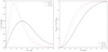 |
Fig. 4. Same as Fig. 3, for viewing angle. Distributions are normalized. |
| In the text | |
|
Fig. 5. Left: mean viewing angle of jointly detected events, as function of horizon and radio sensitivity s. Values of H for O2, O3 and design instruments, as well as s for VLA, SKA1 and SKA2/ngVLA, are indicated as dashed lines. Right: fraction of on-axis events (defined by θv ≤ θj) among jointly detected events in same H–s diagram. |
| In the text | |
|
Fig. 6. Left: cumulative distributions of peak times of radio afterglows for jointly detected events in O3-VLA configuration, assuming jet with (solid line) or without (dashed line) lateral expansion. Middle: differential distribution of peak fluxes of GW-detected events assuming horizon for O2 (dotted line), O3 (dashed line) and design (full line) configurations of GW interferometers. The radio sensitivities for VLA, SKA1 and SKA2/ngVLA are indicated for comparison. Right: differential distribution of maximum proper motion for jointly detected events assuming O2-VLA (dotted line), O3-VLA (dashed line), design-SKA1 (full line) configurations. The dotted vertical line shows the lower limit for detection of the proper motion. |
| In the text | |
|
Fig. 7. Predicted samples of GW-detected (dots) and jointly detected (crosses) mergers in planes of various pairs of observables, for O3-VLA configuration. Upper left: distance and viewing angle, and maximum distance at which the proper motion can be measured (Dmax(θv), see Eq. (18), green dotted line). Upper right: peak flux and viewing angle. Lower left: time of radio afterglow peak (assuming lateral expansion of jet) and viewing angle. Lower right: maximum remnant proper motion and distance, and limiting proper motion μlim (green dotted line). |
| In the text | |
|
Fig. 8. Differential distribution of core jet kinetic energy (left) and external medium density (right) of entire GW population (full) and jointly detected events (dashed), in O3-VLA configuration. Distributions are normalized to fraction of jointly detected events among all GW-detected events, see text for details. |
| In the text | |
|
Fig. 9. Left: fraction of joint events among GW events assuming short GRB luminosity function from Wanderman & Piran (2015) for different values of minimum kinetic energy Em (full lines), and for our fiducial model (dashed lines), in O3-VLA configuration. Results have been plotted for different values of the jet opening angle θj = 0.05, 0.1 and 0.15 rad (red, black and blue lines respectively). Middle: mean viewing angle (same color coding). Right: fraction of joint events with peaks earlier than 150 days post-merger, with hypothesis of jet lateral expansion, same color coding. |
| In the text | |
Current usage metrics show cumulative count of Article Views (full-text article views including HTML views, PDF and ePub downloads, according to the available data) and Abstracts Views on Vision4Press platform.
Data correspond to usage on the plateform after 2015. The current usage metrics is available 48-96 hours after online publication and is updated daily on week days.
Initial download of the metrics may take a while.