| Issue |
A&A
Volume 630, October 2019
|
|
|---|---|---|
| Article Number | A117 | |
| Number of page(s) | 12 | |
| Section | Numerical methods and codes | |
| DOI | https://doi.org/10.1051/0004-6361/201935973 | |
| Published online | 01 October 2019 | |
Incorporating astrochemistry into molecular line modelling via emulation
1
Department of Physics and Astronomy, University College London, Gower Street, London WC1E 6BT, UK
e-mail: ucapdde@ucl.ac.uk
2
Department of Statistical Science, University College London, Gower Street, London WC1E 6BT, UK
Received:
23
May
2019
Accepted:
5
July
2019
In studies of the interstellar medium in galaxies, radiative transfer models of molecular emission are useful for relating molecular line observations back to the physical conditions of the gas they trace. However, doing this requires solving a highly degenerate inverse problem. In order to alleviate these degeneracies, the abundances derived from astrochemical models can be converted into column densities and fed into radiative transfer models. This ensures that the molecular gas composition used by the radiative transfer models is chemically realistic. However, because of the complexity and long running time of astrochemical models, it can be difficult to incorporate chemical models into the radiative transfer framework. In this paper, we introduce a statistical emulator of the UCLCHEM astrochemical model, built using neural networks. We then illustrate, through examples of parameter estimations, how such an emulator can be applied to real and synthetic observations.
Key words: astrochemistry / radiative transfer / methods: statistical / ISM: molecules / galaxies: abundances
© ESO 2019
1. Introduction
Molecules form in the interstellar medium provided it is dense enough for collisions to bring the chemical reactants together, and cool enough to suppress the complete dissociation of chemical products. Observations of the interstellar medium in and outside of our galaxy have revealed a rich and diverse chemistry (Shematovich 2012), spanning a wide range of physical environments. As stars form through the collapse of over-densities inside this optically opaque dense interstellar medium (Young & Scoville 1991), the study of molecular gas can provide a window into the star-formation process and shed light onto the life cycle of galaxies.
Typically, the chemistry of the cold and dense interstellar medium is probed through measurements of molecular lines. In order to interpret these, radiative transfer models are used to relate the line strengths back to the physical conditions of the interstellar medium they trace. RADEX (see van der Tak et al. 2007) is a popular non-local thermodynamic equilibrium (non-LTE) radiative transfer model that models, for a given set of physical conditions, the expected strength of molecular lines. By matching the observed molecular lines to predictions from grids of such models, it is possible to constrain the density, temperature, and column density of the molecular gas (e.g. Viti 2017; Tunnard & Greve 2016; Salak et al. 2018).
However, as molecular line intensities are dependent on a complex interplay between the physics, chemistry, and radiative transfer of the observed region, their interpretation is often ambiguous. As such, estimating chemical parameters via the use of radiative transfer models is a notoriously degenerate problem. Even under a set of idealized assumptions, when one assumes that the gas can be accurately represented using a single component at a unique temperature and density, there exist wide ranges of parameter values capable of fitting a set of observations (see Tunnard & Greve 2016; Kamenetzky et al. 2018). These degeneracies are amplified when studying external galaxies as the telescope beam sizes often encompass a wide variety of different physical environments that must be disentangled.
Since line intensity predictions obtained from radiative transfer models depend on the column densities of the studied region, it is customary to treat column densities as free parameters of the radiative transfer modelling to be constrained alongside the temperature and density. Unfortunately, this makes the radiative transfer modelling highly degenerate, oftentimes leading to many very different models being able to fit the same observations. There have been attempts to address these degeneracies through the use of astrochemical models.
Astrochemical models, such as UCLCHEM presented in Holdship et al. (2017), are computational codes designed for modelling the chemical composition of gas under well-defined physical conditions. This is done through the numerical integration of a set of differential equations constructed from a network of chemical reactions. It has been proposed, for example in Viti et al. (2014) and more recently in Viti (2017) and Harada et al. (2019), to convert the outputs of chemical models into column densities to be used as inputs to radiative transfer models. Without including chemistry into the forward model, parameter retrieval can give retrievals that are inconsistent with our current knowledge of chemistry as the forward model has no knowledge of which species should be abundant for a given set of conditions. With inclusion of the chemistry, not only are column densities no longer free parameters, leading to tighter bounds on the retrieved parameters, but it becomes possible to constrain the parameters driving the chemistry, such as for example the metallicity and cosmic-ray ionization rate. However, the widespread integration of astrochemical models into the radiative transfer process is hindered by their long running times and their complexity. The long running times result in even a relatively small grid of astrochemical models requiring a large amount of computational resources.
In this project, we address both of these issues through the creation of a publicly available statistical emulator for the UCLCHEM astrochemical model1. The statistical emulator is built using a set of neural networks trained to find a multidimensional fit to a training dataset of chemical simulations. The emulator offers a considerable speed-up in modelling time, being able to estimate molecular abundances in milliseconds, much faster than full chemical models which run in minutes. In addition to the speed-up, the UCLCHEM emulator has been simplified, now being dependent on only six variables: density, temperature, metallicity, visual extinction, cosmic-ray rate, and radiation field rate of the region being modelled. With our emulator, the complexity and computational power required to include chemical models into the radiative transfer process has been considerably reduced. As a by-product, we have also created a RADEX emulator for a select few key species for an even faster inference.
Although emulators have gained some traction in the cosmology community (e.g. Schmit & Pritchard 2018; Kwan et al. 2015), they remain uncommon in astrochemistry. The astrochemical community instead usually favours comparison to tables of precomputed models (e.g. Mondal et al. 2019; Meijerink et al. 2007; Maffucci et al. 2018; Bisbas et al. 2019). In Grassi et al. (2011), a neural network was trained to replace the chemical network calls in N-body simulations. Our work differs in that, by modelling the full chemical evolution starting from a limited set of realistic initial conditions, we have restricted the parameter space. This avoids issues of error propagation over each time-step and allows the use of more complex chemical models.
In Sect. 2, we give some details on the physical and chemical models being emulated as well as the emulation procedure. In Sects. 3 and 4, we give a technical overview of our emulation procedure and quantify, over our selected parameter range, the ability of our emulator to accurately predict molecular abundances and intensities. In Sect. 5, using a set of toy observations, we demonstrate how the emulator can help to lift some of the degeneracies present in radiative transfer modelling. In Sect. 6, we further apply the emulators to ALMA observations of the nearby prototypical Seyfert 2 galaxy NGC 1068 (presented in García-Burillo et al. 2014; Viti et al. 2014) and touch upon some of the weaknesses and strengths of our emulator.
2. Modelling molecular gas
In this section we give a brief overview of the specifics of the chemical and radiative transfer models used for emulation. We explain how we combined these to create a simple forward model capable of reproducing observations of the interstellar medium. We finish the section by covering how we can use a neural network to create an emulator of astronomical models.
2.1. Chemical models
UCLCHEM is a time-dependent gas-grain open-source chemical model described in Holdship et al. (2017). In UCLCHEM, chemical evolution of the gas is divided into two phases. In the first phase (phase I), supposed to approximate the molecular gas formation processes, the gas starts in a diffuse atomic state and evolves following a freefall collapse. In the second phase of the model (phase II), the physical conditions are modified so as to approximate specific observable environments. For an extragalactic application, this could involve high cosmic-ray rates as would be expected in an AGN-dominated galaxy, or high UV flux as would be expected in a starburst galaxy.
For our models, during phase I the gas started at a density of 100 cm−3 and was then compressed via freefall to a final density, which was left as a free parameter. This freefall collapse was isothermal, with a gas temperature of 10 K. The radius of the region, which was also used to calculate the visual extinction, was allowed to vary. During this phase, gas phase desorption and freeze-out on the dust grains proceeds.
During phase II, the gas was assumed to have reached its final density and the physical parameters were varied so as to model a range of environments. The models were all run for 107 years, long enough for the gas to reach chemical equilibrium. The parameters that were allowed to vary were the following.
-
Temperature (T): The temperatures of the phase II models were increased over time up to a value T following the same procedure as in Viti et al. (2004), where the temperature increases with time as a function of the luminosity of an evolving star. Indeed, the temperature dependence on time will differ depending on which objects the chemical model is simulating, but for the purpose of this study we simply adopted the procedure already present in UCLCHEM. The models were then further run at fixed temperatures until a cumulative time of 107 years.
-
Gas density (n): The phase I models were run following a parametric freefall collapse (Rawlings et al. 1992) until a density n was reached. The density was then kept constant during phase II.
-
Metallicity (mZ): The initial atomic abundances used by the chemical network were constrained to be a fraction of the solar metallicity. We defined metallicity as a multiplicative factor with a metallicity of 1 corresponding to elemental abundances as found in Asplund et al. (2009).
-
Cosmic-ray ionization rate (ζ): This parameter represented the cosmic-ray ionization rate used in Phase II. Additionally, as we do not model the X-ray ionization rate, we use the cosmic-ray ionization rate as its proxy (Xu & Bai 2016). As noted in Viti et al. (2014) this approximation has its limitations in that X-ray heating is more efficient than cosmic-ray heating.
-
Ultraviolet-photoionization rate (χ): This parameter represented the UV-photoionization rate used for phase II models. The UV-photoionization is measured in Draine where 1 Draine is equivalent to 1.6 × 10⁻³ erg s−1 cm−2 (Draine 1978; Draine & Bertoldi 1996).
-
Visual extinction (AV): In UCLCHEM the visual extinction of the molecular gas is controlled by the size of the modelled region.
At its core, the UCLCHEM chemical model is centred around a chemical network specified by the user. For this project we used a chemical network based on the UMIST database (McElroy et al. 2013). For each time-step, a set of coupled ordinary differential equations is generated from the chemical network and solved. We refer the reader to the UCLCHEM release paper (Holdship et al. 2017) for a thorough overview of the effect of various parameters on these rate equations.
2.2. The radiative transfer model
The non-LTE radiative transfer code RADEX (van der Tak et al. 2007) in conjunction with collision files obtained from the LAMBDA database (Schöier et al. 2005) was used for estimating line intensities. RADEX is a non-LTE radiative transfer model that decouples the non-local radiation field from the local-level population calculation through the escape probability approximation.
For our emulator, all radiative transfer models were run with H2 as the unique collisional partner, assuming a background temperature of 2.7 K and assuming a spherical geometry. As both Krips et al. (2011) and Viti et al. (2014) found that different geometry choices in RADEX gave comparable outputs for the fitting of CO, HCN, and HCO+ in a nearby galaxy we restrict ourselves to using a spherical geometry.
2.3. The forward model
Using molecular line intensities to constrain the physical conditions of the interstellar medium is an inverse problem. In practice, this can be tackled by comparing synthetic line-intensity predictions obtained using a forward model with the measured molecular lines. In this paper we contrast two distinct forward-modelling approaches:
-
The forward model can encompass solely the radiative transfer physics (from now on referred to as chemistry-independent). This is the more established methodology for analysing molecular lines (Imanishi et al. 2018; Michiyama et al. 2018).
-
The forward model can alternatively encompass the chemistry of the molecular gas in addition to the radiative transfer (from now on referred to as chemistry-dependent). This approach is less common but has been used in Harada et al. (2019), Viti (2017), and Viti et al. (2014).
In the chemistry-independent forward-modelling approach, the temperature, gas density, line-width, column-densities, and beam-filling factor are the only parameters allowed to vary. The first four parameters correspond to the input parameters used in the RADEX modelling. The beam-filling factor is treated as a multiplicative scaling factor.
In the chemistry-dependent forward model, the parameters allowed to vary are the inputs to the chemical model, the line widths, and the beam-filling factor. In this case the synthetic observations are created by converting the output abundances from the chemical model into column densities and using these, as well as the final chemical model temperature and density, as inputs to the radiative transfer model. The predicted intensities from the radiative transfer model are then transformed into mock observations by multiplying them by a beam-filling factor. In order to convert abundances into column densities, the fractional abundances are multiplied by the column densities of hydrogen as measured at 1 mag and by the visual extinction. We used N(H2) = 1.6 × 1021 cm−3 for the column density of hydrogen at 1 mag. This conversion procedure is known as the “on-the-spot” approximation (e.g. Dyson & Williams 1997).
These models can easily be extended to include more than one phase of gas. For example, for a two-phase gas, one can run two single-phase models and add up their intensities (after rescaling by the beam-filling factor). A summary of the newly introduced parameters and their notation is as follows:
-
The line width (Δv): This is the line width used as an input in the RADEX radiative transfer calculations. For simplicity, we assume in our forward model that all molecular lines share a common line width.
-
The filling factor (f): For each phase, the output intensities from RADEX are rescaled by a beam-filling factor representing the fraction of the beam occupied by the emission.
2.4. Artificial neural networks
Artificial neural networks (ANNs) are a class of algorithms used for learning mappings between an input space and an output space (Goodfellow et al. 2016), and are trained by tuning a set of parameters to match a training dataset composed of input–output pairs. The building blocks of ANNs are nodes, called neurons, connected together by edges. In an ANN, information is passed between nodes through these edges and combined through non-linear functions to obtain a mapping from the input to the output space.
In feed-forward neural networks (Fig. 1), as used in this project, the neurons are organized into sequential layers. The neurons from each layer are connected by edges to every neuron of the succeeding and preceding layer. Neurons are place-holders in which numbers are stored with the first layer containing the inputs fed to the neural network and the last layer containing the associated predictions from the neural network. All the neurons in other layers are place-holders for intermediate values used in the calculations. The predicted outputs, given an input, are found by successively calculating for each layer the values of the neurons, starting from the input layer up to the output layer. For neuron j, the formula for calculating its value aj is aj = Φ(∑iwijai + bj) where ∑i refers to a sum over all the neurons of the previous layer, bj is a parameter associated to every individual neuron usually referred to as “bias”, and wij is a parameter associated to every individual edge and is referred to as the “weight of the edge”. The function Φ(x), often called the activation function, is a non-linear function whose presence makes it possible to approximate non-linear combinations of the inputs. For this specific project a rectified linear unit (ReLU) activation function was used (Vinod & Hinton 2010).
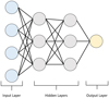 |
Fig. 1. Illustration of a multilayer perceptron neural network. |
The neural network parameters (bias and weights) are determined using a set of training data. Typically, the training data contain example inputs and their associated outputs. The neural network then attempts to fine-tune the parameters so as to minimize a user-specified loss function, designed to assess how well the neural network predictions match the example outputs.
In this project we utilize neural networks as emulators. This consists of using the inputs of a model as the inputs to a neural network and training the neural network to reproduce the outputs of the model. By training a neural network to emulate a model, it becomes possible to bypass the model. This is advantageous if the model is computationally intensive to run, as it allows samples to be obtained at a fraction of the original computational cost.
In the application presented here, because there is a strong overlap in the parameter space explored when modelling different galaxy observations, very similar grids of parameters are run even when interpreting radically different observations. This makes the use of an emulator particularly advantageous as the overhead required in training an emulator will quickly be smaller than the accumulated run-time from running redundant models.
3. UCLCHEM emulator
In this section we discuss the creation and evaluation of our emulator.
3.1. The training dataset
A dataset of N = 120 000 chemical models was generated. The parameter ranges for the training dataset can found in Table 1. Since the emulator is only able to interpolate and not extrapolate, these parameter ranges define the usable range of the emulator.
Emulator parameters and their range.
A Latin hypercube sampling scheme was used for generating the samples in the training dataset. Latin hypercube sampling (McKay et al. 1979) is a statistical method for generating near random samples, which is particularly suitable for exploring parameter spaces under a restricted computational budget. It has been used, for example, in Schmit & Pritchard (2018) for the emulation of the epoch of reionization simulations and in Bower et al. (2010) for emulation of semi-analytical galaxy models.
3.2. The algorithm
Feed-forward neural networks were used to predict molecular log-abundances from the UCLCHEM inputs. A separate neural network was trained for each molecular species in our chemical network with each neural network sharing the same five-layer architecture. The first layer was six neurons wide, with each neuron being assigned to one of the six input parameters. The next three layers were successive hidden layers of width 200, 100, and 50. Finally the last layer represented the predicted output by the neural network. All of the layers used a ReLU activation function (Vinod & Hinton 2010).
For each molecular species, the neural network was trained through the backpropagation algorithm (see Rumelhart et al. 1986) to minimize the MSE loss over the whole dataset between the chemical simulation outputs and the neural network outputs
with yi being the log10-abundance predicted by UCLCHEM, xi the neural network input parameters (see Table 1), and  the neural network prediction. As abundances cover several orders of magnitude in scale, in order to treat the whole parameter range equally we trained the neural network to minimize the log-abundances. In addition, the input parameters were scaled to lie within a range from zero to one before being fed to the neural network by using the following transform:
where X is an input parameter before rescaling.
Training of the neural networks was done using the pytorch framework (Paszke et al. 2017). The neural network parameters were optimized using Adam (Kingma & Ba 2015) with an initial learning rate of 0.001 and training occurring over 20 epochs, with batches of 500 in size.
3.3. Error analysis
We quantified the approximation error in our emulation procedure by plotting the distribution of differences between the emulated log-abundances and the UCLCHEM log-abundances for a validation dataset, constructed by running 10 000 UCLCHEM models with randomly sampled input parameters (Fig. 2). Reassuringly, the emulation error is small for all of our plotted species, with 95% of the models agreeing with the emulator predictions to within a multiplicative factor of 1.13 (a log10-abundance difference of 0.05). At the tail of the distribution, the worst emulator predictions are still within a factor of ten of the correct abundances (a log10-abundance difference of 1).
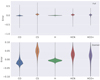 |
Fig. 2. Violin plot of the distribution of the difference between the log10 abundance predictions from the astrochemical models and those from the emulator using a kernel density estimate from the 10 000 simulations in the validation dataset for CO, CS, H, HCN, and HCO+. Bottom plot: zoomed-in version of the top plot. Bottom plot: thick black lines represent the interquartile range and the thin black line the 95% confidence interval. |
3.4. Effect of the dataset size
We investigated the effect the training dataset size had on the predictive power of our emulator. To do this, we trained our neural networks on differently sized subsets of the training dataset and quantified how the training dataset size affected predictions. For each dataset size, we averaged the validation set errors over multiple runs. The outcome is shown in Fig. 3, where we can see that further increasing the dataset size beyond the 120 000 samples already used would only offer very marginal improvements to the predictive ability of our emulator.
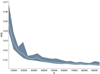 |
Fig. 3. Effect of training set size on emulator prediction. The y-axis shows the mean squared error between the log10 ground truth abundances and neural network prediction evaluated on the validation dataset. The x-axis shows the size of the training dataset. The shaded area represents the spread of mean squared error obtained across runs; the 68.2% percentiles centered around the mean are shaded. |
4. Radiative transfer emulator
In addition to creating an emulator for UCLCHEM, we created a radiative transfer emulator that replicated the results obtained by RADEX for J < 10 molecular line transitions. As each molecule required a brand new set of RADEX models to be run, we restricted ourselves to emulating HCO+, HCN, CO, and CS. Although individual RADEX models are relatively quick to run, exploring a high-dimensional radiative transfer parameter space can require hundreds of thousands of simulations. This makes the use of a RADEX emulator particularly useful, especially in cases where a slight loss in accuracy is acceptable, such as when used in conjunction with chemical models, which themselves have high associated uncertainties.
4.1. Training dataset
The emulator took the temperature, density, line-width, and molecular column densities as inputs. By exploiting the degeneracy between line width and column density for optical depth, we were able to remove the line-width dependency from our training dataset. All the parameter ranges were kept the same as for the UCLCHEM emulator, with the maximal column densities for our RADEX emulator rounded up to be an order of magnitude larger than the maximal column densities in our chemical model dataset. A Latin hypercube sampling scheme was run over the chosen parameter range. We sampled from the log-column density.
The escape-probability formalism that underpins RADEX can break down for some parameter choices, leading to spurious intensities. To mitigate this effect we applied a visually chosen cut-off to the intensities in our training-set; all simulations with intensities higher than the cutoff were excluded from the dataset.
4.2. Algorithm
We used the same neural network preprocessing, training, and architecture as that used for the UCLCHEM emulator. We trained the neural network using an L1 loss:
with yi referring to the intensity predicted by RADEX, xi the corresponding RADEX input parameters, and  the neural network prediction on a dataset of approximately 100 000 RADEX outputs. Because our method for removing spurious intensities was not perfect, there remained some spurious models. This meant that an L1 loss, which put less emphasis on fitting every single data point perfectly, was more suitable then an L2 loss. To prevent the neural network from predicting nonphysical values, we rounded all negative intensity predictions to zero.
To assess our emulators effectiveness we plotted the difference between RADEX and our emulator alongside the distribution of RADEX intensities for comparison, for a dataset of 10 000 unseen RADEX simulations for CO, CS, HCO+ and HCN (Figs. 4 and 5). From these figures, we can see that the errors in molecular intensity associated to using the RADEX emulator are comparatively small compared to the errors associated to using the UCLCHEM emulators. In addition, as it is unlikely that all unphysical RADEX simulations have been removed, the tails of our violin plot may be skewed from the unphysical models. From this, we see that the uncertainties associated to the RADEX emulator should be much smaller than those associated to the UCLCHEM emulator. As such, the RADEX emulator should have a minimal impact on our predictions. However, we caution that this situation would change if we were modelling multiple line transitions as, because of the shared column density, the uncertainty from the RADEX emulator would then have a much greater impact.
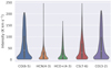 |
Fig. 4. Violin plot of the distribution of RADEX intensities for different molecular lines. The distributions are obtained using a kernel density estimate from the 10 000 simulations in the dataset. The thick black lines represent the interquartile range and the thin black lines the 95% confidence intervals. |
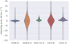 |
Fig. 5. Violin plot of the distribution of the difference between intensity predictions from the emulator and from RADEX for different molecular lines. The distribution is obtained using a kernel density estimate from the 10 000 simulations in the dataset. |
5. Bayesian posterior evaluation
In this paper we advocate the use of emulators as a computationally efficient way of incorporating chemical models into the estimation of model parameters.
To assess the benefits obtained from the inclusion of a chemical model in the forward model, we contrast parameter estimation with and without chemical models. The parameter estimation was performed using Bayesian statistics. The PyMultinest implementation of the Nested Sampling algorithm (see Skilling 2006; Feroz et al. 2009; Buchner et al. 2014) was used for sampling from our posterior probability distributions.
In the following sections we begin by giving a brief overview of the Bayesian formalism. We then cover, using increasingly complex models, the advantages and disadvantages of the parameter estimation using our chemical emulator.
We wish to emphasize that in the following sections our objective is to highlight how the emulator may be used for parameter estimation. There is some level of flexibility in how the likelihood may be parametrized, and we do not claim that the parametrization we used is necessarily optimal.
5.1. Bayesian formalism
Given a model governed by a set of parameters, Bayesian statistics make it possible to mathematically quantify the effect previously unseen data has on further focusing the parameters. In this framework, a probability distribution is associated to each parameter. The prior probability distribution reflects the belief of the user in terms of the parameters before accounting for data. This probability distribution will be high in regions of the parameter space likely to coincide with the true parameters and low in other regions. The posterior probability distribution represents the updated probability distribution after accounting for observations; it is mathematically related to the prior distribution through Bayes rule:
where P(θ ∣ d) is the posterior distribution and P(θ) is the prior distribution. P(d ∣ θ) is defined as the likelihood; it describes how plausible the obtained data is given a set of parameters. The denominator is referred to as the “evidence”. In this project, because the data are kept constant, the evidence behaves as a normalization constant and can be ignored.
5.2. Application
In this section we describe how we applied the Bayesian statistical formalism towards constraining physical parameters from observations of molecular lines. We consider the case where we have observed N molecular line transitions obtaining observations

with xi being the intensity of the ith molecular species. Here, we also consider that we wish to estimate p(θ ∣ X) with θ a vector describing the molecular gas parameters of a forward model f. Using Bayes Rule we can express this in terms of the likelihood and the prior distribution. For our purposes, we consider that our observations correspond to the intensities predicted from our forward model with an independent additive Gaussian noise. This leads to a log-likelihood of the form
with A being a normalization constant, σi the uncertainty associated to the ith species, and f(θ) the vector of intensities predicted by the forward model f for model parameters θ. The forward model can either be chemistry-independent or chemistry-dependent (see Sect. 2.3).
We set uniform or log-uniform priors on all the parameters with ranges matching the emulator range. The choice of uniform prior meant that all values within the prior bounds were expected to be equally likely, while the choice of log-uniform priors meant that all scales within the bounds were expected to be equally likely. Uniform priors were used for the temperature, visual extinction, line width, filling factor, and metallicity. Log-uniform priors were used for the cosmic-ray ionization rate, UV-photoionization rate, number density, and scaled column densities. Unless otherwise stated, we used parameter priors as found in Table 2.
Default prior distributions on model parameters.
5.3. Posterior evaluation
It can be prohibitively expensive to evaluate a high-dimensional posterior distribution. This motivates the use of efficient parameter-space exploration techniques which prioritize resource allocation towards exploring high-probability regions of parameter space. Because of the multimodality found in some of our posterior distributions, we used the pymultinest Python module (Buchner et al. 2014) to evaluate our posterior distributions; this is a python wrapper for the multinest package (Feroz et al. 2009) which is itself an implementation of the nested sampling algorithm (Skilling 2006). We used the corner module (Foreman-Mackey 2016) to visualize the marginalized posterior parameter distributions.
5.4. One-phase model
5.4.1. Generation
So as to contrast and evaluate the two forward-modelling approaches, we generated a set of synthetic observations using the nonemulated UCLCHEM and RADEX. The parameters used for generating the observations can be found in Table 3 and the resultant intensities can be found in Table 4. In this case we assumed a known beam-filling factor of f = 1.
Parameters used for creating the single-phase model.
Intensities (K km s−1) of the single-phase model.
5.4.2. Posterior estimation
We attempted to retrieve the parameters using the chemistry dependent forward model and the chemistry independent forward model. In both cases, we assumed observational uncertainties of 20% and prior distributions as defined in Table 2. Marginalized one- and two-dimensional posterior probability distributions for the temperature, density, and line width, as obtained using the corner module, are shown in Fig. 6 for the chemistry-independent forward model and in Fig. 7 for the chemistry-dependent forward model. For the chemistry-independent forward model, the posterior distribution was evaluated using the emulated models, while for the chemistry-dependent forward model, the posterior distribution was evaluated using both the emulated (black) and nonemulated model (blue).
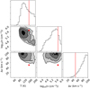 |
Fig. 6. Marginalised posterior distributions obtained when using a single-phase “chemistry-independent” forward model. The true parameters, plotted in red, can be found in Table 3. |
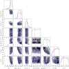 |
Fig. 7. Marginalized posterior distributions obtained when using a single-phase chemistry dependent forward model. The posterior distributions obtained using the emulators are plotted in black while those obtained using the nonemulated models are plotted in blue. The true parameters, plotted in red, can be found in Table 3. |
We see that the posterior distributions obtained using the emulated and nonemulated forward models (Fig. 7) are in excellent agreement with each other. This further supports our findings from previous sections that the emulator can reproduce the RADEX and UCLCHEM model predictions with high fidelity.
From these figures, it is apparent that the chemistry-dependent and the chemistry-independent parameter estimations give very different predictions. While the chemistry-independent parameter estimation struggles to constrain the temperature and density of the molecular gas, the chemistry-dependent estimation is able to return tight and accurate confidence bounds on the parameters.
5.5. Two-phase model
5.5.1. Generation
To further test our parameter retrieval process, we modeled a new molecular gas phase by generating an additional set of intensities, approximating a lower temperature molecular phase, using the nonemulated UCLCHEM and RADEX. We then modeled a beam containing two molecular gas phases by adding the two phases after scaling them by beam-filling factors. The parameters used for generating the two phases and the intensities of the two phases can be found in Tables 5 and 6. These parameters roughly correspond to a beam filled with one hot and dense phase and one cool and diffuse phase.
Parameters used for creating the two-phase model.
Intensities (K km s−1) of the two-phase model.
5.5.2. Posterior estimation
Much like in the previous section, we next attempted to fit our two-phase observations using chemistry-dependent and chemistry-independent forward models. In both cases, we used the emulated two-phase forward models with prior distributions identical to those used in the single-phase forward models (Table 2) on both phases and assumed uncertainties of 20% on the observations (Viti et al. 2014). As we set both prior distributions to cover the full emulated range, the forward model could hypothetically fit the observations with two hot-gas phases or two cold-gas phases. This is in contrast with what has sometimes been done, such as in Tunnard et al. (2015), where the authors constrained the two phases to nonoverlapping parameter ranges, thus artificially forcing the gas to exist in two very distinct phases. In this analysis we have forced the two phases of gas to share the same metallicity and line width.
The marginalized posterior distributions obtained are plotted in Figs. 8 and 9. Once again, we see that both approaches give very different constraints on the posterior probability distributions. Although both methods arguably struggle to retrieve the correct temperature and density, the chemistry-dependent forward-model predictions occupy a more narrow range of the parameter space.
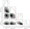 |
Fig. 8. Marginalized posterior distributions obtained when using a two-phase chemistry-independent forward model. The true parameters, plotted in green and red, can be found in Table 5. |
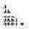 |
Fig. 9. Marginalized posterior distributions obtained when using a two-phase chemistry-dependent forward model. The true parameters, plotted in green and red, can be found in Table 5. |
In addition, the chemistry-dependent forward model also partially recovers the two-phase bimodality. Even though this is most apparent in the plot of filling factor against density, it is also visible in the temperature-versus-density plot. The above results collectively indicate that the chemistry-dependent estimation is capable, at least partially, of picking out the two distinct phases of gas, even when the chemistry-independent forward model struggles to constrain any of the parameters. On the other hand, we see that our parameter estimation underestimates the line width.
6. Application to real line ratios
In the previous section, we used synthetic observations to assess the benefits brought by incorporating chemistry into radiative transfer forward models. However, although synthetic observations are useful in that they offer a controllable and well-understood test bed, there are aspects of working with real regions that cannot be easily understood with synthetic observations. Below is an inexhaustive list of these complications.
-
Even though in recent years there has been tremendous progress towards understanding the chemistry in the interstellar medium (Williams & Viti 2013), there are still significant uncertainties associated to the reactions therein. Because of these, the chemistry in our forward model may not accurately match that occurring in real regions.
-
Is only usable for the parameter range under which it was trained (Table 1).
-
The molecular abundances predicted by our emulator are those reached after the chemical models have been run long enough for an equilibrium to be reached. As such, any transient chemical variation will not be captured by our emulator.
-
For molecular observations, and particularly for observations with large beam sizes, the approximation that the gas can be represented using a small number of components is likely to break down.
For the reasons highlighted above, we thought it important to showcase the performance of the emulator on real observations. To do this, we used ALMA observations of NGC 1068, a prototypical nearby Seyfert barred galaxy as presented in Viti et al. (2014) and Viti (2017). This galaxy is believed to host a rich chemical diversity and as such it is expected to be very difficult to disentangle the chemistry occurring within. We focused on the spectral lines measured in the East Knot, a region of the molecular ring showing strong emission, and used the degraded resolution measurements as presented in the original paper (Viti et al. 2014); the measured intensities have been retranscribed and can be found in Table 8. Although we have every reason to believe that the molecular gas spans a wide range of physical conditions, to avoid using an excessively complex forward model, we fit the region using a single-phase molecular component.
After running an exploratory single-phase chemistry-dependent parameter estimation, we found that our models were consistently unable to reproduce the HCO+ intensities. To further investigate this issue, we evaluated the HCO+(4–3)/CO(3–2) line-intensity ratio for all of the UCLCHEM models used by our emulator. We found that all of the chemical models in our training dataset resulted in line-intensity ratios smaller than the ratio observed with ALMA. This suggests that our models, over the parameter range studied, does not produce enough HCO+ to match the observations.
This was in itself not surprising, as chemical models have been known to struggle with producing enough HCO+ to match observations (e.g. Godard et al. 2010; Viti et al. 2014). In Papadopoulos (2007), it was argued that because of the sensitivity of the HCO+ column density to the ionization degree of the molecular gas, HCO+ can be an unreliable tracer of hot dense gas. Furthermore, if the HCO+ is a transient species or if it is created in low-visual-extinction and high-density clumps not covered by our emulation, then it is likely that our models would not capture it.
In light of our inability to reproduce HCO+ observations, we reran a parameter estimation identical in all but the fact that HCO+ was excluded from the fitting. The posterior plots obtained without HCO+ can be found in Fig. 10. From this we can see that the Bayesian parameter estimation, for fitting a single phase, favors a component with moderately high temperature (T ∼ 120 K) but very high density (n ∼ 106 cm−3).
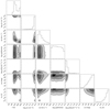 |
Fig. 10. Marginalized posterior distributions obtained when using a single-phase chemistry-dependent forward model on the ALMA observations excluding HCO+. |
It is informative to quantify the goodness of fits of some of the models from the posterior distributions. We show, for a small representative sample of well-fit models, the model parameters in Table 7 and the corresponding intensities in Table 8. From these tables, it becomes clear that the intensities predicted by the emulated and nonemulated forward model are in excellent agreement. These tables also highlight the strong degeneracies which exist in the forward modeling process.
Example input model parameters.
Of note is that the HCN intensity recovered by the Bayesian parameter estimation, although at the correct order of magnitude, was consistently lower than the observed HCN intensity. Almost none of the best-fitting models predicted an HCN intensity greater than the observed intensity. This could be interpreted as the models struggling to create a high enough HCN intensity which could be indicative that the molecular phase, not captured by our models, which is responsible for the high HCO+ intensity may also be at least partially responsible for a portion of the HCN intensity.
7. Conclusions
In this paper we propose an alternative method for interpreting the physical conditions of the interstellar medium from the analysis of molecular line intensities. This is typically approached by running many forward models and finding the input parameters to the non-LTE radiative transfer forward model whose predictions match well with observations.
By feeding the outputs of a chemical model into the RADEX radiative transfer model, as was expanded upon in Sect. 2.3, it is possible to re-parametrize the radiative transfer forward model. In this formalism, the forward-model dependency on column densities is replaced with a dependency on physical parameters. This offers the potential to lift parameter degeneracies. However, the subsequent forward model is not computationally practical as the required chemical models are computationally expensive to run at scale.
We present and evaluate an emulator, created using neural networks, capable of predicting molecular abundances at a fraction of the run-time of the UCLCHEM astrochemical model, as well as an emulator approximating the outputs of the RADEX radiative transfer codes. We show that by using our emulators it becomes computationally tractable to run the chemistry-dependent forward models accurately at scale.
By applying our emulator to mock observations as well as real observations we show that incorporating chemistry into the parameter retrieval cannot only lead to tighter constraints on the retrieved physical parameters but also constrain parameters introduced by the chemical models such as the cosmic-ray ionization rate and metallicity. We also show that our emulator-based approach is able to distinguish between two distinct phases of molecular gas where a traditional radiative transfer approach fails.
Finally, by applying our formalism to real observations of the galaxy NGC 1068, we show that our emulator can effectively be applied to obtain information from real observations. This comes with the caveat that the emulator may struggle to reproduce certain molecular lines such as the HCO+ molecular lines. However, we argue that this inability to reproduce HCO+ may be indicative of molecular gas with extreme physical conditions not within our emulation range.
We would like to conclude this paper by emphasizing that we have had to make choices in defining the likelihood for our experiments, but that these choices may not be optimal. For example, the likelihood could be designed to not only put emphasis on having the line intensities at the correct scale, as was done in our experiments, but also to put emphasis on preserving the relative strength of lines tracing the same species. Finally, the likelihood could also be designed to put stronger constraints on species for which the chemical modeling has been benchmarked and well understood. Furthermore, in most applications it is probably sensible to further constrain or fix some of the forward model parameters, such as the metallicity.
Emulator can be found at github.com/drd13/emulchem
Acknowledgments
DDM is supported by the STFC UCL Centre for Doctoral Training in Data Intensive Science (grant number ST/P006736/1). The authors also acknowledge DiRAC for use of their HPC system which allowed this work to be performed. The authors would also like to thank the referee Tommaso Grassi for helpful comments.
References
- Asplund, M., Grevesse, N., Sauval, A. J., & Scott, P. 2009, Annu. Rev. Astron. Astrophys., 47, 481 [CrossRef] [Google Scholar]
- Bisbas, T. G., Schruba, A., & van Dishoeck, E. F. 2019, MNRAS, 485, 3097 [NASA ADS] [Google Scholar]
- Bower, R. G., Vernon, I., Goldstein, M., et al. 2010, MNRAS, 407, 2017 [NASA ADS] [CrossRef] [Google Scholar]
- Buchner, J., Georgakakis, A., Nandra, K., et al. 2014, A&A, 564, A125 [NASA ADS] [CrossRef] [EDP Sciences] [Google Scholar]
- Draine, B. T. 1978, ApJS, 36, 595 [NASA ADS] [CrossRef] [Google Scholar]
- Draine, B. T., & Bertoldi, F. 1996, ApJ, 468, 269 [NASA ADS] [CrossRef] [EDP Sciences] [Google Scholar]
- Dyson, J. E. J. E., & Williams, D. A. 1997, The Physics of the Interstellar Medium (Institute of Physics Pub), 165 [Google Scholar]
- Feroz, F., Hobson, M. P., & Bridges, M. 2009, MNRAS, 398, 1601 [NASA ADS] [CrossRef] [Google Scholar]
- Foreman-Mackey, D. 2016, J. Open Source Softw., 1, 24 [Google Scholar]
- García-Burillo, S., Combes, F., Usero, A., et al. 2014, A&A, 567, A125 [NASA ADS] [CrossRef] [EDP Sciences] [Google Scholar]
- Godard, B., Falgarone, E., Gerin, M., Hily-Blant, P., & De Luca, M. 2010, A&A, 520, A20 [NASA ADS] [CrossRef] [EDP Sciences] [Google Scholar]
- Goodfellow, I., Bengio, Y., & Courville, A. 2016, Deep Learning (The MIT Press) [Google Scholar]
- Grassi, T., Merlin, E., Piovan, L., Buonomo, U., & Chiosi, C. 2011, ArXiv e-prints [arXiv:1103.0509] [Google Scholar]
- Harada, N., Nishimura, Y., Watanabe, Y., et al. 2019, ApJ, 871, 238 [NASA ADS] [CrossRef] [Google Scholar]
- Holdship, J., Viti, S., Jiménez-Serra, I., Makrymallis, A., & Priestley, F. 2017, AJ, 154, 38 [NASA ADS] [CrossRef] [Google Scholar]
- Imanishi, M., Nakanishi, K., & Izumi, T. 2018, ApJ, 856, 143 [NASA ADS] [CrossRef] [Google Scholar]
- Kamenetzky, J., Privon, G. C., & Narayanan, D. 2018, ApJ, 859, 9 [NASA ADS] [CrossRef] [Google Scholar]
- Kingma, D. P., & Ba, J. 2015, 3rd International Conference on Learning Representations, ICLR 2015, San Diego, CA, USA, May 7–9, 2015, Conference Track Proceedings [Google Scholar]
- Krips, M., Martín, S., Eckart, A., et al. 2011, ApJ, 736, 37 [NASA ADS] [CrossRef] [Google Scholar]
- Kwan, J., Heitmann, K., Habib, S., et al. 2015, ApJ, 810, 35 [NASA ADS] [CrossRef] [Google Scholar]
- Maffucci, D. M., Wenger, T. V., Gal, R. L., & Herbst, E. 2018, ApJ, 868, 41 [NASA ADS] [CrossRef] [Google Scholar]
- McElroy, D., Walsh, C., Markwick, A. J., et al. 2013, A&A, 550, A36 [NASA ADS] [CrossRef] [EDP Sciences] [Google Scholar]
- McKay, M. D., Beckman, R. J., & Conover, W. J. 1979, Technometrics, 21, 239 [Google Scholar]
- Meijerink, R., Spaans, M., & Israel, F. P. 2007, A&A, 461, 793 [NASA ADS] [CrossRef] [EDP Sciences] [Google Scholar]
- Michiyama, T., Iono, D., Sliwa, K., et al. 2018, ApJ, 868, 95 [NASA ADS] [CrossRef] [Google Scholar]
- Mondal, A., Das, R., Shaw, G., & Mondal, S. 2019, MNRAS, 483, 4884 [NASA ADS] [CrossRef] [Google Scholar]
- Papadopoulos, P. P. 2007, ApJ, 656, 792 [NASA ADS] [CrossRef] [Google Scholar]
- Paszke, A., Gross, S., Chintala, S., et al. 2017, NIPS Autodiff Workshop [Google Scholar]
- Rawlings, J. M. C., Hartquist, T. W., Menten, K. M., & Williams, D. A. 1992, MNRAS, 255, 471 [NASA ADS] [CrossRef] [Google Scholar]
- Rumelhart, D. E., Hinton, G. E., & Williams, R. J. 1986, Nature, 323, 533 [NASA ADS] [CrossRef] [PubMed] [Google Scholar]
- Salak, D., Tomiyasu, Y., Nakai, N., et al. 2018, ApJ, 856, 97 [NASA ADS] [CrossRef] [Google Scholar]
- Schmit, C. J., & Pritchard, J. R. 2018, MNRAS, 475, 1213 [NASA ADS] [CrossRef] [Google Scholar]
- Schöier, F. L., van der Tak, F. F. S., van Dishoeck, E. F., & Black, J. H. 2005, A&A, 432, 369 [NASA ADS] [CrossRef] [EDP Sciences] [Google Scholar]
- Shematovich, V. I. 2012, Sol. Syst. Res., 46, 391 [NASA ADS] [CrossRef] [Google Scholar]
- Skilling, J. 2006, Bayesian Anal., 1, 833 [CrossRef] [MathSciNet] [Google Scholar]
- Tunnard, R., & Greve, T. R. 2016, ApJ, 819, 161 [NASA ADS] [CrossRef] [Google Scholar]
- Tunnard, R., Greve, T. R., Garcia-Burillo, S., et al. 2015, ApJ, 815, 114 [NASA ADS] [CrossRef] [Google Scholar]
- van der Tak, F. F. S., Black, J. H., Schöier, F. L., Jansen, D. J., & van Dishoeck, E. F. 2007, A&A, 468, 627 [NASA ADS] [CrossRef] [EDP Sciences] [Google Scholar]
- Vinod, N., & Hinton, G. 2010, Proceedings of the 27th International Conference on International Conference on Machine Learning (Association for Computing Machinery), 170 [Google Scholar]
- Viti, S. 2017, A&A, 607, A118 [Google Scholar]
- Viti, S., Collings, M. P., Dever, J. W., McCoustra, M. R. S., & Williams, D. A. 2004, MNRAS, 354, 1141 [NASA ADS] [CrossRef] [Google Scholar]
- Viti, S., García-Burillo, S., Fuente, A., et al. 2014, A&A, 570, A28 [NASA ADS] [CrossRef] [EDP Sciences] [Google Scholar]
- Williams, D. A., & Viti, S. 2013, Observational Molecular Astronomy: Exploring the Universe Using Molecular Line Emissions (Cambridge University Press) [CrossRef] [Google Scholar]
- Xu, R., & Bai, X.-N. 2016, ApJ, 819, 68 [NASA ADS] [CrossRef] [Google Scholar]
- Young, J. S., & Scoville, N. Z. 1991, Annu. Rev. Astron. Astrophys., 29, 581 [Google Scholar]
All Tables
All Figures
|
Fig. 1. Illustration of a multilayer perceptron neural network. |
| In the text | |
|
Fig. 2. Violin plot of the distribution of the difference between the log10 abundance predictions from the astrochemical models and those from the emulator using a kernel density estimate from the 10 000 simulations in the validation dataset for CO, CS, H, HCN, and HCO+. Bottom plot: zoomed-in version of the top plot. Bottom plot: thick black lines represent the interquartile range and the thin black line the 95% confidence interval. |
| In the text | |
|
Fig. 3. Effect of training set size on emulator prediction. The y-axis shows the mean squared error between the log10 ground truth abundances and neural network prediction evaluated on the validation dataset. The x-axis shows the size of the training dataset. The shaded area represents the spread of mean squared error obtained across runs; the 68.2% percentiles centered around the mean are shaded. |
| In the text | |
|
Fig. 4. Violin plot of the distribution of RADEX intensities for different molecular lines. The distributions are obtained using a kernel density estimate from the 10 000 simulations in the dataset. The thick black lines represent the interquartile range and the thin black lines the 95% confidence intervals. |
| In the text | |
|
Fig. 5. Violin plot of the distribution of the difference between intensity predictions from the emulator and from RADEX for different molecular lines. The distribution is obtained using a kernel density estimate from the 10 000 simulations in the dataset. |
| In the text | |
|
Fig. 6. Marginalised posterior distributions obtained when using a single-phase “chemistry-independent” forward model. The true parameters, plotted in red, can be found in Table 3. |
| In the text | |
|
Fig. 7. Marginalized posterior distributions obtained when using a single-phase chemistry dependent forward model. The posterior distributions obtained using the emulators are plotted in black while those obtained using the nonemulated models are plotted in blue. The true parameters, plotted in red, can be found in Table 3. |
| In the text | |
|
Fig. 8. Marginalized posterior distributions obtained when using a two-phase chemistry-independent forward model. The true parameters, plotted in green and red, can be found in Table 5. |
| In the text | |
|
Fig. 9. Marginalized posterior distributions obtained when using a two-phase chemistry-dependent forward model. The true parameters, plotted in green and red, can be found in Table 5. |
| In the text | |
|
Fig. 10. Marginalized posterior distributions obtained when using a single-phase chemistry-dependent forward model on the ALMA observations excluding HCO+. |
| In the text | |
Current usage metrics show cumulative count of Article Views (full-text article views including HTML views, PDF and ePub downloads, according to the available data) and Abstracts Views on Vision4Press platform.
Data correspond to usage on the plateform after 2015. The current usage metrics is available 48-96 hours after online publication and is updated daily on week days.
Initial download of the metrics may take a while.