| Issue |
A&A
Volume 630, October 2019
|
|
|---|---|---|
| Article Number | A125 | |
| Number of page(s) | 12 | |
| Section | Galactic structure, stellar clusters and populations | |
| DOI | https://doi.org/10.1051/0004-6361/201935886 | |
| Published online | 03 October 2019 | |
He abundances in disc galaxies
I. Predictions from cosmological chemodynamical simulations
1
School of Physics and Astronomy, University of Birmingham, Edgbaston B15 2TT, UK
e-mail: This email address is being protected from spambots. You need JavaScript enabled to view it.
2
Centre for Astrophysics Research, University of Hertfordshire, College Lane, Hatfield AL10 9AB, UK
Received:
14
May
2019
Accepted:
24
July
2019
Abstract
We investigate how the stellar and gas-phase He abundances evolve as a function of time within simulated star-forming disc galaxies with different star formation histories. We make use of a cosmological chemodynamical simulation for galaxy formation and evolution, which includes star formation as well as energy and chemical enrichment feedback from asymptotic giant branch stars, core-collapse supernovae, and Type Ia supernovae. The predicted relations between the He mass fraction, Y, and the metallicity, Z, in the interstellar medium of our simulated disc galaxies depend on the galaxy star formation history. In particular, dY/dZ is not constant and evolves as a function of time, depending on the specific chemical element that we choose to trace Z; in particular, dY/dXO and dY/dXC increase as a function of time, whereas dY/dXN decreases. In the gas-phase, we find negative radial gradients of Y, due to the inside-out growth of our simulated galaxy discs as a function of time; this gives rise to longer chemical enrichment timescales in the outer galaxy regions, where we find lower average values for Y and Z. Finally, by means of chemical-evolution models, in the galactic bulge and inner disc, we predict steeper Y vs. age relations at high Z than in the outer galaxy regions. We conclude that for calibrating the assumed Y − Z relation in stellar models, C, N, and C+N are better proxies for the metallicity than O because they show steeper and less scattered relations.
Key words: galaxies: abundances / galaxies: evolution / ISM: abundances / stars: abundances / hydrodynamics
© ESO 2019
1. Introduction
In order to study the star formation history (SFH) of our Galaxy, undestanding how He abundances are distributed in the stars and interstellar medium (ISM) is fundamental for a precise estimate of stellar ages for different metallicity and star-formation environments (Iben 1968; Chiosi & Matteucci 1982; Fields 1996; Chiappini et al. 2002; Jimenez et al. 2003; Romano et al. 2007). Stellar ages in our Galaxy are typically inferred either by fitting the observed colour–magnitude diagram (CMD) with a set of stellar isochrones (e.g. Bensby et al. 2014), or by adding asteroseismic constraints (Casagrande et al. 2016; Silva Aguirre & Serenelli 2016; Miglio et al. 2017; Silva Aguirre et al. 2018). In both cases the resulting age distributions rely on the assumptions and underlying physics of stellar models (Casagrande et al. 2007; Lebreton et al. 2014). One of the most important assumptions of stellar models is given by the initial He content of the stars, and stellar models are usually calibrated assuming a linear scaling relation between the He mass fraction, Y⋆ = MHe/M⋆, and the stellar metallicity, Z⋆ (which may be obtained from absorption lines in stellar spectra; e.g. Pagel & Portinari 1998).
Historically, helium abundances in the stars of our Galaxy could only be directly measured in the photospheres of O- and B-type stars (Struve 1928; Shipman & Strom 1970; Morel et al. 2006; Nieva & Przybilla 2012), because in the later spectral types there are no strong He absorption features for accurate spectroscopic analysis. Helium abundances in the ISM of galaxies can be directly measured within Galactic and extragalactic HII regions by making use of optical He recombination lines (e.g. HeI λ4471, λ5875; see, e.g. Peimbert et al. 2017); in metal-poor HII regions, these observations have been instrumental in determining (via extrapolation towards zero metallicity) an independent estimate of the primordial He abundance to compare with the predictions of Big Bang nucleosynthesis (e.g. Peimbert & Torres-Peimbert 1976; Peimbert et al. 2002; Luridiana et al. 2003; Olive & Skillman 2004; Izotov et al. 2007; Valerdi et al. 2019). Another viable means of measuring He abundances in the HII regions uses the He radio recombination lines in the 8–10 GHz frequency interval (Balser 2006). Finally, He abundance measurements can also be obtained in planetary nebulae (e.g. Pottasch & Bernard-Salas 2010; Stanghellini et al. 2006) and in absorptions systems along the line of sight to quasars at high redshift (Cooke & Fumagalli 2018).
It is interesting to note that Aver et al. (2015) showed that the HeI λ10830 emission line in the near-infrared – when combined with high-quality optical data – can be used to greatly reduce the uncertainties in the abundance analysis; HeI λ10830 is strongly sensitive to the HII region electron density (Izotov et al. 2014), and this can be used to break the density–temperature degeneracy in the abundance analysis.
Putting together the results of all studies, one finds large variations for dY/dZ, ranging in the interval [1.5, 2.5]1. This makes the best calibration for Y = Y(Z, t) assumed in stellar models highly uncertain, from both an observational and theoretical point of view (e.g. Casagrande et al. 2007; Portinari et al. 2010; Gennaro et al. 2010); in turn, this results in a large uncertainty in the final estimate of stellar ages. In particular, the impact of assumed dY/dZ may give rise to relative variations in the measurement of stellar ages from asteroseismic analysis as high as ∼40 % (Lebreton et al. 2014; Miglio et al., in prep.). Moreover, Nataf & Gould (2012) pointed out that there may be critical issues in determining the ages of Galactic bulge stars if dY/dZ ≠ const. (see also Renzini et al. 2018).
It is therefore important to investigate how the He content in the ISM and in the stars of galaxies depends on the metallicity and SFH. In this paper, we present the first attempt to study how He is produced and then released by ageing stellar populations in galaxies, making use of a state-of-the-art cosmological chemodynamical simulation (Vincenzo & Kobayashi 2018a,b).
Our paper is structured as follows. In Sect. 2, we summarise the main characteristics of our cosmological hydrodynamical simulation. In Sect. 3, we describe how He is deposited by ageing stellar populations of different metallicities in our simulation, and try to quantify the uncertainty due to different stellar yield assumptions by means of a one-zone chemical-evolution model. In Sect. 4, we present the results of our study on He in the ISM and in the stars of our simulated galaxies. Finally, in Sect. 5, we draw our conclusions.
2. Assumed cosmological simulation
In this paper we make use of the same cosmological hydrodynamical simulation code as described in detail in Kobayashi et al. (2007) and Vincenzo & Kobayashi (2018a,b), which is based on the GADGET-3 code (Springel 2005). Our simulation code includes star formation activity with mass- and metallicity-dependent chemical and thermal energetic feedback from (i) stellar winds of dying asymptotic giant branch (AGB) and massive stars of all masses and metallicities, (ii) Type Ia supernovae (SNe Ia), and (iii) Type II SNe (SNe II) and hypernovae (HNe).
We assume the same nucleosynthesis prescriptions as in Kobayashi et al. (2011), modified to include failed SNe for masses m ≥ 25 M⊙ and metallicities Z ≥ 0.02 of the progenitor massive stars (see also Smartt 2009; Müller et al. 2016; Beasor & Davies 2018; Prantzos et al. 2018; Limongi & Chieffi 2018; Sukhbold & Adams 2019; Kobayashi et al., in prep.). Finally, the initial mass function (IMF) is that of Kroupa (2008, similar to Chabrier 2003), defined between 0.01 and 120 M⊙.
In our simulation, we evolve a cubic volume of the Λ-cold dark matter (ΛCDM) Universe, with the cosmological parameters being given by the nine-year Wilkinson Microwave Anisotropy Probe (Hinshaw et al. 2013). We assume periodic boundary conditions and a box side ℓU = 10 Mpc h−1, in comoving units. We have a total number of gas and DM particles which is NDM = Ngas = 1283, with the following mass resolutions: MDM ≈ 3.097 × 10⁷ h−1 M⊙ and Mgas = 6.09 × 10⁶ h−1 M⊙. Finally, the gravitational softening length is ϵgas ≈ 0.84 h−1 kpc in comoving units. Our simulations are in good agreement with the observed cosmic SFR, mass-metallicity relations, and the N/O–O/H relation (Vincenzo & Kobayashi 2018b).
2.1. Three reference galaxies
In this paper, we investigate how He abundances vary within three simulated disc galaxies, selected from the ten reference galaxies of Vincenzo & Kobayashi (2018b). In particular, our galaxy A corresponds to galaxy 3 of Vincenzo & Kobayashi (2018b), galaxy B to galaxy 6, and galaxy C to galaxy 9. Nevertheless, our results for He would have been the same had we selected other galaxies from Vincenzo & Kobayashi (2018b) 2.
In Fig. 1 we show the age distribution of the stellar populations in galaxies A−C as predicted at the present time. The different curves in Fig. 1 are normalised such that the area below each of them corresponds to the total galaxy stellar mass at redshift z = 0. It is clear from the figure that – from galaxy A to galaxy C – the SFH becomes more and more concentrated towards later epochs of cosmic time.
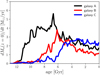 |
Fig. 1. Predicted age distribution of the stellar populations in our three reference galaxies. The curves are such that the area below each of them corresponds to the galaxy stellar mass at redshift z = 0. |
In summary, our three reference galaxies at redshift z = 0 have the following total stellar and gas masses: (i) M⋆,A = 3.29 × 10¹⁰ M⊙ and Mgas,A = 1.10 × 10¹⁰ M⊙; (ii) M⋆,B = 1.60 × 10¹⁰ M⊙ and Mgas,B = 1.21 × 10¹⁰ M⊙; (iii) M⋆,C = 1.55 × 10¹⁰ M⊙ and Mgas,C = 1.79 × 10¹⁰ M⊙.
3. He nucleosynthesis in the simulation
Apart from the primordial nucleosynthesis, which accounts for most of the He in the Universe, He can be synthesised and released into the ISM of galaxies by stars of all mass ranges with m⋆ ≳ 1 M⊙. The main source of uncertainty for the He nucleosynthesis in our cosmological simulation is given (i) by the assumptions about stellar rotation and mass loss in massive star models (see the review by Maeder 2009), and (ii) by the treatment of overshooting, convective boundary conditions, hot-bottom burning, and efficiency of the third dredge-up (mixing processes) in AGB stellar models (see the detailed discussion in Ventura et al. 2013; Renzini 2015; Karakas & Lugaro 2016; Karakas et al. 2018).
In Fig. 2, we show how the average IMF-weighted stellar yields of He, ⟨𝒫He⟩, vary as a function of initial stellar metallicity, Z⋆, by assuming some different stellar models for massive and AGB stars. In particular, the quantity ⟨𝒫He⟩ is computed as follows:
 (1)
(1)
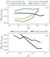 |
Fig. 2. (a) Average IMF-weighted stellar yield of He from massive stars as a function of the initial stellar metallicity, as predicted by the stellar models of Nomoto et al. (2013, black solid line) and Limongi & Chieffi (2018) for different stellar rotational velocities; in particular, the blue, green, and orange lines correspond to the Limongi & Chieffi (2018) stellar models with vrot = 0, 150, and 300 km s−1, respectively. (b) Average IMF-weighted stellar yield of He from AGB stars as a function of initial stellar metallicity, as predicted by the stellar models of Karakas (2010, black solid line) and Ventura et al. (2013, blue solid line). |
for massive stars, where pHe(m, Z⋆) represents the He stellar yield as a function of mass and metallicity, and
 (2)
(2)
for AGB stars.
In Fig. 2a, the average stellar yields of He from the massive star models of Nomoto et al. (2013) – which include mass loss and SN nucleosynthesis but not the effect of rotation – are compared with the average yields of Limongi & Chieffi (2018), which include also the effect of rotation. In particular, the different curves in Fig. 2a for the Limongi & Chieffi (2018) yields correspond to models with different stellar rotational velocities (v0, v150, and v300, which stand for vrot = 0, 150, and 300 km s−1, respectively). At subsolar metallicities, massive star models with increasingly high rotational velocities give rise – on average – to increasingly small amounts of He; moreover, the stellar yields of He from rotating stellar models show a stronger dependence on metallicity than non-rotating massive star models; as we see in Sect. 3.2, these resulting differences in the stellar yields for massive stars give rise to a systematic uncertainty in the predictions of chemical evolution models.
Finally, in Fig. 2b, the average stellar yields of He from the AGB stellar models of Ventura et al. (2013) are compared with those of Karakas (2010) assumed in our cosmological simulation. We find that the Karakas (2010) stellar yield of He decreases as a function of metallicity, and this makes the Ventura et al. (2013) stellar yield larger by a factor of approximately two at solar and super-solar metallicities. The most important differences between the two stellar models reside in the physics of super-adiabatic convection and mixing (Karakas et al. 2002; Karakas & Lattanzio 2007), which affect the final stellar yield from AGB stars.
3.1. Production rate of He from simple stellar populations of different metallicity in our cosmological simulation
In order to understand how He is produced by the stars in our simulation, in Fig. 3, we show how much He is deposited by simple stellar populations (SSPs) of different metallicity, per unit time and per unit mass of the SSPs (namely, in units of  , where MSSP represents the initial mass of the SSP), by assuming the same stellar lifetimes and IMF as in our cosmological simulation. We note that each star particle in our simulation is treated as a SSP (Kobayashi 2004).
The contribution from massive stars and AGB stars to the He chemical enrichment is highlighted in Fig. 3; in particular, we compare our results with the Nomoto et al. (2013) stellar yields for massive stars (coloured curves) with the stellar yields of Limongi & Chieffi (2018, grey shaded area) for rotating massive stars. There is a tendency for more metal-rich AGB stars to release slightly larger amounts of He into the ISM per unit time. We note that the gap in the figure around 30–50 Myr (blue shaded horizontal region) corresponds to stellar masses in the range between 8 and 10 M⊙ (even though this mass range is quite uncertain), which are not included in most galactic chemical-evolution models including ours. Nevertheless, super-AGB stars do not provide a significant contribution to the global chemical enrichment of galaxies (see, e.g. Vangioni et al. 2018; Prantzos et al. 2018; Kobayashi et al., in prep.).
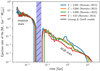 |
Fig. 3. Predicted ejection rate of He from stellar populations of different metallicities (different colours) by assuming the stellar yields of Nomoto et al. (2013). The grey shaded area corresponds to our predictions when assuming the Limongi & Chieffi (2018) set of stellar yields of rotating massive stars with different metallicities ([Fe/H] = 0, −1, −2, and −3 dex) and stellar rotational velocities (vrot = 0, 150, and 300 km s−1). The blue shaded horizontal region corresponds to the chemical enrichment of super-AGB stars which are not included in our galactic chemical evolution model. |
We provide a useful formalism to compute the He production rate from a SSP of age t and metallicity Z, by firstly defining a partial yield per stellar generation as follows:
 (3)
(3)
where pHe represents the stellar nucleosynthetic yield of He from all the stars with mass m and metallicity Z in the SSP, as weighted with the assumed IMF, mmax corresponds to the maximum stellar mass which is formed in the SSP, and mTO(t, Z) represents the turn-off mass (as computed from the inverse stellar lifetimes). The extremes of the integral in Eq. (3) enclose all the stars that, at the time t from the birth time of the SSP, have already died, enriching the galaxy ISM with He.
The production rate of He by a SSP with metallicity Z and age t can then be computed as follows:
 (4)
(4)
which is the quantity shown on the y-axis of Fig. 3.
3.2. Quantifying the systematic uncertainty in the predicted Y–Z relation due to different sets of stellar yields
To understand the effect of different stellar yield assumptions for massive stars and AGB stars on the Y vs. Z relation in galaxies, in Fig. 4 we show the predictions of different one-zone chemical evolution models, assuming a star formation efficiency (SFE) of 2.0 Gyr−1, infall time-scale τinf = 4.0 Gyr, and no galactic wind. The models are developed assuming that the galaxy assembles by accreting a total amount of gas Minf ≈ 3.16 × 10¹¹ M⊙ with primordial chemical composition. The accretion of gas into the galaxy potential well follows the following law: ℐ(t) ∝ e−t/τinf. Finally, for the SFR, we assume a linear Schmidt-Kennicutt relation, namely SFR(t) = SFE × Mgas(t).
In Fig. 4a,c, we fix the stellar yields of AGB stars and vary the stellar yields of massive stars. In particular, for AGB stars, in Fig. 4a we fix the stellar yields of Karakas (2010), whereas in Fig. 4c we fix the stellar yields of Ventura et al. (2013). The stellar yields of massive stars that we explore in Figs. 4a,c are those of Nomoto et al. (2013) and those of Limongi & Chieffi (2018) for different rotational velocities (v = 0, 150, and 300 km s−1) and iron abundances ([Fe/H] = 0, −1, −2, and −3 dex) of the progenitor massive star. Finally, in Figs. 4b,d, we fix the stellar yields of massive stars, and we explore the effect of varying the stellar yields of AGB stars assuming the yields of Karakas (2010) and Ventura et al. (2013). In particular, in Fig. 4b, we fix the massive star yields of Limongi & Chieffi (2018), whereas in Fig. 4d we fix those of Nomoto et al. (2013).
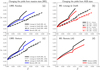 |
Fig. 4. Effect of different nucleosynthesis yields for massive stars (panels a and c) and AGB stars (panels b and d) on the predicted Y vs. Z relation from a one-zone galaxy chemical evolution model with star formation efficiency SFE = 2 Gyr−1, infall timescale τ = 4 Gyr, and no galactic winds. For massive stars we explore the stellar yields of Nomoto et al. (2013), which are adopted in our cosmological simulations, and the stellar yields of Limongi & Chieffi (2018) for different stellar rotational velocities (v0, v150 and v300 represent rotational velocity v = 0, 150, and 300 km s−1, respectively). For AGB stars, we explore the stellar yields of Karakas (2010), adopted in our cosmological simulations, and those of Ventura et al. (2013); see also e.g. Vincenzo et al. (2016). |
We find that the uncertainty on the predicted Y vs. Z relation due to different stellar yield assumptions for massive stars increases as a function of metallicity, being ΔYMS(0 < Z ≲ 0.01) ∼ 0.004; at super-solar metallicities, where stellar yields are more uncertain, we find ΔYMS(Z > 0.01) ∼ 0.008. If we fix the stellar yields of massive stars and vary the nucleosynthetic assumptions for AGB stars, we find an uncertainty that again increases with metallicity, being ΔYAGB(0 < Z ≲ 0.01) ∼ 0.002 and ΔYAGB(Z > 0.01) ∼ 0.0065, giving rise to an uncertainty in the predicted dY/dZ due to different stellar yield assumptions for AGB stars, which can be as large as ≈0.35.
4. Results
In this section we present the results of our analysis for the evolution of the He abundances in our simulated disc galaxies. In Sect. 4.1 we focus on the He abundances within the ISM, comparing the predictions of our simulation with the observed He abundances in metal-poor HII regions by Aver et al. (2015) and Fernández et al. (2019), whereas in Sect. 4.3 we study the He content in the stellar populations. Finally, in Sect. 4.4 we compare the predictions of our simulation with He abundance measurements in a Galactic open cluster (McKeever et al. 2019), horizontal branch stars in Galactic globular clusters (Mucciarelli et al. 2014), RR Lyrae stars in the Galactic bulge (Marconi & Minniti 2018), and in a sample of B-type stars in our Galaxy (Morel et al. 2006; Nieva & Przybilla 2012).
4.1. He abundances in the ISM
The ISM abundances of He in our simulated galaxies are explored in Fig. 5. In the lower right corner of each panel, we report our best fits to the predicted Y − XO, Y − XC, Y − XN, and Y − XC+N relations in our three reference galaxies, assuming a simple linear law. First of all, as we consider galaxies with SFHs concentrated towards later and later epochs (namely, by moving from galaxy A to galaxy C), we note that the slopes of Y − XO and Y − XC diminish, whereas the slope of Y − XN increases. Secondly, the spread in Y − XC, N is much smaller than that in Y − XO.
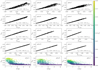 |
Fig. 5. First row (top): gas-phase He mass fraction, Ygas, as a function of the gas-phase O mass fraction, XO,gas. Second row: Ygas vs. XC,gas. Third row: Ygas vs. XN,gas. Fourth row: Ygas vs. XC+N,gas. Fifth row (bottom): predictions for the radial profile of Ygas as a function of the galactocentric distance, d, with the colour coding representing the O mass fraction. From left to right, the various columns correspond to each of our reference galaxies, from galaxy A to galaxy C, respectively. |
The lower scatter in Y − XC, N is a consequence of the fact that the absolute abundances of C and N are much lower than those of O; in particular, we obtain the following approximate value for the relative abundance variations of i= C, N, O, and C+N in our three simulated galaxies, for He abundances in the range [0.27, 0.29]:
 (5)
(5)
Our findings suggest that the calibration of the Y − Z relation for stellar models should be carried out using nitrogen or carbon abundances; however, since C and N abundances at the stellar surface may be strongly affected by (extra)mixing (e.g. Iben & Renzini 1983; Shetrone et al. 2019), we suggest to use C+N, which is instead a conserved quantity at the stellar surface, as the stars experience dredge-up episodes after they leave the main sequence.
We predict radial gradients of both Y and XO in the ISM of our simulated galaxies (see the bottom panels of Fig. 5); in particular, we find that the most central galaxy regions have higher average metallicites and also higher He abundances than the outermost regions. To reach those high ISM metallicities in the central regions, numerous generations of stars should have succeeded each other polluting the ISM with metals and He, giving rise to very short chemical enrichment timescales in the galaxy centre. In fact, we find that our simulated disc galaxies grow from the inside out (see also Vincenzo & Kobayashi 2018b), giving rise to chemical enrichment timescales which increase as a function of galactocentric distance, d; this in turn determines the predicted trend of Y and Z as a function of d.
In Fig. 6 we show how our best-fit values for dY/dXO, dY/dXC, dY/dXN, dY/dXC+N, and dY/dZ in the ISM of our three reference galaxies evolve as a function of look-back time, where Z represents the sum of the abundances of all 31 chemical elements contributing to metallicity, which are traced in our simulation. We only show our predictions for the epochs when the total galaxy stellar mass is >5 × 10⁹ M⊙, in order to have a sufficient number of resolution elements for each galaxy. It is clear from the figure that galaxies with different SFHs also exhibit different temporal evolution of dY/dXC,N,O. Interestingly, the temporal evolution of dY/dXN shows an opposite trend with respect to that of dY/dXO, dY/dXC, and dY/dZ.
On the one hand, we predict that dY/dXN diminishes as a function of time; this is due to the fact that N is mostly produced as a secondary element, and its stellar yields steadily increase with metallicity, whereas the He stellar yields have a weaker dependence on metallicity than those of N. This way, the variation in N between two consecutive time-steps is always larger than that of He, at any epoch of the galaxy evolution.
On the other hand, dY/dXO increases with time, because – in the declining phase of the galaxy SFH – the variation of He between two consecutive time-steps is larger than that of O; this is due to the large production of He from AGB stars of all masses and metallicities, which pollute the ISM over a large range of delay times from the star formation event. Finally, the evolution of dY/dXC is weaker than that of dY/dXO and dY/dXN, because He and C are strictly coupled from the point of view of the stellar nucleosynthesis. Interestingly, the evolution with time of dY/dXC+N, as well as its dependence on the galaxy SFH, is relatively weak, varying from ∼6.4 to 6.6.
Our predicted values for dY/dXO in Fig. 6 are consistent with the He abundance measurements in extragalactic HII regions, which use O lines to estimate the ISM metallicity, finding dY/dXO ∼ 2.2−2.4 (Izotov et al. 2007). Alternatively, our predicted values for dY/dZ are lower than those determined with indirect He abundance measurements in Galactic open clusters, which report dY/dZ ∼ 1.4 (Brogaard et al. 2012).
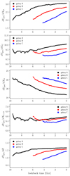 |
Fig. 6. Predicted evolution of dYgas/dXO (top panel), dYgas/dXC (second panel), dYgas/dXN (third panel), dYgas/dXC+N (third panel), and dYgas/dZ (bottom panel) as a function of look-back time. The black, red, and blue curves correspond to galaxies A, B, and C, respectively. The values of dYgas/dXC,N,O,Z correspond to our best-fit values for the predicted Ygas − XC,N,O,Z relations in each galaxy, by assuming a simple linear law at all times. We only show the evolution of the slopes for times when the galaxy stellar mass M⋆ > 5 × 10⁹ M⊙. |
The offset between model and data for dY/dZ could be due to the systematic uncertainty in the He nucleosynthesis from AGB stars. For example, by assuming the Ventura et al. (2013) stellar yields, there is a more pronounced He enrichment at high metallicities from AGB stars, giving rise to steeper Y − Z relations (i.e. higher dY/dZ) than those predicted with the Karakas (2010) stellar yields (see Fig. 4). Nevertheless, various studies in the past estimated dY/dZ ∼ 2.1 for relatively large samples of stars in our Galaxy (Jimenez et al. 2003; Casagrande et al. 2007; Portinari et al. 2010), corresponding to a value which is much larger than that found in Galactic open clusters by Brogaard et al. (2012). There is therefore some uncertainty also on the observational side on the value of dY/dZ, mostly because of the indirect methods employed to determine the He content of the stars, which are strongly dependent on the assumptions of stellar evolution models (e.g. Portinari et al. 2010).
4.2. Redshift evolution of the He/H abundances in the ISM
Figures 7a–c show the predicted redshift evolution of the gas-phase He/H vs. O/H abundance pattern in our three simulated disc galaxies. For comparison, we also show the He/H abundance measurements as determined in the HII regions of a sample of 16 metal-poor dwarf irregular galaxies in the local Universe by Aver et al. (2015); the black triangles with error bars correspond to the final qualifying sample of Aver et al. (2015), whereas the grey triangles with error bars correspond to their flagged HII region abundances, which are affected by large systematic uncertainties. Finally, in the same figure, we also show the He/H abundance measurements of Fernández et al. (2019, magenta triangles with error bars) for a sample of young metal-poor HII regions (see also Fernández et al. 2018, for more information about their galaxy sample), who employed a Bayesian approach to fit the spectra in the abundance analysis determination.
At fixed O/H abundances, we predict that He/H steadily increases as a function of time; this increase in He/H is faster as we move towards higher metallicities, which typically correspond to the more central galaxy regions. This is due to the fact that the most central galaxy regions had the highest star formation activity in the past, giving rise to an enhancement of the He abundances in those regions at the present time. Moreover, the SFR in our simulated disc galaxies propagates from the inside out (see also Vincenzo & Kobayashi 2018b), being stronger at the beginning in the galaxy central regions, and reaching the outer disc over longer typical timescales; this explains why fixed He/H abundances are reached at later times, if their corresponding O/H abundances are lower.
We note that the observed data in Figs. 7a–c correspond to abundances within different metal-poor emission-line galaxies, which are put all together in the figure, whereas our simulation data correspond to abundance variations in the ISM of a single disc galaxy. Nevertheless, the observations show much more scatter at low metallicity than our simulated disc galaxies, which are characterised – in their low-metallicity outskirts – by very homogeneous He/H abundances of ≈0.08, approximately corresponding to the assumed primordial He/H ratio in the simulation.
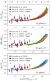 |
Fig. 7. Redshift evolution of the gas-phase He/H−O/H abundance pattern in our three simulated disc galaxies. The blue points correspond to the predicted gas-phase abundances at redshift z = 0, orange points to z = 0.5, green points to z = 1, and red points to z = 2. The black and grey triangles with error bars correspond to the observational data of Aver et al. (2015) for a sample of metal-poor HII regions within 16 emission-line galaxies in the Local Universe; the black triangles correspond to their qualifying sample, whereas the grey triangles mark the abundances affected by large systematic uncertainty. Finally, the magenta points with error bars correspond to the observational data of Fernández et al. (2019). |
The difference in the scatter at low metallicity between the observations and our simulation may be due to the fact that in the outskirts of our simulated galaxies we do not see strong star formation activity; on the other hand, in the observed galaxy samples of Aver et al. (2015) and Fernández et al. (2019) there are prominent Hα lines, which are the signature of ongoing star formation activity. These relatively high SFRs at low metallicities may explain such variation in He/H in the observed data. Nevertheless, we highlight the fact that the mass-resolution of our simulation is ≈ 106 M⊙ for primordial gas particles; therefore, at low metallicity, the pollution of He from a single star formation episode with low intensity would be distributed to a large number of ∼106 M⊙ surrounding gas particles, all with primordial He/H ratio, giving rise to more homogeneous abundances at low metallicity. Finally, the observed scatter at low metallicity may be the signature of He enrichment from rotating massive Wolf–Rayet stars (Kumari et al. 2018), which are not included in our cosmological simulation.
To demonstrate that the gas fraction is one of the main parameters driving the evolution of the average He abundances in our simulated disc galaxies, in Fig. 8 we show how the average SFR-weighted He/H abundances in the ISM of our three simulated disc galaxies evolve as a function of the galaxy gas fraction, which is defined as fgas = Mgas/(Mgas + M⋆). As the galaxy evolves, because of the continuous star-formation activity, fgas decreases as a function of time. At the same time, we predict that the average He/H abundances in the gas-phase increase, with He being produced by a larger number of ageing stellar populations in the galaxy.
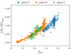 |
Fig. 8. Evolution of the average SFR-weighted He/H abundance as a function of the gas fraction (fgas = Mgas/(Mgas + M⋆)) within our simulated disc galaxies. Blue points correspond to galaxy A, orange points to galaxy B, and green points to galaxy C. |
Finally, in Fig. 9, we show how the inclusion of failed SNe affects the predicted He/H vs. O/H abundance patterns at redshift z = 0 in our reference simulated galaxies. Our findings are very similar to those presented in Vincenzo & Kobayashi (2018a) for the N/O vs. O/H abundance pattern; in particular, we find that the inclusion of failed SNe increases the inhomogeneity of the chemical abundance patterns, making also the final galaxies less metal-rich at the present time. The assumption of failed SNe changes the evolution of the metallicity as a function of time by shifting the stellar metallicity distribution function towards lower metallicities; this way, there is – on average – a larger production of He as a function of time (see also Fig. 2, which shows that AGB stars with higher metallicities eject – on average – lower amounts of He per unit time). Therefore, at fixed O/H abundances, the simulation with failed SNe predicts higher He/H abundances in the galaxy ISM.
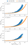 |
Fig. 9. Predicted gas-phase He/H−O/H abundance pattern at redshift z = 0 in our three simulated disc galaxies, by assuming failed SNe (blue points), like in our reference cosmological hydrodynamical simulation, and by running a similar simulation without failed SNe (orange points). |
4.3. He abundances in the stellar populations
In Fig. 10 we investigate how the He abundances in the stars of our simulated galaxies vary as a function of stellar age. The colour coding in the figure represents the metallicity of the star particles, as traced by the O abundance.
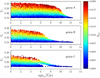 |
Fig. 10. Predicted He mass fraction in the stellar populations of our three reference galaxies as a function of the stellar ages. The colour coding corresponds to the O mass fraction of the stars. Each panel, from top to bottom, shows our predictions for each reference galaxy, from galaxy A to galaxy C, respectively. |
Our findings in Fig. 10 can be easily interpreted in light of our previous results in Sect. 4.1. In particular, at any given galactocentric radius on the galaxy disc, stellar populations of different ages and metallicities cohabit, depending on how the past star formation activity was distributed in space as a function of time. Therefore, for a given age of the stars, there is a distribution of metallicities, which automatically translate into Y variations. At any given bin of stellar age, the star particles with the lowest metallicities were typically born in the galaxy outermost regions, where – because of the inside-out growth of the galactic disc – the chemical enrichment timescales are typically long. This gives rise to low He abundances in the galaxy outer regions, close to Y ∼ 0.24, which is approximately the primordial value.
To understand the impact of different stellar ages on the predicted He abundances, we divide the stellar populations in Fig. 10 into different bins of metallicity, with widths of 0.1dex in logarithmic units, and – for each bin – we compute the dispersion of the He abundances, σY⋆, as due to the variation of the stellar ages in the bin. Our results are shown in Fig. 11. We find that the dispersion of the He content due to different stellar ages increases as a function of metallicity, reaching values as high as ≈0.007 for galaxy A, which corresponds to ∼12% of the predicted global variation of Y within the galaxy.
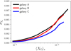 |
Fig. 11. Dispersion of the He abundances in the stellar populations of our simulated disc galaxies, σY⋆, considering different metallicity bins, ⟨XO⟩⋆, with widths of 0.1 dex in logarithmic units, as obtained from the analysis of Fig. 10. |
In Fig. 12, we present a set of one-zone chemical-evolution models (similar to those described in Sect. 3) assuming the same IMF, stellar lifetimes, and stellar nucleosynthetic yields as in our cosmological hydrodynamical simulation. In this set of models, we assume SFE = 2 Gyr−1, no galactic winds, and we vary the infall timescale from τ = 1 to 10 Gyr, with a step of 0.1 Gyr, to determine whether the inside-out growth of the galaxy disc has an impact on the predicted Y vs. age relation. In particular, in the context of the inside-out growth of galaxies, shorter infall time scales correspond to more central galaxy regions. In Fig. 12a, the colour coding represents the infall timescale, whereas in Fig. 12b the colour coding represents the gas-phase metallicity.
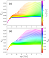 |
Fig. 12. Set of one-zone chemical evolution models assuming the same IMF, stellar lifetimes, and stellar nucleosynthetic yields as in our cosmological hydrodynamical simulation. In the chemical evolution models, we assume SFE = 2 Gyr−1, no galactic winds, and we vary the infall timescale from τ = 1 to 10 Gyr, with a step of 0.1 Gyr, to understand whether the inside-out growth of galaxies has an impact on the predicted He abundances. In panel a, the colour coding represents the infall timescale, whereas in panel b the colour coding represents the gas-phase metallicity. |
Since the assumed SFE in our chemical-evolution models would only systematically shift the Y − Z and Y–age relations along the y-axis, making the chemical enrichment faster or slower as a function of time (if one increases or decreases the SFE, respectively), Fig. 12 demonstrates that the inside-out growth of the galaxy disc is the main effect regulating the evolution of the He abundances in galaxies. In particular, diminishing the infall timescale (namely, moving towards inner galaxy regions) leads to a faster chemical enrichment in the galaxy, giving rise to higher metallicities and He abundances for a fixed age. Our chemical-evolution models therefore predict that the innermost galaxy regions (e.g. bulge and inner disc) have steeper Y vs. age relations at high metallicities than the outermost galaxy regions.
In Fig. 13 we investigate how Y⋆ − XO, ⋆ (left panels) and Y⋆ − XN, ⋆ (right panels) in the stars of our simulated galaxies depend on [α/Fe]⋆ (colour coding, where we assume O as a proxy for the α-elements). There is a trend, according to which the high-[α/Fe] stars have flatter Y⋆ − XO, ⋆ and steeper Y⋆ − XN, ⋆ relations than the low-[α/Fe] stars, even though the predicted spread in Y⋆ − XO, ⋆ is larger than that in Y⋆ − XN, ⋆. These predictions are consistent with our results on the temporal evolution of dY/dXO and dY/dXN in the ISM (see Fig. 6, top and bottom panels).
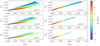 |
Fig. 13. Predicted Y⋆ − XO, ⋆ (left panels) and Y⋆ − XN, ⋆ (right panels) in the stellar populations of our three reference galaxies (from top to bottom). The colour coding represents the [α/Fe]⋆ ratios of the stars. |
Finally, since in Fig. 13 we show our predictions for the [O/Fe]⋆ ratios, we show that our simulation can produce reasonable results also for the classical [O/Fe]⋆ − [Fe/H]⋆ diagram in Fig. 14, where the colour-coding corresponds to the He content of the stars, Y⋆. Nevertheless, we caution the readers that Fe and O are produced by Type Ia and core-collapse SNe, respectively, on very different typical timescales from the star formation event.
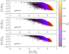 |
Fig. 14. Predicted [O/Fe]⋆ − [Fe/H]⋆ diagrams in the stellar populations of our three reference simulated galaxies, with the colour coding representing the He content, Y⋆, of the stars. |
4.4. Comparison with the observed He abundances in the stars
In Fig. 15, we compare the predictions of our simulation for Y⋆ vs. [Fe/H]⋆ in galaxies A–C with the observations. In particular, we show the observed He abundances in the Galactic open cluster NGC 6791 (McKeever et al. 2019), in a sample of horizontal branch stars in M 30 and NGC 6397 (Mucciarelli et al. 2014), as well as in a sample of RR Lyrae in the Galactic bulge (Marconi & Minniti 2018). We also show the He abundances in a sample of B-type stars within the solar neighbourhood from Nieva & Przybilla (2012), and the initial He abundance of the Sun from Serenelli & Basu (2010). Even though some of the observed data in Fig. 15 represent indirect measurements of He in stars (apart from the stellar data of Nieva & Przybilla 2012; Mucciarelli et al. 2014), and we did not choose our simulated galaxies to reproduce the observed He abundances in the MW, the predicted trend of Y⋆ vs. [Fe/H]⋆ qualitatively agrees with the observed trend, despite the fact that our model predictions always lie below the observed MW data at high metallicities.
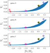 |
Fig. 15. Comparison of our predicted Y⋆ vs. [Fe/H]⋆ relations in galaxies A–C (from top to bottom; light blue points) with the observed data of Mucciarelli et al. (2014, red squared) for blue horizontal-branch stars in the Galactic globular clusters M 30 and NGC 6397, Marconi & Minniti (2018, magenta pentagon) for a sample of RR Lyrae in the Galactic bulge, the He abundances in the Galactic open cluster NGC 6791 from McKeever et al. (2019, blue circle), and the He abundances in a sample of B-type stars within the solar neighbourhood from Nieva & Przybilla (2012, black star). The yellow star corresponds to the initial He abundance of the Sun (Serenelli & Basu 2010), for which [Fe/H] is computed assuming that the iron mass fraction scales with total metallicity, as in the solar photospheric chemical composition as derived by Grevesse & Sauval (1998). |
Finally, in Fig. 16, we compare the predictions of our simulation for (He/H)⋆ vs. [Fe/H]⋆ in galaxies A–C with the observed He abundances in Galactic B-type stars, as measured by Morel et al. (2006). For reference we also show the value of the typical He abundance of B-type stars (Nieva & Przybilla 2012) and the initial He abundance of the Sun from Serenelli & Basu (2010). The observed data in Fig. 16 represent direct He abundance measurements in the stars, and we predict a much less scattered relation than in the observed data, even though our predicted values for (He/H)⋆ are qualitatively consistent with observations.
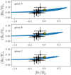 |
Fig. 16. Comparison of our predicted (He/H)⋆ vs. [Fe/H]⋆ relations in galaxies A–C (from top to bottom; light blue points) with the observed data of Morel et al. (2006, black points with error bars) for B-type stars. We also show the value of the typical He abundance in a sample of B-type stars within the solar neighbourhood from Nieva & Przybilla (2012, black star). The yellow star corresponds to the initial He abundance in the Sun (Serenelli & Basu 2010), where we scale the Fe abundances with respect to the solar photospheric abundance of Fe from Grevesse & Sauval (1998). |
Galactic globular clusters are nowadays known to host multiple stellar populations, which clearly show up both in their observed CMD (particularly when combining passbands with different response to the molecule bands of OH, CN, CH, and NH; see, e.g. Milone et al. 2012) and in their light-element chemical abundance patterns (see, e.g. Gratton et al. 2004, 2012; Prantzos & Charbonnel 2006; Milone et al. 2013). The He content in the different stellar populations of globular clusters can be inferred by means of a precise isochrone-fitting analysis; in particular, stars with higher Y are more luminous and tend to have bluer colours, especially at high metallicities (Milone et al. 2018). One of the most puzzling results in globular cluster studies is that their latest generations of stars have enhanced He abundances, which can be as high as Y ≈ 0.4 (e.g. D’Antona et al. 2002, 2005; Piotto et al. 2005, 2007); this has also been confirmed with direct spectroscopic He abundance measurements in globular cluster horizontal branch stars (Marino 2014). Finally, such He-enhancement has been found to strongly correlate with the cluster mass, being larger in more massive clusters (e.g. Milone 2015).
In our cosmological hydrodynamical simulation, the typical mass of the star particles at redshift z = 0 is in the range ≈105−106 M⊙, hence of the order of globular cluster mass. Our simulation cannot naturally predict any He spread within the star particles, because – by construction – the latter are simple stellar populations, with fixed age and metallicity. Moreover, the appearance of multiple stellar populations in globular clusters would be a sub-resolution process in our simulation, which could only be included through some parametrisation, without emerging from the simulation itself, like for example our predicted He enhancement in the central, denser galaxy regions, which is a natural outcome of the cosmological inside-out growth of the galaxy disc as a function of time. Therefore, in conclusion, if we suppose that our star particles represent globular clusters, and therefore our simulation can provide only an average He content between all the underlying stellar populations.
5. Conclusions
In this paper, we show for the first time how He abundance in star-forming disc galaxies evolves as a function of time, chemical composition, and SFH in the context of cosmological chemodynamical simulations (Kobayashi et al. 2007; Vincenzo & Kobayashi 2018a,b). We believe that the results of our study will be of great interest for a wide range of subdisciplines in stellar physics, in which the assumed calibration between Y and Z represents one of the major sources of systematic uncertainty, being largely unknown.
Our main conclusions can be summarised as follows.
-
1.
The predicted Y − XC,N,O relations in galaxies depend on their past SFH (see Figs. 5 and 6). In particular, young galaxies have – on average – flatter Y − XC,O and steeper Y − XN relations than the old ones.
-
2.
We find that dY/dZ depends on the galaxy SFH and is not constant as a function of time. Moreover, the temporal evolution of dY/dZ depends on the particular chemical element used to trace Z
-
3.
The predicted temporal evolution of dY/dXO in the ISM is opposite with respect to that of dY/dXN (see Fig. 6). In particular dY/dXO increases – on average – as a function of time, whereas dY/dXN decreases, because N is mostly synthesised as a secondary element, with its stellar yields strongly increasing as a function of metallicity. Finally, we find that dY/dXC weakly increases as a function of time, because He and C are strictly coupled from a nucleosynthesis point of view. Interestingly, Y − XC+N depends very weakly on the galaxy SFH, having values in the range ≈[6.4, 6.6].
-
4.
The predicted Y − XC and Y − XN relations are steeper and less scattered than Y − XO (see Figs. 5 and 6). This suggests that C, N, or C+N abundances are more appropriate as metallicity calibrators for stellar models than that of O.
-
5.
Our predicted values for dY/dXO are in relatively good agreement with the observed relations in extragalactic HII regions (Izotov et al. 2007); however, our predicted values for dY/dZ are lower than those found with indirect He abundance measurements in large samples of stars in our Galaxy (Jimenez et al. 2003; Casagrande et al. 2007; Portinari et al. 2010), as well in Galactic open clusters (Brogaard et al. 2012). This is likely due to the large uncertainty in the He nucleosynthesis from AGB stars in our cosmological simulation. For example, by assuming the Ventura et al. (2013) stellar yields for AGB stars, we obtain a steeper Y − Z relation than that found with the Karakas (2010) stellar yields, with a difference in dY/dZ which can be as large as ≈0.35. Nevertheless, the observed dY/dZ values in the stars still suffer from some uncertainty, because of the typical indirect methods employed to measure He abundances, which depend on the assumptions of stellar models (e.g. Casagrande et al. 2007; Portinari et al. 2010).
-
6.
We predict radial gradients of Y in the ISM of our simulated disc galaxies, according to which the central regions have – on average – higher Y and metallicities than the outermost regions (see Fig. 5). This is due to an inside-out growth of the stellar mass (and to an inside-out propagation of the star formation activity) in our simulated disc galaxies as a function of time (see also Vincenzo & Kobayashi 2018b), the main effect of which – from the point of view of chemical evolution – is an increase of the typical chemical enrichment timescale as a function of the galactocentric distance, giving rise to higher average Y and Z values in the centre.
-
7.
We find that, at fixed O/H, the predicted gas-phase He/H abundances increase as a function of time, with this increase being faster in the inner galaxy regions (see Fig. 7). We conclude that this is an effect of the inside-out growth of our simulated disc galaxies as a function of time.
-
8.
By comparing our simulations with the observed He/H abundances in a sample of low-metallicity star-forming galaxies from Aver et al. (2015) and Fernández et al. (2019), we predict much more homogeneous gas-phase He/H abundances at low metallicities than in the observed data set (see Fig. 7). This may be due to the fact that the galaxies of the observed sample are relatively metal-poor with ongoing star formation activity at the present time, whereas the low-metallicity environments in our simulated disc galaxies at the present time correspond to the galaxy outer regions, where there is no sign of recent strong star formation activity. Nevertheless, we also discuss that this disagreement in the scatter may be due to the limited resolution of our simulation, as well as to chemical enrichment from rotating massive Wolf–Rayet stars (Kumari et al. 2018), which are not included in our cosmological simulation.
-
9.
For a fixed stellar metallicity bin, the variation of Y⋆ due to different stellar ages becomes increasingly important with increasing metallicity (see Fig. 11). Since the stars in the bulge and in the inner disc of galaxies typically have the highest metallicities, we expect that the impact of stellar age on the variation of He abundance becomes more important in the inner galaxy regions; in particular, we find that for the typical high metallicities of Galactic bulge stars, the variation of Y⋆ contributed by different stellar ages can be as high as ∼12% with respect to the global variation of Y⋆. On the other hand, in the galaxy disc, the metallicity is the most important quantity determining the variation of Y⋆ in the galaxy. Nevertheless, the systematic uncertainty introduced by different stellar yield assumptions for AGB stars is comparable to the spread that we find for Y⋆ at high metallicity, which is of the order of ≈0.007.
-
10.
By making use of chemical evolution models with different infall timescales, we find that the innermost galactic regions (which are characterised by shorter infall timescales according to the inside-out scenario) have steeper Y vs. age relations at high metallicities than the outermost disc regions (see Fig. 12).
-
11.
The predicted Y⋆ − XO, ⋆ relation in the stars is very sensitive to [α/Fe]. In particular, the high-[α/Fe] stars exhibit a flatter average relation than those with low [α/Fe]. An opposite but weaker trend is found for Y⋆ − XN, ⋆ when considering stars with different [α/Fe] (see Fig. 13).
-
12.
Even though we did not choose our simulated disc galaxies to reproduce the observed chemical abundances of He in our Galaxy, the predicted trend of our simulations for Y⋆ vs. [Fe/H]⋆ qualitatively agrees with observations.
We address the readers to the following website hosted by the University of Rochester for a referenced list of measured dY/dZ from different sources in the literature, put together by Eric Mamajek: http://www.pas.rochester.edu/~emamajek/memo_dydz.html
These galaxies ABC are different from the sample in Vincenzo & Kobayashi (2018a).
Acknowledgments
We thank an anonymous referee for many constructive comments, which greatly improved the quality and clarity of our paper. Moreover, we thank Emma Willett for many useful discussions. FV, AM, JTM, and JM acknowledge support from the European Research Council Consolidator Grant funding scheme (project ASTEROCHRONOMETRY, G.A. n. 772293). CK acknowledges funding from the United Kingdom Science and Technology Facility Council (STFC) through grant ST/R000905/1. This work used the DiRAC Data Centric system at Durham University, operated by the Institute for Computational Cosmology on behalf of the STFC DiRAC HPC Facility (www.dirac.ac.uk). This equipment was funded by a BIS National E-infrastructure capital grant ST/K00042X/1, STFC capital grant ST/K00087X/1, DiRAC Operations grant ST/K003267/1 and Durham University. DiRAC is part of the National E-Infrastructure. This research has made use of University of Hertfordshire’s high-performance computing facility. We finally thank Volker Springel for providing GADGET-3.
References
- Aver, E., Olive, K. A., & Skillman, E. D. 2015, JCAP, 2015, 011 [Google Scholar]
- Balser, D. S. 2006, AJ, 132, 2326 [NASA ADS] [CrossRef] [Google Scholar]
- Beasor, E. R., & Davies, B. 2018, MNRAS, 475, 55 [NASA ADS] [CrossRef] [Google Scholar]
- Bensby, T., Feltzing, S., & Oey, M. S. 2014, A&A, 562, A71 [NASA ADS] [CrossRef] [EDP Sciences] [Google Scholar]
- Brogaard, K., VandenBerg, D. A., Bruntt, H., et al. 2012, A&A, 543, A106 [NASA ADS] [CrossRef] [EDP Sciences] [Google Scholar]
- Casagrande, L., Flynn, C., Portinari, L., Girardi, L., & Jimenez, R. 2007, MNRAS, 382, 1516 [NASA ADS] [CrossRef] [Google Scholar]
- Casagrande, L., Silva Aguirre, V., Schlesinger, K. J., et al. 2016, MNRAS, 455, 987 [NASA ADS] [CrossRef] [Google Scholar]
- Chabrier, G. 2003, PASP, 115, 763 [NASA ADS] [CrossRef] [Google Scholar]
- Chiappini, C., Renda, A., & Matteucci, F. 2002, A&A, 395, 789 [NASA ADS] [CrossRef] [EDP Sciences] [Google Scholar]
- Chiosi, C., & Matteucci, F. M. 1982, A&A, 105, 140 [NASA ADS] [Google Scholar]
- Cooke, R. J., & Fumagalli, M. 2018, Nat. Astron., 2, 957 [NASA ADS] [CrossRef] [Google Scholar]
- D’Antona, F., Caloi, V., Montalbán, J., Ventura, P., & Gratton, R. 2002, A&A, 395, 69 [NASA ADS] [CrossRef] [EDP Sciences] [Google Scholar]
- D’Antona, F., Bellazzini, M., Caloi, V., Pecci, F. F., Galleti, S., & Rood, R. T. 2005, ApJ, 631, 868 [NASA ADS] [CrossRef] [Google Scholar]
- Fernández, V., Terlevich, E., Díaz, A. I., Terlevich, R., & Rosales-Ortega, F. F. 2018, MNRAS, 478, 5301 [NASA ADS] [CrossRef] [Google Scholar]
- Fernández, V., Terlevich, E., Díaz, A. I., et al. 2019, MNRAS, 487, 3221 [NASA ADS] [CrossRef] [Google Scholar]
- Fields, B. D. 1996, ApJ, 456, 478 [NASA ADS] [CrossRef] [Google Scholar]
- Gennaro, M., Prada Moroni, P. G., & Degl’Innocenti, S. 2010, A&A, 518, A13 [NASA ADS] [CrossRef] [EDP Sciences] [Google Scholar]
- Gratton, R., Sneden, C., & Carretta, E. 2004, ARA&A, 42, 385 [NASA ADS] [CrossRef] [Google Scholar]
- Gratton, R. G., Carretta, E., & Bragaglia, A. 2012, A&ARv, 20, 50 [CrossRef] [Google Scholar]
- Grevesse, N., & Sauval, A. J. 1998, Sci Space Rev., 85, 161 [CrossRef] [Google Scholar]
- Hinshaw, G., Larson, D., Komatsu, E., et al. 2013, ApJS, 208, 19 [NASA ADS] [CrossRef] [Google Scholar]
- Iben, I. 1968, Nature, 220, 143 [NASA ADS] [CrossRef] [Google Scholar]
- Iben, I., & Renzini, A. 1983, ARA&A, 21, 271 [NASA ADS] [CrossRef] [Google Scholar]
- Izotov, Y. I., Thuan, T. X., & Stasińska, G. 2007, ApJ, 662, 15 [NASA ADS] [CrossRef] [Google Scholar]
- Izotov, Y. I., Thuan, T. X., & Guseva, N. G. 2014, MNRAS, 445, 778 [NASA ADS] [CrossRef] [Google Scholar]
- Jimenez, R., Flynn, C., MacDonald, J., & Gibson, B. K. 2003, Science, 299, 1552 [NASA ADS] [CrossRef] [PubMed] [Google Scholar]
- Karakas, A. I. 2010, MNRAS, 403, 1413 [NASA ADS] [CrossRef] [Google Scholar]
- Karakas, A. I., & Lattanzio, J. C. 2007, PASA, 24, 103 [NASA ADS] [CrossRef] [Google Scholar]
- Karakas, A. I., & Lugaro, M. 2016, ApJ, 825, 26 [NASA ADS] [CrossRef] [Google Scholar]
- Karakas, A. I., Lattanzio, J. C., & Pols, O. R. 2002, PASA, 19, 515 [NASA ADS] [CrossRef] [Google Scholar]
- Karakas, A. I., Lugaro, M., Carlos, M., et al. 2018, MNRAS, 477, 421 [NASA ADS] [CrossRef] [Google Scholar]
- Kobayashi, C. 2004, MNRAS, 347, 740 [NASA ADS] [CrossRef] [Google Scholar]
- Kobayashi, C., Springel, V., & White, S. D. M. 2007, MNRAS, 376, 1465 [Google Scholar]
- Kobayashi, C., Karakas, A. I., & Umeda, H. 2011, MNRAS, 414, 3231 [NASA ADS] [CrossRef] [Google Scholar]
- Kroupa, P. 2008, in Pathways Through an Eclectic Universe, ASP Conf. Ser., 390, 3 [NASA ADS] [Google Scholar]
- Kumari, N., James, B. L., Irwin, M. J., Amorín, R., & Pérez-Montero, E. 2018, MNRAS, 476, 3793 [NASA ADS] [CrossRef] [Google Scholar]
- Lebreton, Y., Goupil, M. J., & Montalbán, J. 2014, EAS Publ. Ser., 65, 99 [CrossRef] [EDP Sciences] [Google Scholar]
- Limongi, M., & Chieffi, A. 2018, ApJS, 237, 13 [NASA ADS] [CrossRef] [Google Scholar]
- Luridiana, V., Peimbert, A., Peimbert, M., & Cerviño, M. 2003, ApJ, 592, 846 [NASA ADS] [CrossRef] [Google Scholar]
- Maeder, A. 2009, Astronomy and Astrophysics Library (Berlin, Heidelberg: Springer) [CrossRef] [Google Scholar]
- Marconi, M., & Minniti, D. 2018, ApJ, 853, L20 [NASA ADS] [CrossRef] [Google Scholar]
- Marino, A. F., Milone, A. P., Przybilla, N., et al. 2014, MNRAS, 437, 1609 [NASA ADS] [CrossRef] [Google Scholar]
- Miglio, A., Chiappini, C., Mosser, B., et al. 2017, Astron. Nachr., 338, 644 [NASA ADS] [CrossRef] [Google Scholar]
- Milone, A. P. 2015, MNRAS, 446, 1672 [NASA ADS] [CrossRef] [Google Scholar]
- Milone, A. P., Piotto, L. R., Bedin, I. R., et al. 2012, ApJ, 744, 58 [NASA ADS] [CrossRef] [Google Scholar]
- Milone, A. P., Marino, A. F., Piotto, G., et al. 2013, ApJ, 767, 120 [NASA ADS] [CrossRef] [Google Scholar]
- Milone, A. P., Marino, A. F., Renzini, A., et al. 2018, MNRAS, 481, 5098 [NASA ADS] [CrossRef] [Google Scholar]
- Morel, T., Butler, K., Aerts, C., Neiner, C., & Briquet, M. 2006, A&A, 457, 651 [NASA ADS] [CrossRef] [EDP Sciences] [Google Scholar]
- Mucciarelli, A., Lovisi, L., Lanzoni, B., & Ferraro, F. R. 2014, ApJ, 786, 14 [NASA ADS] [CrossRef] [Google Scholar]
- Müller, B., Heger, A., Liptai, D., & Cameron, J. B. 2016, MNRAS, 460, 742 [NASA ADS] [CrossRef] [Google Scholar]
- McKeever, J. M., Basu, S., & Corsaro, E. 2019, ApJ, 874, 180 [NASA ADS] [CrossRef] [Google Scholar]
- Nataf, D. M., & Gould, A. P. 2012, ApJ, 751, L39 [NASA ADS] [CrossRef] [Google Scholar]
- Nieva, M.-F., & Przybilla, N. 2012, A&A, 539, A143 [NASA ADS] [CrossRef] [EDP Sciences] [Google Scholar]
- Nomoto, K., Kobayashi, C., & Tominaga, N. 2013, ARA&A, 51, 457 [NASA ADS] [CrossRef] [Google Scholar]
- Olive, K. A., & Skillman, E. D. 2004, ApJ, 617, 29 [NASA ADS] [CrossRef] [Google Scholar]
- Pagel, B. E. J., & Portinari, L. 1998, MNRAS, 298, 747 [NASA ADS] [CrossRef] [Google Scholar]
- Peimbert, M., & Torres-Peimbert, S. 1976, ApJ, 203, 581 [NASA ADS] [CrossRef] [Google Scholar]
- Peimbert, A., Peimbert, M., & Luridiana, V. 2002, ApJ, 565, 668 [NASA ADS] [CrossRef] [Google Scholar]
- Peimbert, M., Peimbert, A., & Delgado-Inglada, G. 2017, PASP, 129, 082001 [NASA ADS] [CrossRef] [Google Scholar]
- Piotto, G., Villanova, S., Bedin, L. R., et al. 2005, ApJ, 621, 777 [NASA ADS] [CrossRef] [Google Scholar]
- Piotto, G., Bedin, L. R., Anderson, J., et al. 2007, ApJ, 661, L53 [NASA ADS] [CrossRef] [Google Scholar]
- Portinari, L., Casagrande, L., & Flynn, C. 2010, MNRAS, 406, 1570 [NASA ADS] [Google Scholar]
- Pottasch, S. R., & Bernard-Salas, J. 2010, A&A, 517, A95 [NASA ADS] [CrossRef] [EDP Sciences] [Google Scholar]
- Prantzos, N., & Charbonnel, C. 2006, A&A, 458, 135 [NASA ADS] [CrossRef] [EDP Sciences] [Google Scholar]
- Prantzos, N., Abia, C., Limongi, M., Chieffi, A., & Cristallo, S. 2018, MNRAS, 476, 3432 [NASA ADS] [CrossRef] [Google Scholar]
- Renzini, A. 2015, ASP Conf. Ser., 497, 1 [Google Scholar]
- Renzini, A., Gennaro, M., Zoccali, M., et al. 2018, ApJ, 863, 16 [NASA ADS] [CrossRef] [Google Scholar]
- Romano, D., Matteucci, F., Tosi, M., et al. 2007, MNRAS, 376, 405 [NASA ADS] [CrossRef] [Google Scholar]
- Serenelli, A. M., & Basu, S. 2010, ApJ, 719, 865 [NASA ADS] [CrossRef] [Google Scholar]
- Shetrone, M., Tayar, J., Johnson, J. A., et al. 2019, ApJ, 872, 137 [NASA ADS] [CrossRef] [Google Scholar]
- Shipman, H. L., & Strom, S. E. 1970, ApJ, 159, 183 [NASA ADS] [CrossRef] [Google Scholar]
- Silva Aguirre, V., & Serenelli, A. M. 2016, Astron. Nachr., 337, 823 [NASA ADS] [CrossRef] [Google Scholar]
- Silva Aguirre, V., Bojsen-Hansen, M., Slumstrup, D., et al. 2018, MNRAS, 475, 5487 [NASA ADS] [Google Scholar]
- Smartt, S. J. 2009, ARA&A, 47, 63 [NASA ADS] [CrossRef] [Google Scholar]
- Springel, V. 2005, MNRAS, 364, 1105 [NASA ADS] [CrossRef] [Google Scholar]
- Stanghellini, L., Guerrero, M. A., Cunha, K., Manchado, A., & Villaver, E. 2006, ApJ, 651, 898 [NASA ADS] [CrossRef] [Google Scholar]
- Struve, O. 1928, Nature, 122, 994 [NASA ADS] [CrossRef] [Google Scholar]
- Sukhbold, T., & Adams, S. 2019, MNRAS, submitted [arXiv:1905.00474] [Google Scholar]
- Valerdi, M., Peimbert, A., Peimbert, M., & Sixtos, A. 2019, ApJ, 876, 98 [NASA ADS] [CrossRef] [Google Scholar]
- Vangioni, E., Dvorkin, I., Olive, K. A., et al. 2018, MNRAS, 477, 56 [NASA ADS] [CrossRef] [Google Scholar]
- Ventura, P., Di Criscienzo, M., Carini, R., & D’Antona, F. 2013, MNRAS, 431, 3642 [NASA ADS] [CrossRef] [Google Scholar]
- Vincenzo, F., & Kobayashi, C. 2018a, A&A, 610, L16 [NASA ADS] [CrossRef] [EDP Sciences] [Google Scholar]
- Vincenzo, F., & Kobayashi, C. 2018b, MNRAS, 478, 155 [NASA ADS] [CrossRef] [Google Scholar]
- Vincenzo, F., Belfiore, F., Maiolino, R., Matteucci, F., & Ventura, P. 2016, MNRAS, 458, 3466 [NASA ADS] [CrossRef] [Google Scholar]
All Figures
|
Fig. 1. Predicted age distribution of the stellar populations in our three reference galaxies. The curves are such that the area below each of them corresponds to the galaxy stellar mass at redshift z = 0. |
| In the text | |
|
Fig. 2. (a) Average IMF-weighted stellar yield of He from massive stars as a function of the initial stellar metallicity, as predicted by the stellar models of Nomoto et al. (2013, black solid line) and Limongi & Chieffi (2018) for different stellar rotational velocities; in particular, the blue, green, and orange lines correspond to the Limongi & Chieffi (2018) stellar models with vrot = 0, 150, and 300 km s−1, respectively. (b) Average IMF-weighted stellar yield of He from AGB stars as a function of initial stellar metallicity, as predicted by the stellar models of Karakas (2010, black solid line) and Ventura et al. (2013, blue solid line). |
| In the text | |
|
Fig. 3. Predicted ejection rate of He from stellar populations of different metallicities (different colours) by assuming the stellar yields of Nomoto et al. (2013). The grey shaded area corresponds to our predictions when assuming the Limongi & Chieffi (2018) set of stellar yields of rotating massive stars with different metallicities ([Fe/H] = 0, −1, −2, and −3 dex) and stellar rotational velocities (vrot = 0, 150, and 300 km s−1). The blue shaded horizontal region corresponds to the chemical enrichment of super-AGB stars which are not included in our galactic chemical evolution model. |
| In the text | |
|
Fig. 4. Effect of different nucleosynthesis yields for massive stars (panels a and c) and AGB stars (panels b and d) on the predicted Y vs. Z relation from a one-zone galaxy chemical evolution model with star formation efficiency SFE = 2 Gyr−1, infall timescale τ = 4 Gyr, and no galactic winds. For massive stars we explore the stellar yields of Nomoto et al. (2013), which are adopted in our cosmological simulations, and the stellar yields of Limongi & Chieffi (2018) for different stellar rotational velocities (v0, v150 and v300 represent rotational velocity v = 0, 150, and 300 km s−1, respectively). For AGB stars, we explore the stellar yields of Karakas (2010), adopted in our cosmological simulations, and those of Ventura et al. (2013); see also e.g. Vincenzo et al. (2016). |
| In the text | |
|
Fig. 5. First row (top): gas-phase He mass fraction, Ygas, as a function of the gas-phase O mass fraction, XO,gas. Second row: Ygas vs. XC,gas. Third row: Ygas vs. XN,gas. Fourth row: Ygas vs. XC+N,gas. Fifth row (bottom): predictions for the radial profile of Ygas as a function of the galactocentric distance, d, with the colour coding representing the O mass fraction. From left to right, the various columns correspond to each of our reference galaxies, from galaxy A to galaxy C, respectively. |
| In the text | |
|
Fig. 6. Predicted evolution of dYgas/dXO (top panel), dYgas/dXC (second panel), dYgas/dXN (third panel), dYgas/dXC+N (third panel), and dYgas/dZ (bottom panel) as a function of look-back time. The black, red, and blue curves correspond to galaxies A, B, and C, respectively. The values of dYgas/dXC,N,O,Z correspond to our best-fit values for the predicted Ygas − XC,N,O,Z relations in each galaxy, by assuming a simple linear law at all times. We only show the evolution of the slopes for times when the galaxy stellar mass M⋆ > 5 × 10⁹ M⊙. |
| In the text | |
|
Fig. 7. Redshift evolution of the gas-phase He/H−O/H abundance pattern in our three simulated disc galaxies. The blue points correspond to the predicted gas-phase abundances at redshift z = 0, orange points to z = 0.5, green points to z = 1, and red points to z = 2. The black and grey triangles with error bars correspond to the observational data of Aver et al. (2015) for a sample of metal-poor HII regions within 16 emission-line galaxies in the Local Universe; the black triangles correspond to their qualifying sample, whereas the grey triangles mark the abundances affected by large systematic uncertainty. Finally, the magenta points with error bars correspond to the observational data of Fernández et al. (2019). |
| In the text | |
|
Fig. 8. Evolution of the average SFR-weighted He/H abundance as a function of the gas fraction (fgas = Mgas/(Mgas + M⋆)) within our simulated disc galaxies. Blue points correspond to galaxy A, orange points to galaxy B, and green points to galaxy C. |
| In the text | |
|
Fig. 9. Predicted gas-phase He/H−O/H abundance pattern at redshift z = 0 in our three simulated disc galaxies, by assuming failed SNe (blue points), like in our reference cosmological hydrodynamical simulation, and by running a similar simulation without failed SNe (orange points). |
| In the text | |
|
Fig. 10. Predicted He mass fraction in the stellar populations of our three reference galaxies as a function of the stellar ages. The colour coding corresponds to the O mass fraction of the stars. Each panel, from top to bottom, shows our predictions for each reference galaxy, from galaxy A to galaxy C, respectively. |
| In the text | |
|
Fig. 11. Dispersion of the He abundances in the stellar populations of our simulated disc galaxies, σY⋆, considering different metallicity bins, ⟨XO⟩⋆, with widths of 0.1 dex in logarithmic units, as obtained from the analysis of Fig. 10. |
| In the text | |
|
Fig. 12. Set of one-zone chemical evolution models assuming the same IMF, stellar lifetimes, and stellar nucleosynthetic yields as in our cosmological hydrodynamical simulation. In the chemical evolution models, we assume SFE = 2 Gyr−1, no galactic winds, and we vary the infall timescale from τ = 1 to 10 Gyr, with a step of 0.1 Gyr, to understand whether the inside-out growth of galaxies has an impact on the predicted He abundances. In panel a, the colour coding represents the infall timescale, whereas in panel b the colour coding represents the gas-phase metallicity. |
| In the text | |
|
Fig. 13. Predicted Y⋆ − XO, ⋆ (left panels) and Y⋆ − XN, ⋆ (right panels) in the stellar populations of our three reference galaxies (from top to bottom). The colour coding represents the [α/Fe]⋆ ratios of the stars. |
| In the text | |
|
Fig. 14. Predicted [O/Fe]⋆ − [Fe/H]⋆ diagrams in the stellar populations of our three reference simulated galaxies, with the colour coding representing the He content, Y⋆, of the stars. |
| In the text | |
|
Fig. 15. Comparison of our predicted Y⋆ vs. [Fe/H]⋆ relations in galaxies A–C (from top to bottom; light blue points) with the observed data of Mucciarelli et al. (2014, red squared) for blue horizontal-branch stars in the Galactic globular clusters M 30 and NGC 6397, Marconi & Minniti (2018, magenta pentagon) for a sample of RR Lyrae in the Galactic bulge, the He abundances in the Galactic open cluster NGC 6791 from McKeever et al. (2019, blue circle), and the He abundances in a sample of B-type stars within the solar neighbourhood from Nieva & Przybilla (2012, black star). The yellow star corresponds to the initial He abundance of the Sun (Serenelli & Basu 2010), for which [Fe/H] is computed assuming that the iron mass fraction scales with total metallicity, as in the solar photospheric chemical composition as derived by Grevesse & Sauval (1998). |
| In the text | |
|
Fig. 16. Comparison of our predicted (He/H)⋆ vs. [Fe/H]⋆ relations in galaxies A–C (from top to bottom; light blue points) with the observed data of Morel et al. (2006, black points with error bars) for B-type stars. We also show the value of the typical He abundance in a sample of B-type stars within the solar neighbourhood from Nieva & Przybilla (2012, black star). The yellow star corresponds to the initial He abundance in the Sun (Serenelli & Basu 2010), where we scale the Fe abundances with respect to the solar photospheric abundance of Fe from Grevesse & Sauval (1998). |
| In the text | |
Current usage metrics show cumulative count of Article Views (full-text article views including HTML views, PDF and ePub downloads, according to the available data) and Abstracts Views on Vision4Press platform.
Data correspond to usage on the plateform after 2015. The current usage metrics is available 48-96 hours after online publication and is updated daily on week days.
Initial download of the metrics may take a while.