| Issue |
A&A
Volume 630, October 2019
|
|
|---|---|---|
| Article Number | A61 | |
| Number of page(s) | 9 | |
| Section | Astrophysical processes | |
| DOI | https://doi.org/10.1051/0004-6361/201833796 | |
| Published online | 23 September 2019 | |
Optical depth in polarised Monte Carlo radiative transfer
1
Sterrenkundig Observatorium, Universiteit Gent, Krijgslaan 281 S9, 9000 Gent, Belgium
e-mail: This email address is being protected from spambots. You need JavaScript enabled to view it.
2
European Southern Observatory, Karl-Schwarzschild-Straße 2, 85748 Garching bei München, Germany
Received:
9
July
2018
Accepted:
25
July
2019
Abstract
Context. The Monte Carlo method is the most widely used method to solve radiative transfer problems in astronomy, especially in a fully general 3D geometry. A crucial concept in any Monte Carlo radiative transfer code is the random generation of the next interaction location. In polarised Monte Carlo radiative transfer with aligned non-spherical grains, the nature of dichroism complicates the concept of optical depth.
Aims. We investigate, in detail, the relation between optical depth and the optical properties and density of the attenuating medium in polarised Monte Carlo radiative transfer codes that take dichroic extinction into account.
Methods. Based on solutions for the radiative transfer equation, we discuss the optical depth scale in polarised radiative transfer with spheroidal grains. We compare the dichroic optical depth to the extinction and total optical depth scale.
Results. In a dichroic medium, the optical depth is not equal to the usual extinction optical depth, nor to the total optical depth. For representative values of the optical properties of dust grains, the dichroic optical depth can differ from the extinction or total optical depth by several tens of percent. A closed expression for the dichroic optical depth cannot be given, but it can be derived efficiently through an algorithm that is based on the analytical result corresponding to elongated grains with a uniform grain alignment.
Conclusions. Optical depth is more complex in dichroic media than in systems without dichroic attenuation, and this complexity needs to be considered when generating random free path lengths in Monte Carlo radiative transfer simulations. There is no benefit in using approximations instead of the dichroic optical depth.
Key words: radiative transfer / polarization
© ESO 2019
1. Introduction
Radiative transfer is a broad field in astronomy that aims to describe the interaction between radiation and matter. In an astronomical context, the Monte Carlo method is by far the most widely used method to solve radiative transfer problems. In the past decades, many different Monte Carlo codes have been developed to address different astrophysical radiative transfer problems, including photoionisation, absorption and scattering by cosmic dust, the origin of infrared emission, and resonant line scattering heating (e.g. Gordon et al. 2001; Ercolano et al. 2003; Robitaille 2011; Yajima et al. 2012; Whitney et al. 2013; Camps & Baes 2015; Reissl et al. 2016). General reviews on Monte Carlo transport can be found in Dupree & Fraley (2002) or Kalos & Whitlock (2008), for example, and dedicated reviews on radiative transfer in astrophysics include Whitney (2011) and Steinacker et al. (2013).
The essence of the Monte Carlo method is to represent the radiation field as the flow of a large, but finite, number of photon packages. The life cycle of each photon package is followed individually. Additionally, at every stage in this life cycle, the characteristics that determine the path of each photon package are determined in a probabilistic way by generating random numbers from the appropriate probability density function (PDF). At the end of the simulation, the radiation field, or more specifically the intensity of the radiation field, is recovered from a statistical analysis of the photon package paths.
An important ingredient of Monte Carlo radiative transfer is the knowledge of the appropriate PDF for a given characteristic, and the accurate and efficient sampling of random numbers from these PDFs. For some characteristics, the PDFs are simple and sampling random numbers from them is trivial. For example, most sources send out radiation isotropically, which implies that the generation of propagation directions after an emission event simply comes down to generating a random point on the unit sphere. The PDF that controls the random starting positions for the photon package is dictated by the 3D luminosity density of the sources, and specific methods have been developed to generate such random positions from a range of 3D density distributions (Baes & Camps 2015).
An aspect that is central to any Monte Carlo radiative transfer code is the random generation of the next interaction location. More specifically, if a photon package is emitted or scattered into a given direction, one needs to randomly generate a free path length s to the next interaction. To do so, we need to know the appropriate PDF p(s). In this context, the concept of optical depth τ plays a crucial role. In optical depth space, the PDF p(τ) is a simple exponential distribution (Cashwell & Everett 1959; Steinacker et al. 2013). This implies that the next interaction location can be found by randomly generating a random optical depth from an exponential distribution and by converting this optical depth to a physical path length, which is a critical point. We need to know the relation τ(s), or inversely s(τ), to properly calculate the next interaction location.
In radiative transfer problems where polarisation is not taken into account, τ(s) can immediately be calculated from the density and the optical properties along the path. Notably, it does not depend on the intensity of the radiation field. The situation becomes more complex when polarisation comes into play. In the case of spherical or randomly oriented particles, polarised Monte Carlo radiative transfer is only slightly more difficult to use than unpolarised Monte Carlo radiative transfer. The main added complexities are that a Stokes vector needs to be introduced to characterise the polarisation status of each photon package and that this Stokes vector can alter during a scattering event (e.g. Fischer et al. 1994; Code & Whitney 1995; Bianchi et al. 1996; Peest et al. 2017). The relation between optical depth and path length is the same as for unpolarised Monte Carlo radiative transfer.
The real complexity arises when the attenuating particles are non-spherical and aligned, as in the case of elongated dust grains in the interstellar medium. Such dust grains are aligned with respect to the magnetic fields through a variety of processes (Davis & Greenstein 1951; Jones & Spitzer 1967; Aannestad & Greenberg 1983; Lazarian 1994, 2007). An interesting feature is dichroism, which, in this context, means that radiation of different polarisation experience different amounts of extinction. The nature of dichroism complicates the relation between optical depth and physical path length.
In this paper, we investigate in detail whether an optical depth scale can still be used in a meaningful way in polarised Monte Carlo radiative transfer codes that take dichroic extinction into account. In Sect. 2 we discuss optical depth and the generation of random path lengths in standard unpolarised radiative transfer. In Sect. 3 we extend this discussion to polarised radiative transfer in the case of elongated aligned grains, in particular. Apart from the “standard” extinction optical depth, we introduce the total and dichroic optical depth scales, and we compare and analyse them. In Sect. 4 we discuss the implications of these findings for Monte Carlo radiative transfer codes that take dichroic extinction into account. In Sect. 5 we discuss these results and provide a summary.
2. Unpolarised radiative transfer
As discussed in the Introduction, one of the essential steps in the life cycle of a photon package in a Monte Carlo radiative transfer simulation is the calculation of the next interaction location, or equivalently, the physical path length s that is covered before the next interaction. In order to do this, we need to generate a random s from the appropriate probability distribution function p(s). The appropriate PDF p(s) can be determined by considering the variation of the specific intensity I(s) along the path. The probability that the photon package has not interacted along the path between 0 and s is equal to I(s)/I0, while I0 is the specific intensity of the photon package at the start of the path1. Therefore, the density function P(s) can be written as follows:
 (1)
(1)
In general, we define the optical depth τ(s) as
![Mathematical equation: $$ \begin{aligned} \tau (s) = -\ln \left[\frac{I(s)}{I_0}\right]\cdot \end{aligned} $$](/articles/aa/full_html/2019/10/aa33796-18/aa33796-18-eq2.gif) (2)
(2)
By combining these two equations, we find that
 (3)
(3)
and when we take the derivative of this cumulative density function,
 (4)
(4)
This yields the well-know result that the PDF describing the next interaction location is an exponential distribution in optical depth space. Generating a random optical depth can easily be done by picking a uniform deviate 𝒳, setting τ = −ln(1 − 𝒳), and subsequently converting this random τ to a physical path length s.
The difficulty involved is that we need to know the solution I(s) to calculate the optical depth scale. This solution is found by solving the appropriate radiative transfer equation. For a photon package moving through an attenuating medium with density n(s) and extinction cross section Cext(s), the radiative transfer equation reads
 (5)
(5)
It is important to note that no additional emission along the path or scattering into the line-of-sight are included as this is not relevant for this particular photon package. The following equation is a simple first-order ordinary differential equation that is easy to solve:
 (6)
(6)
with the extinction optical depth τext(s) that is defined as
 (7)
(7)
By comparing Eqs. (2) and (6), we see that τ(s) = τext(s). In particular, the optical depth scale, from which random path lengths can be sampled, only depends on the density and optical properties of the material, and not on the properties of the photon package. In this simple case, the only property of the photon package that could matter is I0.
While the strategy described above is conceptually very simple, some challenges need to be addressed. In particular, the conversion of extinction optical depth to physical path length is not usually a straightforward inversion. Except for some simple ideal cases, the conversion needs to be done numerically. In most Monte Carlo radiative transfer codes, the attenuating medium is subdivided into a large number of individual cells, each with a constant density and uniform properties. The codes are typically equipped with a routine to calculate paths through this tessellated medium. The routine returns an ordered list of all the cells m that the path crosses, as well as the length Δsm of the path segments corresponding to the mth cell. Given this ordered list, we can calculate the running values for the path length sm and the optical depth τext, m at the exit point of each cell crossed by the path. The problem is thus reduced to finding the first cell in the array, for which τext, m exceeds the randomly generated value of τext, and subsequently to applying a linear interpolation to convert τext to s2.
These integrations through the dust grid often form the most time-consuming part of a radiative transfer simulation. In order to make these calculations as efficient as possible, especially in 3D geometries, advanced grid construction and grid traversal techniques are required (Niccolini & Alcolea 2006; Bianchi 2008; Lunttila & Juvela 2012; Camps et al. 2013; Saftly et al. 2013, 2014; Hubber et al. 2016).
3. Polarised radiative transfer
3.1. The Stokes formalism
The characterisation of the radiation field by the specific intensity and the corresponding radiative transfer Eq. (5) are no longer suitable when polarisation is considered. In order to take the polarisation state of radiation into account, one can use the Stokes formalism, which characterises the radiation field by means of the 4D Stokes vector
 (8)
(8)
The first Stokes parameter, I, is still the specific intensity. The Stokes parameters Q and U describe the state of linear polarisation and V describes the state of circular polarisation of the radiation. The Stokes parameters are always defined with respect to a reference direction that is to be chosen freely from the plane perpendicular to the propagation direction. For a detailed description of the Stokes vector and its connection to the monochromatic transverse electromagnetic waves, we refer to Mishchenko et al. (2000).
When we consider the full Stokes vector, the simple radiative transfer Eq. (5) becomes
 (9)
(9)
where K is now the extinction matrix, a 4 × 4 matrix that describes how the different Stokes components are affected when radiation passes through the medium.
3.2. Spherical grains
When dust grains are spherical, or non-spherical but arbitrarily oriented, the extinction matrix is a simple diagonal matrix, all components of the Stokes vector are affected in the same way, and
 (10)
(10)
This implies that there is no mixture of the different Stokes components due to extinction, and the solution of the radiative transfer equation can be directly written as
 (11)
(11)
In particular, the specific intensity I(s) still behaves according to Eq. (6), exactly as is the case for non-polarised radiative transfer. Also, in this case, we can immediately conclude that the PDF describing the net interaction location is an exponential distribution in extinction optical depth space.
3.3. Spheroidal grains
Complexity arises when the dust grains are non-spherical and partially aligned. In this case, the extinction matrix K is not a diagonal matrix, but a full 4 × 4 matrix with 16 nonzero cross sections of which only seven are independent (van de Hulst 1957; Hovenier & van der Mee 1996). Fortunately, in the case of spheroidal grains, K is significantly less complex. If we denote the orientation of the grain alignment at a distance s along the path as ψ(s), K can be expressed as (Martin 1974; Wolf et al. 2002)
 (12)
(12)
with ℒ(ψ) as the Mueller rotation matrix,
 (13)
(13)
and Kref as the extinction matrix in the reference frame of the grain,
 (14)
(14)
We note that Kref has only the following three independent elements: the extinction cross section Cext, polarisation cross section Cpol, and circular polarisation cross section Ccpol (Mishchenko et al. 2000; Whitney & Wolff 2002).
The non-diagonal character of the extinction matrix has an important effect on the radiation field; the different components of the Stokes vector are coupled and will get mixed along the path. In particular, radiation that is initially unpolarised can develop linear and even circular polarisation just by propagating through the medium (Serkowski 1962; Martin 1972, 1974).
This dichroism complicates the relation between path length and optical depth. To stress the fact that we deal with dichroic extinction, we use the term dichroic optical depth and use the notation τdic(s) when we consider the optical depth in a dichroic medium. In general we can write that
![Mathematical equation: $$ \begin{aligned} \tau _{\mathrm{dic}}(s) = -\ln \left[\frac{I(s)}{I_0}\right], \end{aligned} $$](/articles/aa/full_html/2019/10/aa33796-18/aa33796-18-eq15.gif) (15)
(15)
where I(s) should now be seen as the first component of the Stokes vector I(s), which is obtained by solving the vector radiative transfer Eq. (9) with K(s), as given by (12).
In the case of spherical grains, we show that τ(s) = τext(s). However, this equivalence does not hold for the general case of spheroidal grains. Indeed, with an extinction matrix given by expression (12), the radiative transfer equation is a set of four coupled first-order ordinary differential equations with varying coefficients. The full solution for I(s), and hence the dichroic optical depth τdic(s), depends on all elements of the extinction matrix and all initial Stokes components. As the extinction optical depth (7) only depends on one single element (K11 = Cext) of the extinction matrix, and as it is independent of the initial polarisation state I0, it is impossible that the dichroic optical depth is equivalent to the extinction optical depth.
One could consider another optical depth scale that does depend on the initial polarisation state of the photon package. An interesting starting point is the total extinction cross section,
 (16)
(16)
introduced by Mishchenko et al. (2000) and Whitney & Wolff (2002). It properly describes the attenuation of an incident beam with the arbitrary initial polarisation state I0. Based on this total extinction cross section, one can define an optical depth scale, which we denote as the total optical depth, in a similar way as for the extinction optical depth (7),
 (17)
(17)
or explicitly,
 (18)
(18)
Despite the increased complexity, it is computationally not much more difficult to employ than the extinction optical depth. Indeed, for a photon package in a Monte Carlo simulation with a given position, propagation direction, and polarisation state, it is relatively easy to compute the total optical depth τtot, m at the entry point of each cell crossed by the path.
We can, however, use analogous reasoning as above to argue that the total optical depth cannot be equivalent to the dichroic optical depth. Indeed, with an extinction matrix given by expression (12), the radiative transfer equation is a set of four coupled first-order ordinary differential equations with varying coefficients. The full solution for I(s), and hence the dichroic optical depth τdic(s), depends on all elements of the extinction matrix and all initial Stokes components. The expression (18) does indeed depend on the initial linear polarisation state of the incoming radiation and the polarisation cross section, but it does not involve any dependency on the circular polarisation cross section Ccpol or the initial circular polarisation V0. As a result, it is impossible that the total extinction is fully equivalent to the dichroic optical depth.
If neither the extinction optical depth nor the total optical depth are equivalent to the dichroic optical depth, one inevitably questions what the correct expression for the dichroic optical depth is. For a medium with non-uniform grain alignment, the following answer is somewhat disappointing: given the non-trivial coupling of all four components of the radiative transfer equation, it is not possible to write down a closed formula for I(s) nor the dichroic optical depth τdic(s). Obtaining the solution I(s) can be achieved numerically using standard vector ordinary differential equation (ODE) solution techniques. One might wonder whether τext or τtot, for which we have a closed expression, are reasonable approximations for the dichroic optical depth. To answer this question, we performed numerical tests.
We adopted a hypothetical example where n(s) = ψ(s) = s, that is, the density of material increases linearly with increasing distance, and the grain alignment rotates around the path. Furthermore, we assumed that the optical properties do not vary along the path, and we set Cext = 1 and Cpol = Ccpol = 0.1 (representative values of the Cpol/Cext ratio go up to 0.3 and more). On the one hand, we calculated the dichroic optical depth τ(s) by numerically solving the vector radiative transfer equation using an explicit Runge–Kutta method with variable step size control. On the other hand, we used Eqs. (7) and (17) to calculate τext(s) and τtot(s), and we calculated the relative differences
 (19)
(19)
We calculated these quantities for initial Stokes vectors, that are 100% linearly polarised, with the linear polarisation angle
 (20)
(20)
by gradually changing between 0° and 90° in steps of 5°.
In the upper left panel of Fig. 1 we show δext as a function of the dichroic optical depth τdic along the path. The extinction optical depth scale has the advantage that it is simple and does not explicitly depend on the polarisation state of the photon package, such that the relation between s and τext can in principle be precomputed. It is clear, however, that τext is a poor approximation for the dichroic optical depth. Depending on the value of Q0/I0, it can either underestimate or overestimate τdic by up to 20 percent. More importantly, the differences between τdic and τext can be large even at small optical depths.
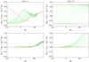 |
Fig. 1. Top left: relative differences δext between extinction optical depth τext and dichroic optical depth τdic for hypothetical example with density and grain alignment increasing linearly with increasing path length. The different curves correspond to different input Stokes vectors. In each case the photon package is initially fully linearly polarised, but the Stokes vector orientation θ increases in steps of 5°. The red lines corresponds to θ = 0° (Q0/I0 = 1) and the purple line to θ = 90° (Q0/I0 = −1), respectively. Bottom left: similar to top left panel, but now showing relative difference δtot between total optical depth τtot and dichroic optical depth. Right: same as panels on left, but now for model with uniform grain alignment. |
The relative difference δtot in the bottom left panel shows very different behaviour. The total optical depth always overestimates the dichroic optical depth. A second important difference is that δtot is usually smaller than the absolute value of δext. This is particularly true in the optically thin limit where τtot approximates τdic very well. At large optical depths (τdic > 10), it turns out that the total optical depth is not always a reliable approximation for the dichroic optical depth. It is interesting to note that τtot can even become a poorer approximation for the dichroic optical depth than the simpler approximation τext.
3.4. Spheroidal grains with uniform alignment
We can gain more insight into these results by considering the special case ψ(s) = 0 in which the grains are all uniformly aligned along the path3. In this special case, the rotation matrices in (12) are the identity matrices, and K = Kref. With this relatively simple block-diagonal extinction matrix, the four different components of the Stokes vector are paired, instead of fully coupled as follows: I and Q in addition to U and V are linked, respectively. The full solution of the radiative transfer equation can be written out as
![Mathematical equation: $$ \begin{aligned} I(s) = {\rm e}^{-\tau_{{\rm ext}}(s)} \left[I_0\cosh\tau_{{\rm pol}}(s) - Q_0\sinh\tau_{{\rm pol}}(s)\right], \end{aligned} $$](/articles/aa/full_html/2019/10/aa33796-18/aa33796-18-eq21.gif) (21a)
(21a)
![Mathematical equation: $$ \begin{aligned} Q(s) = {\rm e}^{-\tau_{{\rm ext}}(s)} \left[Q_0\cosh\tau_{{\rm pol}}(s) - I_0\sinh\tau_{{\rm pol}}(s)\right] , \end{aligned} $$](/articles/aa/full_html/2019/10/aa33796-18/aa33796-18-eq22.gif) (21b)
(21b)
![Mathematical equation: $$ \begin{aligned} U(s) = {\rm e}^{-\tau_{{\rm ext}}(s)} \left[U_0\cos\tau_{{\rm cpol}}(s) - V_0\sin\tau_{{\rm cpol}}(s)\right] , \quad{{\rm and}} \end{aligned} $$](/articles/aa/full_html/2019/10/aa33796-18/aa33796-18-eq23.gif) (21c)
(21c)
![Mathematical equation: $$ \begin{aligned} V(s) = {\rm e}^{-\tau_{{\rm ext}}(s)} \left[V_0\cos\tau_{{\rm cpol}}(s) + U_0\sin\tau_{{\rm cpol}}(s)\right] , \end{aligned} $$](/articles/aa/full_html/2019/10/aa33796-18/aa33796-18-eq24.gif) (21d)
(21d)
with
 (22)
(22)
 (23)
(23)
By combining Eq. (2) with the solution (21a) for the specific intensity, we find an explicit expression for the dichroic optical depth:
![Mathematical equation: $$ \begin{aligned} \tau _{\mathrm{dic}}(s) = \tau _{\mathrm{ext}}(s) -\ln \left[\cosh \tau _{\mathrm{pol}}(s) - \frac{Q_0}{I_0}\sinh \tau _{\mathrm{pol}}(s)\right] \cdot \end{aligned} $$](/articles/aa/full_html/2019/10/aa33796-18/aa33796-18-eq27.gif) (24)
(24)
In the panels on the right-hand side of Fig. 1 we show δext and δtot as a function of τdic along the path for the case with ψ = 0. Again, τext is a poor approximation for the dichroic optical depth even at small optical depths. Based on the explicit expression (23), we can calculate the extreme values for δext, which correspond to Q0/I0 = ±1,
 (25)
(25)
For our example, these differences run up to −17% and 25%. On the other hand, the total optical depth is a better approximation, in general, for the dichroic optical depth, especially in the optically thin limit τ ≪ 1. This can be understood by considering the Taylor expansion for expression (23) for τpol ≪ 1,
![Mathematical equation: $$ \begin{aligned} \tau _{\mathrm{dic}} = \underbrace{\tau _{\mathrm{ext}} + \frac{Q_0}{I_0}\,\tau _{\mathrm{pol}}}_{\tau _{\mathrm{tot}}} - \frac{1}{2}\left[1-\left(\frac{Q_0}{I_0}\right)^2\right]\tau _{\mathrm{pol}}^2 + {\mathcal{O} }\Bigl (\tau _{\mathrm{pol}}^3\Bigr ) . \end{aligned} $$](/articles/aa/full_html/2019/10/aa33796-18/aa33796-18-eq29.gif) (26)
(26)
This result shows that the extinction optical depth approximates the dichroic optical depth to first order in τpol, whereas the total optical depth approximates it to second order. For small optical depths, it is hence not surprising that the dichroic optical depth is a much better approximation. Moreover, as the coefficient of the second order term is always negative, the total optical depth systematically overestimates the dichroic optical depth. It is important to note, however, that the total optical depth is not guaranteed to be a reliable estimator for the dichroic optical depth as at large optical depths, τtot overestimates τdic significantly.
4. Application in Monte Carlo radiative transfer
4.1. Random generation of path lengths
In the previous Section, we demonstrate that neither the simple extinction optical depth nor the total optical depth are equivalent to the dichroic optical depth. In particular, we see that, for a given physical path length, relative differences of up to several tens of percent are possible between these optical depth scales. It is interesting to note that for the total optical depth scale, these large differences only occur at large optical depths. As discussed in the Introduction, the optical depth in Monte Carlo radiative transfer simulations is mainly important for the random generation of the next interaction location. In practice, a random optical depth is generated from an exponential PDF, and this optical depth is translated to a physical path length, which immediately sets the next interaction location.
In order to find out to which degree the choice of the optical depth scale affects the determination of the path length, we performed a number of simple simulations. We adopted a similar setup as in Sect. 3.3, with n(s) = ψ(s) = s, Cext = 1, and Cpol = Ccpol = 0.1, and we used a maximum path length smax = 10, corresponding to τext, max = 50. We generated one million random optical depths from an exponential PDF, and we converted these values to physical path lengths according to each of the three different optical depth scales.
The top row of Fig. 2 shows the histograms of the corresponding path lengths for three different input linear polarisations (Q0/I0 = 0, 0.5 and 1, from left to right). For initially unpolarised photon packages, the three distributions are very similar. In fact, the distributions corresponding the extinction and total optical depth are identical as τext(s) ≡ τtot(s) for initially unpolarised radiation. When the initial linear polarisation degree increases, the histograms for the dichroic and total optical depth scales remain very similar, but they gradually deviate more from the histogram corresponding to the extinction optical depth. We applied two-sample Kolmogorov–Smirnov tests to quantify this observation. These tests demonstrate that there is indeed no significant difference between the path length distribution corresponding to the total optical depth scale and the dichroic optical depth scale, whereas the path length distribution corresponding to the extinction optical depth scale is significantly different in the case of initially linearly polarised photon packages. This result is not surprising, as the exponential PDF strongly favours small random optical depths, and in the optically thin regime, the total optical depth approximates the dichroic optical depth very well (see Fig. 1).
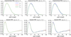 |
Fig. 2. Histograms for distribution of randomly generated path lengths, corresponding to different optical depth scales discussed in this paper. The model is described in Sect. 4.1, and the different columns correspond to different levels of initial linear polarisation. Top panels: optical depths randomly generated from an exponential distribution, bottom panels: optical depths generated by using the composite biasing approach discussed in Baes et al. (2016). |
However, it is not always advisable to randomly generate optical depths from an exponential distribution. One particularly relevant case is the penetration of radiation through an optically thick medium, which is a notoriously difficult task for Monte Carlo radiative transfer (e.g. Min et al. 2009; Gordon et al. 2017; Camps & Baes 2018). For a standard exponential PDF, huge numbers of photon packages need to be generated before a single one might cross the barrier. Path length stretching (Levitt 1968; Spanier 1970; Dwivedi 1982) is a Monte Carlo optimisation technique that artificially stimulates the generation of larger path lengths. Baes et al. (2016) combine this technique with the concept of composite biasing, which results in an approach that has the advantages of path length stretching (an increased probability for large path lengths) and minimises the disadvantages (no large weight factors for the photon packages). The bottom row of Fig. 2 shows the same histograms as the top row, but now the random optical depths are sampled from a biased distribution (for details, see Baes et al. 2016, Sect. 4.3). As the total optical depth is no longer guaranteed to be a good approximation for the dichroic optical depth at high optical depths, it is no surprise that the distributions are now more different, especially in the high path length tail. Kolmogorov–Smirnov (KS) tests indicate that the probability that they are drawn from the same distribution is negligible.
4.2. Practical calculation of the dichroic optical depth
The results from the previous subsections show that it is not a good idea to use the extinction or total optical depth scale to generate random path lengths in a Monte Carlo radiative transfer simulation with non-spherical dust grains. To avoid systematic errors, the dichroic optical depth scale should be used to translate randomly generated optical depths to physical path lengths. We hence need an efficient calculation for the dichroic optical depth τdic(s) along the path. However, in Sect. 3.3 we argue that it is not possible to write down a general closed formula for τdic(s), which is similar to the “simple” formulae (7) and (18) for the extinction and total optical depth scales, respectively. In general, a solution for τdic(s) needs to be obtained numerically using standard vector ODE solution techniques.
Fortunately, in the context of Monte Carlo radiative transfer simulations, in which the density of the medium is usually discretised on a grid with a uniform density and uniform optical properties within each grid cell, there is an efficient routine to solve the radiative transfer equation without the need for vector ODE solution methods (see also Whitney & Wolff 2002; Lucas 2003). Indeed, we can progressively solve the radiative transfer equation in each individual cell along the path. We assume again that the path is split into individual cells that are small enough so the density, optical properties, and grain orientation can be considered uniform within each cell. We denote the Stokes vector at the entry point of cell m as Im − 1. We first rotate the Stokes vector over an angle ψm to align it with the grain orientation within cell m,
 (27)
(27)
As the grain orientation with the cell is constant, we can directly apply the solution (21) for the radiative transfer to calculate the Stokes vector at the exit point s = sm of the cell,
![Mathematical equation: $$ \begin{aligned}&I_m^\prime = \mathrm{e}^{-\Delta \tau _{\mathrm{ext},m}} \left[I_{m-1}^\prime \cosh \Delta \tau _{\mathrm{pol},m} - Q_{m-1}^\prime \sinh \Delta \tau _{\mathrm{pol},m}\right],\end{aligned} $$](/articles/aa/full_html/2019/10/aa33796-18/aa33796-18-eq31.gif) (28)
(28)
![Mathematical equation: $$ \begin{aligned}&Q_m^\prime = \mathrm{e}^{-\Delta \tau _{\mathrm{ext},m}} \left[Q_{m-1}^\prime \cosh \Delta \tau _{\mathrm{pol},m} - I_{m-1}^\prime \sinh \Delta \tau _{\mathrm{pol},m}\right],\end{aligned} $$](/articles/aa/full_html/2019/10/aa33796-18/aa33796-18-eq32.gif) (29)
(29)
![Mathematical equation: $$ \begin{aligned}&U_m^\prime = \mathrm{e}^{-\Delta \tau _{\mathrm{ext},m}} \left[U_{m-1}^\prime \cos \Delta \tau _{\mathrm{cpol},m} - V_{m-1}^\prime \sin \Delta \tau _{\mathrm{cpol},m}\right],\end{aligned} $$](/articles/aa/full_html/2019/10/aa33796-18/aa33796-18-eq33.gif) (30)
(30)
![Mathematical equation: $$ \begin{aligned}&V_m^\prime = \mathrm{e}^{-\Delta \tau _{\mathrm{ext},m}} \left[V_{m-1}^\prime \cos \Delta \tau _{\mathrm{cpol},m} + U_{m-1}^\prime \sin \Delta \tau _{\mathrm{cpol},m}\right] , \end{aligned} $$](/articles/aa/full_html/2019/10/aa33796-18/aa33796-18-eq34.gif) (31)
(31)
and
 (32)
(32)
When we rotate the resulting Stokes vector back to the laboratory frame, we find the desired result Im,
 (33)
(33)
This recipe can be repeated for all cells along the path.
We tested this strategy using the same example as already discussed. The comparison between the brute-force Runge–Kutta approach and the algorithm described above is shown in Fig. 3 for an initially unpolarised Stokes vector. The top panel shows the evolution of the individual Stokes components, the bottom panels shows the Stokes ratios, as well as the degree of linear and total polarisation
 (34)
(34)
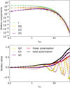 |
Fig. 3. Evolution of initially unpolarised Stokes vector propagating through medium of aligned grains where grain alignment rotates around path. The dots are the result from a Runge–Kutta numerical integration of the vector radiative transfer equation and the solid lines correspond to the method outlined in Sect. 3. |
The two methods clearly agree. As the initially unpolarised photon propagates along the path, it gradually develops linear polarisation as a result of dichroic extinction and also circular polarisation later on. From τ ≳ 8, the circular polarisation starts to dominate the linear polarisation, and at τ = 50, the photon is almost 100% polarised.
The determination of a random path length now follows the same strategy as discussed for the unpolarised Monte Carlo radiative transfer in Sect. 2. From the solution of the Stokes vector Im, we calculated the dichroic optical depth τdic, m at the exit point of each cell, and we searched for the first cell for which τdic, m exceeds the randomly determined τ. One additional difference needs to be taken into account. In the case of unpolarised radiation transfer, the increase in optical depth within each cell is directly proportional to the increase in path length within that cell, for example
 (35)
(35)
To find the exact path length s corresponding to a randomly generated τ, we can therefore use simple linear interpolation as follows:
 (36)
(36)
In the case of dichroic attenuation, the increase in optical depth within a cell is no longer proportional to the increase in path length, as
![Mathematical equation: $$ \begin{aligned} \tau _{\mathrm{dic}}(s)&= \tau _{\mathrm{dic},m-1}+n_m\,C_{\mathrm{ext},m}\,(s-s_{m-1}) \nonumber \\&\quad -\ln \,\Biggl [ \cosh \, \Bigl (n_m\,C_{\mathrm{pol},m}\,(s-s_{m-1})\Bigr ) \nonumber \\&\quad - \frac{Q_{m-1}^\prime }{I_{m-1}^\prime } \sinh \,\Bigl (n_m\,C_{\mathrm{pol},m}\,(s-s_{m-1})\Bigr ) \Biggr ] \nonumber \\&\quad \qquad \qquad \qquad \qquad {s_{m-1}\le s\le s_m.} \end{aligned} $$](/articles/aa/full_html/2019/10/aa33796-18/aa33796-18-eq40.gif) (37)
(37)
For a randomly generated τ, we should in principle use this equation to determine the correct value of s, which can be done using standard root-finding algorithms. In practice, however, we suggest using linear interpolation. Given the approximations due to the discretisation itself, the gain in accuracy by applying an exact root finding algorithm which is probably not worth the additional computational cost. Only in cases where the individual cells have a high optical depth could it possibly be useful to consider a more advanced, and numerically more costly, higher-order interpolation scheme.
One could argue that, in spite of the errors made, it would still be advantageous to use the extinction or total optical depth instead of the dichroic optical depth because the calculation of the dichroic optical depth is numerically more demanding. Indeed, calculating τext(s) or τtot(s) involves just a single summation along the path, whereas the calculation of τdic(s) requires the propagation of the entire Stokes vector, including rotations and hyperbolic function evaluations at every grid cell. However, it should be recognised that this operation has to be executed anyway in the Monte Carlo loop since the calculation of the Stokes vector up to the next interaction point is required. This is due to the albedo and the scattering matrix that explicitly depend on the polarisation state of the radiation (Mishchenko et al. 2000; Wolf et al. 2002). Rather than being a numerically expensive extra, the dichroic optical depth calculation is free. We can conclude that there is no benefit at all in using τext, τtot, or any other approximation, instead of the dichroic optical depth to calculate the next interaction location.
5. Summary and outlook
We have performed an analysis of the attenuation of radiation when it passes through a medium of aligned spheroidal grains, fully taking into account the effects of dichroism. The most important conclusions from this analysis are as follows.
Firstly, in a dichroic medium, the dichroic optical depth is no longer equivalent to the usual extinction optical depth τext, that is, the integral of the product of number density and extinction cross section along the path. For representative values of the optical properties of dust grains, the relative difference between both optical depth scales can be several tens of percent, even at low optical depths.
A potential option to account for dichroic attenuation could be to replace the extinction cross section by the total extinction cross section. The corresponding total optical depth τtot approximates the dichroic optical depth to first order, but it is always overestimated. Relative differences between total and dichroic optical depth are small at low optical depths, but they can also run up to several tens of percent at high optical depths. An accurate calculation of the dichroic optical depth requires the full solution of the intensity profile along the path. In the general case of a dichroic medium, the radiative transfer equation becomes a set of four coupled first-order differential equations with varying coefficients, and a closed expression for the dichroic optical depth cannot be derived. However, the exact solution corresponding to a medium with uniform grain alignment can be used to find the full solution in an elegant way without any further numerical integration. There is no benefit in using τext, τtot, or any other approximation instead of the dichroic optical depth to calculate the next interaction location in a Monte Carlo radiative transfer simulation.
Our results have implications for Monte Carlo radiative transfer coders that wish to incorporate the attenuation by elongated dust grains. If scattering polarisation by spherical grains already adds some complexity to Monte Carlo radiative transfer codes, dealing with non-spherical grains increases this complexity to a new level. Compared to spherical grains, the scattering process is significantly more complex. The scattering properties of spherical grains are fully described by just the albedo and the scattering phase function; for elongated grains, a full 4 × 4 scattering matrix comes into play (Mishchenko et al. 2000), and the random determination of a new propagation direction after a scattering event is not trivial (Wolf et al. 2002; Whitney & Wolff 2002; Lucas 2003). A related complexity concerns the amount of data that needs to be stored and accessed. Each of the elements of the extinction matrix and the scattering matrix is not only dependent on grain material, size, and wavelength, but also on shape and incidence angle. Moreover, each element of the scattering matrix needs to be discretised on the unit sphere. Finally, the process of dichroic extinction adds yet another level of complexity, and the results in this paper show that this also affects the random generation of the next interaction location.
So far, only a limited number of Monte Carlo radiative transfer codes have attempted to actually calculate dichroic attenuation by non-spherical aligned grains4. Wolf et al. (2002) were the first to include non-spherical aligned grains in their Monte Carlo radiative transfer calculations. They presented multiple light scattering calculations and demonstrated that the incorporation of elongated grains is important to explain the circular polarisation of light. They discussed the concepts of dichroism and birefringence, but they did not include these effects in the simulations they presented. Whitney & Wolff (2002) presented a Monte Carlo code that models the effects of scattering and dichroic absorption by aligned grains in circumstellar environments. While their code is presented for general geometries, they only discussed models with a uniform grain alignment. Simpson et al. (2013) applied this code to massive young stellar objects with more complex magnetic field configurations. Lucas (2003) presented a third Monte Carlo code with more or less the same characteristics as the code by Whitney & Wolff (2002), and also with the modelling of young stellar objects as the prime science objective. Applications of this code were presented by Lucas et al. (2004) and Chrysostomou et al. (2007). Peest et al. (in prep.) discuss the implementation of polarisation by elongated grains in the vectorised Monte Carlo code MC3D developed by (Krügel 2008; Heymann & Siebenmorgen 2012). Finally, a new Monte Carlo radiative transfer code, POLARIS, is presented by Reissl et al. (2016). It handles dichroic extinction and polarised emission, and it is optimised to handle data that results from sophisticated magneto-hydrodynamic simulations (Brauer et al. 2017; Reissl et al. 2017, 2018).
The work we present here fits into a broader effort to fully integrate the attenuation, polarisation, and thermal emission by elongated interstellar dust grains into the publicly available radiative transfer code SKIRT (Camps & Baes 2015). The advantage of implementing elongated grains in SKIRT is that the code can then use many of the useful ingredients that are already available, such as a suite of optimisation techniques (Baes et al. 2011, 2016), a library of input geometries for sources and sinks (Baes & Camps 2015), advanced spatial grids and grid traversal techniques (Camps et al. 2013; Saftly et al. 2013, 2014), the coupling to the output of grid-based and particle-based hydrodynamic codes (Saftly et al. 2015; Camps et al. 2016), and hybrid parallelisation techniques for shared and distributed memory machines (Verstocken et al. 2017).
Contrary to the currently available radiative transfer codes that incorporate elongated grains, SKIRT mainly focuses on galaxy-wide scales (e.g. De Looze et al. 2012, 2014; Viaene et al. 2017; Trayford et al. 2017). The magnetic and turbulent energy densities in nearby galaxies are found to be roughly in equipartition, and therefore magnetic fields are expected to be important for the evolution of galaxies (Boulares & Cox 1990; Beck et al. 1996). High-resolution cosmological zoom simulations have recently started to take magnetic fields into account (Pakmor et al. 2014, 2017; Grand et al. 2017). Radiative transfer codes that can fully incorporate dichroic extinction and emission by elongated aligned grains could be important tools to compare such simulations to observations.
Many of the quantities in this paper are dependent on wavelength, including the extinction cross section and the optical depth. In order not to overload the notations, we do not explicitly mention the wavelength dependence.
The MC3D radiative transfer code (Krügel 2008; Heymann & Siebenmorgen 2012) adopts an alternative method to find the next interaction point. For every dust cell along a path, they generate a new optical depth τ from an exponential distribution, and they compare this to the extinction optical depth Δτext, m within that cell. If τ < Δτext, m, the interaction position is determined by linear interpolation. Otherwise, the dust cell is crossed and the procedure is repeated for the next cell along the path. This methodology is equivalent to the method used by most of the other Monte Carlo codes, but it seems computationally more expensive and not straightforward to combine them with optimisation techniques as path length stretching (Levitt 1968; Spanier 1970; Baes et al. 2016) or forced scattering occurs (Cashwell & Everett 1959; Steinacker et al. 2013).
We can always perform a rotation to the initial Stokes vector to ensure that it is aligned with the grain orientation.
Several codes (Wood 1997; Wood & Jones 1997; Seon 2018) use an approximate treatment of dichroic attenuation, based on a non-linear relationship between the magnitude of dichroic polarisation and optical depth in our Milky Way (Jones 1989; Whittet et al. 2008).
References
- Aannestad, P. A., & Greenberg, J. M. 1983, ApJ, 272, 551 [NASA ADS] [CrossRef] [Google Scholar]
- Baes, M., & Camps, P. 2015, Astron. Comput., 12, 33 [NASA ADS] [CrossRef] [Google Scholar]
- Baes, M., Verstappen, J., De Looze, I., et al. 2011, ApJS, 196, 22 [NASA ADS] [CrossRef] [Google Scholar]
- Baes, M., Gordon, K. D., Lunttila, T., et al. 2016, A&A, 590, A55 [NASA ADS] [CrossRef] [EDP Sciences] [Google Scholar]
- Beck, R., Brandenburg, A., Moss, D., Shukurov, A., & Sokoloff, D. 1996, ARA&A, 34, 155 [NASA ADS] [CrossRef] [Google Scholar]
- Bianchi, S. 2008, A&A, 490, 461 [NASA ADS] [CrossRef] [EDP Sciences] [Google Scholar]
- Bianchi, S., Ferrara, A., & Giovanardi, C. 1996, ApJ, 465, 127 [NASA ADS] [CrossRef] [Google Scholar]
- Boulares, A., & Cox, D. P. 1990, ApJ, 365, 544 [NASA ADS] [CrossRef] [Google Scholar]
- Brauer, R., Wolf, S., Reissl, S., & Ober, F. 2017, A&A, 601, A90 [NASA ADS] [CrossRef] [EDP Sciences] [Google Scholar]
- Camps, P., & Baes, M. 2015, Astron. Comput., 9, 20 [NASA ADS] [CrossRef] [Google Scholar]
- Camps, P., & Baes, M. 2018, ApJ, 861, 80 [NASA ADS] [CrossRef] [Google Scholar]
- Camps, P., Baes, M., & Saftly, W. 2013, A&A, 560, A35 [NASA ADS] [CrossRef] [EDP Sciences] [Google Scholar]
- Camps, P., Trayford, J. W., Baes, M., et al. 2016, MNRAS, 462, 1057 [CrossRef] [Google Scholar]
- Cashwell, E., & Everett, C. 1959, A practical manual on the Monte Carlo method for random walk problems (Oxford: Pergamon Press) [Google Scholar]
- Chrysostomou, A., Lucas, P. W., & Hough, J. H. 2007, Nature, 450, 71 [NASA ADS] [CrossRef] [Google Scholar]
- Code, A. D., & Whitney, B. A. 1995, ApJ, 441, 400 [NASA ADS] [CrossRef] [Google Scholar]
- Davis, Jr., L., & Greenstein, J. L. 1951, ApJ, 114, 206 [Google Scholar]
- De Looze, I., Baes, M., Bendo, G. J., et al. 2012, MNRAS, 427, 2797 [NASA ADS] [CrossRef] [Google Scholar]
- De Looze, I., Fritz, J., Baes, M., et al. 2014, A&A, 571, A69 [NASA ADS] [CrossRef] [EDP Sciences] [Google Scholar]
- Dupree, S. A., & Fraley, S. K. 2002, A Monte Carlo Primer: A Practical Approach to Radiation Transport (Springer Science & Business Media) [CrossRef] [Google Scholar]
- Dwivedi, S. R. 1982, Ann. Nucl. Energy, 9, 359 [CrossRef] [Google Scholar]
- Ercolano, B., Barlow, M. J., Storey, P. J., & Liu, X.-W. 2003, MNRAS, 340, 1136 [NASA ADS] [CrossRef] [Google Scholar]
- Fischer, O., Henning, T., & Yorke, H. W. 1994, A&A, 284, 187 [NASA ADS] [Google Scholar]
- Gordon, K. D., Misselt, K. A., Witt, A. N., & Clayton, G. C. 2001, ApJ, 551, 269 [NASA ADS] [CrossRef] [Google Scholar]
- Gordon, K. D., Baes, M., Bianchi, S., et al. 2017, A&A, 603, A114 [NASA ADS] [CrossRef] [EDP Sciences] [Google Scholar]
- Grand, R. J. J., Gómez, F. A., Marinacci, F., et al. 2017, MNRAS, 467, 179 [NASA ADS] [Google Scholar]
- Heymann, F., & Siebenmorgen, R. 2012, ApJ, 751, 27 [NASA ADS] [CrossRef] [Google Scholar]
- Hovenier, J. W., & van der Mee, C. V. M. 1996, J. Quant. Spectr. Radiat. Transf., 55, 649 [NASA ADS] [CrossRef] [Google Scholar]
- Hubber, D. A., Ercolano, B., & Dale, J. 2016, MNRAS, 456, 756 [NASA ADS] [CrossRef] [Google Scholar]
- Jones, R. V., & Spitzer, Jr., L. 1967, ApJ, 147, 943 [NASA ADS] [CrossRef] [Google Scholar]
- Jones, T. J. 1989, ApJ, 346, 728 [NASA ADS] [CrossRef] [Google Scholar]
- Kalos, M. H., & Whitlock, P. A. 2008, Monte Carlo Methods: Second Revised and Enlarged Edition (Wiley-VCH Verlag) [CrossRef] [Google Scholar]
- Krügel, E. 2008, An Introduction to the Physics of Interstellar Dust (Taylor & Francis) [Google Scholar]
- Lazarian, A. 1994, MNRAS, 268, 713 [NASA ADS] [Google Scholar]
- Lazarian, A. 2007, J. Quant. Spectr. Radiat. Transf., 106, 225 [NASA ADS] [CrossRef] [Google Scholar]
- Levitt, L. B. 1968, Nucl. Sci. Eng., 31, 500 [CrossRef] [Google Scholar]
- Lucas, P. 2003, J. Quant. Spectr. Radiat. Transf., 79, 921 [NASA ADS] [CrossRef] [Google Scholar]
- Lucas, P. W., Fukagawa, M., Tamura, M., et al. 2004, MNRAS, 352, 1347 [NASA ADS] [CrossRef] [Google Scholar]
- Lunttila, T., & Juvela, M. 2012, A&A, 544, A52 [NASA ADS] [CrossRef] [EDP Sciences] [Google Scholar]
- Martin, P. G. 1972, MNRAS, 159, 179 [NASA ADS] [CrossRef] [Google Scholar]
- Martin, P. G. 1974, ApJ, 187, 461 [NASA ADS] [CrossRef] [Google Scholar]
- Min, M., Dullemond, C. P., Dominik, C., de Koter, A., & Hovenier, J. W. 2009, A&A, 497, 155 [NASA ADS] [CrossRef] [EDP Sciences] [Google Scholar]
- Mishchenko, M. I., Hovenier, J. W., & Travis, L. D. 2000, Light Scattering by Nonspherical Particles: Theory, Measurements, and Applications (San Diego: Academic Press) [Google Scholar]
- Niccolini, G., & Alcolea, J. 2006, A&A, 456, 1 [NASA ADS] [CrossRef] [EDP Sciences] [Google Scholar]
- Pakmor, R., Marinacci, F., & Springel, V. 2014, ApJ, 783, L20 [NASA ADS] [CrossRef] [Google Scholar]
- Pakmor, R., Gómez, F. A., Grand, R. J. J., et al. 2017, MNRAS, 469, 3185 [NASA ADS] [CrossRef] [Google Scholar]
- Peest, C., Camps, P., Stalevski, M., Baes, M., & Siebenmorgen, R. 2017, A&A, 601, A92 [NASA ADS] [CrossRef] [EDP Sciences] [Google Scholar]
- Reissl, S., Wolf, S., & Brauer, R. 2016, A&A, 593, A87 [NASA ADS] [CrossRef] [EDP Sciences] [Google Scholar]
- Reissl, S., Seifried, D., Wolf, S., Banerjee, R., & Klessen, R. S. 2017, A&A, 603, A71 [NASA ADS] [CrossRef] [EDP Sciences] [Google Scholar]
- Reissl, S., Klessen, R. S., Mac Low, M.-M., & Pellegrini, E. W. 2018, A&A, 611, A70 [NASA ADS] [CrossRef] [EDP Sciences] [Google Scholar]
- Robitaille, T. P. 2011, A&A, 536, A79 [NASA ADS] [CrossRef] [EDP Sciences] [Google Scholar]
- Saftly, W., Camps, P., Baes, M., et al. 2013, A&A, 554, A10 [NASA ADS] [CrossRef] [EDP Sciences] [Google Scholar]
- Saftly, W., Baes, M., & Camps, P. 2014, A&A, 561, A77 [NASA ADS] [CrossRef] [EDP Sciences] [Google Scholar]
- Saftly, W., Baes, M., De Geyter, G., et al. 2015, A&A, 576, A31 [NASA ADS] [CrossRef] [EDP Sciences] [Google Scholar]
- Seon, K.-I. 2018, ApJ, 862, 87 [NASA ADS] [CrossRef] [Google Scholar]
- Serkowski, K. 1962, Adv. Astron. Astrophys., 1, 289 [NASA ADS] [CrossRef] [Google Scholar]
- Simpson, J. P., Whitney, B. A., Hines, D. C., et al. 2013, MNRAS, 435, 3419 [NASA ADS] [CrossRef] [Google Scholar]
- Spanier, J. 1970, SIAM J. Appl. Math., 18, 172 [CrossRef] [Google Scholar]
- Steinacker, J., Baes, M., & Gordon, K. D. 2013, ARA&A, 51, 63 [NASA ADS] [CrossRef] [Google Scholar]
- Trayford, J. W., Camps, P., Theuns, T., et al. 2017, MNRAS, 470, 771 [NASA ADS] [CrossRef] [Google Scholar]
- van de Hulst, H. C. 1957, Light Scattering by Small Particles (New York: John Wiley & Sons) [Google Scholar]
- Verstocken, S., Van De Putte, D., Camps, P., & Baes, M. 2017, Astronomy and Computing, 20, 16 [Google Scholar]
- Viaene, S., Baes, M., Tamm, A., et al. 2017, A&A, 599, A64 [NASA ADS] [CrossRef] [EDP Sciences] [Google Scholar]
- Whitney, B. A. 2011, Bull. Astron. Soc. India, 39, 101 [NASA ADS] [Google Scholar]
- Whitney, B. A., & Wolff, M. J. 2002, ApJ, 574, 205 [NASA ADS] [CrossRef] [Google Scholar]
- Whitney, B. A., Robitaille, T. P., Bjorkman, J. E., et al. 2013, ApJS, 207, 30 [NASA ADS] [CrossRef] [Google Scholar]
- Whittet, D. C. B., Hough, J. H., Lazarian, A., & Hoang, T. 2008, ApJ, 674, 304 [NASA ADS] [CrossRef] [Google Scholar]
- Wolf, S., Voshchinnikov, N. V., & Henning, T. 2002, A&A, 385, 365 [NASA ADS] [CrossRef] [EDP Sciences] [Google Scholar]
- Wood, K. 1997, ApJ, 477, L25 [NASA ADS] [CrossRef] [Google Scholar]
- Wood, K., & Jones, T. J. 1997, AJ, 114, 1405 [NASA ADS] [CrossRef] [Google Scholar]
- Yajima, H., Li, Y., Zhu, Q., & Abel, T. 2012, MNRAS, 424, 884 [NASA ADS] [CrossRef] [Google Scholar]
All Figures
|
Fig. 1. Top left: relative differences δext between extinction optical depth τext and dichroic optical depth τdic for hypothetical example with density and grain alignment increasing linearly with increasing path length. The different curves correspond to different input Stokes vectors. In each case the photon package is initially fully linearly polarised, but the Stokes vector orientation θ increases in steps of 5°. The red lines corresponds to θ = 0° (Q0/I0 = 1) and the purple line to θ = 90° (Q0/I0 = −1), respectively. Bottom left: similar to top left panel, but now showing relative difference δtot between total optical depth τtot and dichroic optical depth. Right: same as panels on left, but now for model with uniform grain alignment. |
| In the text | |
|
Fig. 2. Histograms for distribution of randomly generated path lengths, corresponding to different optical depth scales discussed in this paper. The model is described in Sect. 4.1, and the different columns correspond to different levels of initial linear polarisation. Top panels: optical depths randomly generated from an exponential distribution, bottom panels: optical depths generated by using the composite biasing approach discussed in Baes et al. (2016). |
| In the text | |
|
Fig. 3. Evolution of initially unpolarised Stokes vector propagating through medium of aligned grains where grain alignment rotates around path. The dots are the result from a Runge–Kutta numerical integration of the vector radiative transfer equation and the solid lines correspond to the method outlined in Sect. 3. |
| In the text | |
Current usage metrics show cumulative count of Article Views (full-text article views including HTML views, PDF and ePub downloads, according to the available data) and Abstracts Views on Vision4Press platform.
Data correspond to usage on the plateform after 2015. The current usage metrics is available 48-96 hours after online publication and is updated daily on week days.
Initial download of the metrics may take a while.