| Issue |
A&A
Volume 629, September 2019
|
|
|---|---|---|
| Article Number | A100 | |
| Number of page(s) | 18 | |
| Section | Catalogs and data | |
| DOI | https://doi.org/10.1051/0004-6361/201936178 | |
| Published online | 11 September 2019 | |
MUSE library of stellar spectra⋆
1
European Southern Observatory, Karl-Schwarzschild-Str. 2, 85748 Garching bei München, Germany
e-mail: vivanov@eso.org
2
Dipartimento di Fisica e Astronomia “G. Galilei”, Université di Padova, Vicolo dell’Osservatorio 3, 35122 Padova, Italy
3
INAF-Osservatorio Astronomico di Padova, Vicolo dell’Osservatorio 5, 35122 Padova, Italy
4
European Southern Observatory, Ave. Alonso de Córdova 3107, Vitacura, Santiago, Chile
5
Instituto de Astronomía y Ciencias Planetarias Universidad de Atacama, Copiapó, Chile
Received:
25
June
2019
Accepted:
5
August
2019
Context. Empirical stellar spectral libraries have applications in both extragalactic and stellar studies, and they confer an advantage over theoretical libraries because they naturally include all relevant chemical species and physical processes. In recent years we have seen a stream of new sets of high-quality spectra, but increasing the spectral resolution and widening the wavelength coverage means resorting to multi-order echelle spectrographs. Assembling the spectra from many pieces results in lower fidelity of their shapes.
Aims. We aim to offer the community a library of high-signal-to-noise spectra with reliable continuum shapes. Furthermore, the use of an integral field unit (IFU) alleviates the issue of slit losses.
Methods. Our library was built with the MUSE (Multi-Unit Spectroscopic Explorer) IFU instrument. We obtained spectra over nearly the entire visual band (λ ∼ 4800–9300 Å).
Results. We assembled a library of 35 high-quality MUSE spectra for a subset of the stars from the X-shooter Spectral Library. We verified the continuum shape of these spectra with synthetic broadband colors derived from the spectra. We also report some spectral indices from the Lick system, derived from the new observations.
Conclusions. We offer a high-fidelity set of stellar spectra covering the Hertzsprung-Russell diagram. These can be used for both extragalactic and stellar studies and demonstrate that the IFUs are excellent tools for building reliable spectral libraries.
Key words: standards / atlases / stars: atmospheres / stars: general
The spectra (full Table A.2) are only available at the CDS via anonymous ftp to cdsarc.u-strasbg.fr (130.79.128.5) or via http://cdsarc.u-strasbg.fr/viz-bin/cat/J/A+A/629/A100
© ESO 2019
1. Introduction
Empirical stellar spectral libraries are one of the most universally applicable tools in modern astronomy. They have applications in both extragalactic and stellar studies. The former include the modelling of unresolved stellar populations (e.g., Röck et al. 2016), matching and removing continua to reveal weak emission lines (e.g., Engelbracht et al. 1998), and use as templates to measure the stellar line-of-sight velocity dispersions in galaxies (Sargent et al. 1977; Krajnović et al. 2015; Johnston et al. 2018; Martinsson et al. 2018; Nedelchev et al. 2019). The stellar applications include measuring stellar parameters such as effective temperatures (e.g., Beamín et al. 2015) and surface gravities (e.g., Terrien et al. 2015) by template matching or indices, measuring radial velocities (e.g., Swan et al. 2016), and verifying theoretical stellar models which are sometimes not as good as one may expect. For example, Sansom et al. (2013) found discrepancies in the Balmer lines, suggesting that the theoretical spectral libraries may not be as reliable a source of stellar spectra as the empirical ones. The lists of applications given here are by far incomplete.
We can add a number of open issues related to the libraries. First, the need to derive homogeneous and self-consistent stellar parameters of the library stars. Currently, the stellar parameters are typically assembled from multiple sources, which requires a two-step process: first, global solutions of stellar parameters Teff/[Fe/H]/logg must be derived from spectral indices, and then these relations must be inverted before deriving a new, uniform set of stellar parameters for all stars (e.g., Sharma et al. 2016; Arentsen et al. 2019). Another issue is to define optimal indices that are sensitive to one or another stellar parameter (e.g., Cesetti et al. 2013). A particular problem related to galaxy models is the contribution of the AGB stars (e.g., Maraston 2005).
The most widely used theoretical libraries today are the BaSeL (Kurucz 1992; Lejeune et al. 1997, 1998; Westera et al. 2002) and the PHOENIX (Hauschildt et al. 1999; Allard et al. 2012; Husser et al. 2013) libraries, but there have been problems with the treatment of molecules, as shown early on by Castelli et al. (1997), that occasionally lead to poorly predicted broadband colors. Among the empirical libraries, the work of Pickles (1998) was the most widely used. It includes 131 flux-calibrated stars, but for the vast majority of them the resolving power was below R = 1000, which is relatively low even for extragalactic applications where the intrinsic velocity dispersion of galaxies requires R ∼ 2000 or higher. Other sets of spectra of better quality have become available, such as ELODIE (Soubiran et al. 1998; Prugniel & Soubiran 2001; Le Borgne et al. 2004), STELIB (Le Borgne et al. 2003), Indo-US (Valdes et al. 2004), MILES (Sánchez-Blázquez et al. 2006), and CaT (Cenarro et al. 2001, 2007). More recently, a single-order library with a large number of stars was reported by Yan et al. (2018), but this was obtained with a 3 arcsec fiber of the SDSS spectrograph (Blanton et al. 2017) and therefore does not completely avoid the slit-loss problem. Maraston & Strömbäck (2011) incorporated some of the libraries listed here into a comprehensive stellar population model at high spectral resolution.
The X-shooter Spectral Library (XSL; Chen et al. 2014) is the latest and most comprehensive effort in this direction. At this time only Data Release 1 with optical spectra of 237 stars is available. When completed, XSL will cover the 0.3–2.5 μm range at a resolving power of R∼7000–11 000. This library showcases the problems that increasing resolution and multi-order cross-dispersed spectrographs bring in: the synthetic broadband optical (UBV) colors agree poorly with the observed colors from the Bright Star Catalog (on average at ∼7% level; see Table 5 and Fig. 26 in Chen et al. 2014). The differences are partially related to pulsating variable stars having been observed in different phases. Slit losses are another issue; for many stars these are caused by the lack or poor quality of wide slit observations. Despite these problems, the narrow features in the XSL spectra are self-consistent; for example observations in different orders agree well (see Fig. 8 in Chen et al. 2014), and there is good agreement between features and theoretical models and other empirical libraries (for a comparison with the UVES-POP, see Figs. 31–34 in Chen et al. 2014).
In other words, we are again facing a familiar problem: the old theoretical libraries used to predict colors that were inconsistent with the observations; nowadays, the newest empirical libraries do the same, despite – or because of – the excellent quality of the new data, which made it more apparent. To address this issue, we embarked on a project to build an empirical spectral library without slit loss, using the MUSE (Multi-Unit Spectroscopic Explorer; Bacon et al. 2010) integral field unit, spanning all major sequences on the Hertzsprung-Russell diagram, with the specific goal of adjusting and verifying the shapes of the spectra in other libraries, both theoretical and empirical. The final products are spectra that are suitable for galactic modeling, stellar classification, and other applications. Here we report the first subset of 35 MUSE stellar spectra.
The following two sections describe the sample and the data, respectively. Section 4 presents the analysis of our spectra and Sect. 5 summarizes this work.
2. Sample
Our initial sample numbered 33 targets selected among the XSL stars1. We aimed to populate the Hertzsprung-Russell diagram as homogeneously as possible with ∼3–6 bright stars per spectral type, ensuring a high signal-to-noise ratio (S/N)> 70–200 per spectral type, except for the O-type where only a single star was available.
Spectra of two additional stars were obtained: HD 193256 and HD 193281B. They serendipitously fell inside the field of view during the observations of the project target HD 193281A. An IFU campaign covering the entire XSL is planned, but we made sure to select stars over various spectral types, making this trimmed-down library adequate for some applications, such as stellar classification and template-fitting of galaxy spectra.
The SIMBAD spectral types as listed in Chen et al. (2014), and complemented for the two extra targets, together with effective temperatures Teff, surface gravities logg, and metallicities [Fe/H] collected from the literature, if available, are listed in Table 1 and shown in Fig. 1 2. The covered range of Teff is 2600−33 000 K, of logg: 0.6−4.5 and of [Fe/H]: from −1.22 to 0.55, as far as the stellar parameters are known. In cases where multiple literature sources with equal quality were available for a certain parameter, we adopted the average value and if a given source had significantly smaller errors than the others, we adopted the value from that source.
Physical parameters of the program stars.
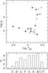 |
Fig. 1. Properties of the stars in our sample. Top: surface gravity logg vs. effective temperature Teff for stars with [Fe/H] ≤ −0.5 dex (crosses), −0.5 < [Fe/H] < 0.0 dex (open circles), and [Fe/H] ≥ 0.0 dex (solid dots). Bottom: distributions of the stars by spectral type. |
3. Observations and data reduction
The spectra were obtained with MUSE at the European Southern Observatory (ESO) Very Large Telescope, Unit Telescope 4, on Cerro Paranal, Chile. Table A.1 gives the observing log. We obtained six exposures for each target, except for HD 204155 which was observed 12 times. To maximize the data yield, most of the data were obtained under nonphotometric conditions, so the absolute flux calibration is uncertain, but the “true” intrinsic shape is preserved, because there is no “stitching” of multiple orders and no variable slit losses due to atmospheric refraction. We placed the science targets at the same spaxels as the spectrophotometric standards to minimize the instrument systematic error that might arise from residual spaxel-to-spaxel variations.
Data reduction was performed with the ESO MUSE pipeline (version 2.6) within the ESO Reflex3 environment (Freudling et al. 2013). The 1D spectra were extracted within a circular aperture with a radius of 6 arcsec. This number was selected after some experiments with apertures of difference sizes, to guarantee that “aperture” losses lead to a change in the overall slope of the spectra < 1% from the blue to the red end. The sky emission was estimated within an annulus of an inner radius of 7 arcsec and a width of 4 arcsec. This step of the analysis was performed with an IRAF4/PyRAF tool (Tody 1986, 1993; Science Software Branch at STScI 2012).
Three stars were treated differently. For [B86] 133 we reduced the extraction aperture radius to 4 arcsec (keeping the sky annulus the same as for the majority of the targets) to avoid contamination from nearby sources – because the object is located in a crowded Milky Way bulge field. HD 193256 is close to the edge of the MUSE field of view, and the extraction apertures had to be smaller, with a radius 4.6 arcsec, the sky annulus had an inner radius of 4.6 arcsec and a width of 2 arcsec. HD 193281 is a binary with ∼3.8 arcsec separation and the components cross-contaminate each other. To separate the two spectra we first extracted a combined spectrum of the two stars together with the same aperture and annulus as for the bulk of the stars. We then rotated each plane of the data cube by 180° around the center of the primary and subtracted the rotated plane from the original nonrotated plane to remove the contribution of the primary at the location of the secondary. Subsequently, we extracted the spectrum of the secondary with an aperture with a radius of 1.2 arcsec and a sky annulus with an inner radius of 1.8 arcsec and a width of 4 arcsec. Finally, we decontaminated the spectrum of the primary by subtracting the spectrum of the secondary from the combined spectrum of the binary.
Experiments with apertures of different sizes indicated that the continuum shape of [B86] 133 still changed at < 1% level across the entire wavelength range, despite the narrower extraction aperture. The spectra of the two other objects are less reliable and in the case of HD 193281B a change in the radius of a few spaxels (0.2 arcsec) leads to a flux change of ∼3% over the entire wavelength range. However, the spectrum of HD 193281A is still stable at < 1% because the secondary contributes ∼1 and ∼11% to the total flux at the blue and at the red ends of the spectrum, respectively, so this ∼3% uncertainty is reduced by factors of ∼100 and ∼9, respectively, and the spectrum of HD 193281A can be considered reliable according to our criterion for < 1% stability across the entire spectral range.
The telluric features were removed by running molecfit version 1.5.7 (Smette et al. 2015; Kausch et al. 2015) separately on each of the six (12 for HD 204155) target spectra themselves. The agreement of individual solutions is excellent: typically the fits yield a precipitable water estimate identical to within < 0.1 mm.
The final spectrum for each target is the average of the 1D spectra derived from the six individual observations, and the error is the rms of that average. An example of the data products is plotted in Fig. 2. The complete sample is shown in Fig. A.1. All final spectra are given in Table A.2 and are available at the CDS.
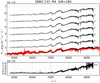 |
Fig. 2. Example of the MUSE spectra (black line) of [B86] 133 and of the corresponding XSL DR1 spectrum (red line; normalized to match the MUSE spectrum flux). The plot title lists the spectral type and the measured median S/N per resolution element over the entire spectrum. Upper sub-panels: spectra extracted from each individual exposure (shifted up for clarity) and average spectra of the object at its true flux level. Bottom sub-panels: standard deviation of the average spectrum. The spectra of the other sample stars are presented in Fig. A.1. |
4. Analysis
A direct comparison of the MUSE and XSL spectra for eight randomly selected stars across the spectral type sequence is shown with some zoomed-in spectral regions in Fig. 3 (for the rest of our spectra, see Figs. 2 and A.1). Notably, the XSL spectra used the continuum shape from 5 arcsec wide-slit observations. In most cases, the agreement on a scale of a few hundred pixels – in other words, within the same X-shooter order – is excellent. However, on a wider scale we find deviations between the XSL and MUSE spectra, as can be seen in Fig. 4. The exceptions are usually late-type stars – [B86] 133 and IRAS 15060+0947 are examples – where the low S/N in the blue (∼10 or below) and the variability that only occurs with extremely red stars may account for the problem. Furthermore, the ratios of many spectra show a gradual change, despite their apparently high S/N: HD 147550 and HD 167278 are examples where the amplitude of the ratio within the MUSE wavelength range reaches 10−15%. We fitted second-order polynomials to the ratios and extrapolated them over the full wavelength range covered by the XSL library to demonstrate that if these trends hold, the overall peak-to-peak flux differences can easily rich ∼20%, meaning that the overall continuum of the cross-dispersed spectra is somewhat ill-defined. The coefficients of the polynomial fits are listed in Table B.1 and can be used to correct the shape of the XSL spectra. We are far from critisizing Chen et al. (2014) for the quality of their data reduction; rather we point out here that the high-S/N observations show how difficult it is to process cross-dispersed spectra. Indeed, problems that may not be obvious with poor-quality data become apparent for S/Ns of 100−200.
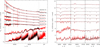 |
Fig. 3. Comparison of a subset of our MUSE spectra (black lines) with the XSL spectra (red lines; boxcar smoothed over 8 pixels). The spectra are normalized to unity between the two vertical dotted lines shown on the left panel, and shifted vertically for display purposes. Left panel: entire MUSE spectral range, right panel: zoom onto the Hβ, Hα, and Ca triplet wavelength ranges (left to right). No radial velocity corrections are applied. |
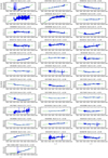 |
Fig. 4. Ratios of the XSL spectra to our MUSE spectra (blue; covers only the MUSE wavelength range), normalized to unity and median smoothed for display purposes with a five-element wide median filter. Two ratios are shown for HD 101712 – for the two XSL spectra of this star. A second-order polynomial fit spanning the wavelength of XSL is also shown in blue. The labels on the top of each panel contain the name of the object, the normalization factor that indicates the flux ratio of the independently flux-calibrated MUSE and XSL spectra, and a standard deviation of the residuals of the fit. The coefficients of polynomial fits are listed in Table B.1. |
The question remains, however, as to whether or not the MUSE spectra have a more reliable shape than the XSL spectra, because strictly speaking so far we have only demonstrated the good internal agreement between the six (or 12) individual MUSE observations. To provide an external check we followed Chen et al. (2014), and calculated synthetic SDSS colors from both ours and the XSL spectra (Fig. 5) using the pyphot tool5. The XSL spectra were median smoothed to remove outliers, for example those due to poorly removed cosmic ray hits. The MUSE sequences are slightly tighter than the XSL ones, confirming that the MUSE spectra have more reliable shapes. This is expected in light of the slit losses and the imperfect order stitching of the XSL spectra. Furthermore, X-shooter has three arms – in effect, three different instruments, and some of the colors mix fluxes from different arms, which may contribute to the larger scatter. A better spectral shape verification will be possible in the future with the Gaia low-resolution spectra.
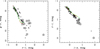 |
Fig. 5. Synthetic SDSS color-color diagrams derived from the MUSE (open circles) and XSL (open triangles) spectra. Larger open circles mark known variables, according to the SIMBAD database. and although many stars are variable, some distinct outliers are not. Sequences for solar abundance dwarfs (red line) and giant (green line) stars from Lenz et al. (1998) are also shown. The extreme red outliers are IRAS 15060+0947 (V* FV Boo) – a known Mira variable. There are two points for this object on the right panel – they correspond to the XSL and the MUSE spectra. |
The Lick indices (Worthey et al. 1994) that fall within the wavelength range covered by MUSE were measured in the new spectra (Table C.1). This included: Fe5015, Fe5270, Fe5335, Fe5406, Fe5709, Fe5782, Hβ, Mg1, Mg2, Mg b, Na D, TiO1 and TiO2. As designed by our target selection, the measured values occupy the same locus as the Lick library (Fig. 6).
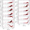 |
Fig. 6. Lick indices for the stars in our sample (red dots) and in the sample of Worthey et al. (1994, black dots). Following their definitions, Mg1, Mg2, TiO1 and TiO2 are in magnitudes, and the rest are equivalent widths in units of Å. The two coldest objects that often deviate from the M-star-dominated sequences are the carbon stars HD 067507 and HD 085405. |
In the course of the analysis we noticed that the Lick indices of HD 193281B correspond to a later type than the F5:V: reported in Simbad. We derived a new spectral type of K2III using our spectra of HD 170820 and HD 099998 as templates and we adopted for this star the average of their effective temperatures, Teff = 4354 K, with a tentative uncertainty of 57 K – the larger of the uncertainties of the Teff for these two stars.
The metal features of HD 179821 are stronger than for other stars with similar temperature, but this is probably due to the supersolar abundance of this star (Soubiran et al. 2016). Some Lick indices of late-M and C/S stars also deviate from the locus, but the spectra of these stars are dominated by broad molecular features, making the atomic indices, such as Fe, Mg, and H, meaningless.
5. Summary and conclusions
We present high-S/N (> 70–200) MUSE spectra of 35 stars across the spectral type sequence. The comparison with existing higher-resolution data and spectral index measurements shows reasonably good agreement, except for differences in the continuum shape that point out the real difficulties in obtaining high-resolution spectra with wide spectral coverage: the instruments that deliver such data spread the light over many orders and their combination is not trivial. Importantly, the integral field unit that we use does not suffer from slit losses.
The sample of spectra presented here is relatively limited in terms of number of stars, and to make this library more useful we need to populate the parametric space more densely. In particular, the metallicity range needs to be expanded. Our data suffer from the high blue wavelength limit of MUSE, missing some important CN, Ca, and Fe spectral features in the 4100–4800 Å range. This is a hardware limitation that can only be addressed with other/future instruments. Further accurate broadband photometry is needed to extend the external verification of the continuum shape – so far Gaia, SDSS, and other photometric surveys provide measurements only for about a quarter of our sample stars – mostly because our program stars are too bright. Expanding the MUSE library towards fainter stars will increase this fraction and make such a test statistically significant.
Despite these issues, our MUSE spectral library is a potentially useful tool for both stellar and galaxy research. This project started as a simple effort to complement the SXL DR1 library, but our spectra can be applied to various MUSE-based research projects – they confer the extra advantage of being obtained with the same instrument, meaning the data format is the same, and any low-level instrumental signatures that might have remained in the data could cancel out. We plan to expand the number of library stars in the future.
Stellar parameters from XSL also became available after the submission of this paper: Arentsen et al. (2019).
Acknowledgments
This paper is based on observations made with the ESO Very Large Telescope at the La Silla Paranal Observatory under program 099.D-0623. We have made extensive use of the SIMBAD Database at CDS (Centre de Données astronomiques) Strasbourg and of the VizieR catalog access tool, CDS, Strasbourg, France. E.M.C., E.D.B., L.M., and A.P. acknowledge financial support from Padua University through grants DOR1715817/17, DOR1885254/18, DOR1935272/19, and BIRD164402/16. We thank the referee for the comments that helped to improve the paper.
References
- Allard, F., Homeier, D., & Freytag, B. 2012, Trans. R. Soc. London Ser. A, 370, 2765 [NASA ADS] [Google Scholar]
- Ammons, S. M., Robinson, S. E., Strader, J., et al. 2006, ApJ, 638, 1004 [NASA ADS] [CrossRef] [Google Scholar]
- Arentsen, A., Prugniel, P., Gonneau, A., et al. 2019, A&A, 627, A138 [NASA ADS] [CrossRef] [EDP Sciences] [Google Scholar]
- Bacon, R., Accardo, M., Adjali, L., et al. 2010, in Ground-based and Airborne Instrumentation for Astronomy III, Proc. SPIE, 7735, 773508 [CrossRef] [Google Scholar]
- Beamín, J. C., Ivanov, V. D., Minniti, D., et al. 2015, MNRAS, 454, 4054 [NASA ADS] [CrossRef] [Google Scholar]
- Bergeat, J., Knapik, A., & Rutily, B. 2002, A&A, 390, 967 [NASA ADS] [CrossRef] [EDP Sciences] [Google Scholar]
- Blanton, M. R., Bershady, M. A., Abolfathi, B., et al. 2017, AJ, 154, 28 [NASA ADS] [CrossRef] [Google Scholar]
- Castelli, F., Gratton, R. G., & Kurucz, R. L. 1997, A&A, 318, 841 [NASA ADS] [Google Scholar]
- Cenarro, A. J., Cardiel, N., Gorgas, J., et al. 2001, MNRAS, 326, 959 [NASA ADS] [CrossRef] [Google Scholar]
- Cenarro, A. J., Peletier, R. F., Sánchez-Blázquez, P., et al. 2007, MNRAS, 374, 664 [NASA ADS] [CrossRef] [Google Scholar]
- Cesetti, M., Pizzella, A., Ivanov, V. D., et al. 2013, A&A, 549, A129 [NASA ADS] [CrossRef] [EDP Sciences] [Google Scholar]
- Chen, Y.-P., Trager, S. C., Peletier, R. F., et al. 2014, A&A, 565, A117 [NASA ADS] [CrossRef] [EDP Sciences] [Google Scholar]
- Engelbracht, C. W., Rieke, M. J., Rieke, G. H., Kelly, D. M., & Achtermann, J. M. 1998, ApJ, 505, 639 [NASA ADS] [CrossRef] [Google Scholar]
- Engels, D., & Bunzel, F. 2015, A&A, 582, A68 [NASA ADS] [CrossRef] [EDP Sciences] [Google Scholar]
- Famaey, B., Pourbaix, D., Frankowski, A., et al. 2009, A&A, 498, 627 [NASA ADS] [CrossRef] [EDP Sciences] [Google Scholar]
- Freudling, W., Romaniello, M., Bramich, D. M., et al. 2013, A&A, 559, A96 [NASA ADS] [CrossRef] [EDP Sciences] [Google Scholar]
- Gaia Collaboration 2018a, VizieR Online Data Catalog: I/345 [Google Scholar]
- Gaia Collaboration (Brown, A. G. A., et al.) 2018b, A&A, 616, A1 [NASA ADS] [CrossRef] [EDP Sciences] [Google Scholar]
- Gontcharov, G. A. 2006, Astron. Lett., 32, 759 [NASA ADS] [CrossRef] [Google Scholar]
- Hauschildt, P. H., Allard, F., Ferguson, J., Baron, E., & Alexander, D. R. 1999, ApJ, 525, 871 [NASA ADS] [CrossRef] [Google Scholar]
- Husser, T. O., Wende-von Berg, S., Dreizler, S., et al. 2013, A&A, 553, A6 [NASA ADS] [CrossRef] [EDP Sciences] [Google Scholar]
- Ivanov, V. D., Rieke, M. J., Engelbracht, C. W., et al. 2004, ApJS, 151, 387 [NASA ADS] [CrossRef] [Google Scholar]
- Johnston, E. J., Hau, G. K. T., Coccato, L., & Herrera, C. 2018, MNRAS, 480, 3215 [NASA ADS] [CrossRef] [Google Scholar]
- Kausch, W., Noll, S., Smette, A., et al. 2015, A&A, 576, A78 [NASA ADS] [CrossRef] [EDP Sciences] [Google Scholar]
- Koleva, M., & Vazdekis, A. 2012, A&A, 538, A143 [NASA ADS] [CrossRef] [EDP Sciences] [Google Scholar]
- Krajnović, D., Weilbacher, P. M., Urrutia, T., et al. 2015, MNRAS, 452, 2 [NASA ADS] [CrossRef] [Google Scholar]
- Kunder, A., Kordopatis, G., Steinmetz, M., et al. 2017, AJ, 153, 75 [NASA ADS] [CrossRef] [Google Scholar]
- Kurucz, R. L. 1992, in The Stellar Populations of Galaxies, eds. B. Barbuy, & A. Renzini, IAU Symp., 149, 225 [NASA ADS] [CrossRef] [Google Scholar]
- Latham, D. W., Stefanik, R. P., Torres, G., et al. 2002, AJ, 124, 1144 [NASA ADS] [CrossRef] [Google Scholar]
- Le Borgne, J.-F., Bruzual, G., Pelló, R., et al. 2003, A&A, 402, 433 [NASA ADS] [CrossRef] [EDP Sciences] [Google Scholar]
- Le Borgne, D., Rocca-Volmerange, B., Prugniel, P., et al. 2004, A&A, 425, 881 [NASA ADS] [CrossRef] [EDP Sciences] [Google Scholar]
- Lejeune, T., Cuisinier, F., & Buser, R. 1997, A&AS, 125, 229 [NASA ADS] [CrossRef] [EDP Sciences] [Google Scholar]
- Lejeune, T., Cuisinier, F., & Buser, R. 1998, A&AS, 130, 65 [NASA ADS] [CrossRef] [EDP Sciences] [Google Scholar]
- Lenz, D. D., Newberg, J., Rosner, R., Richards, G. T., & Stoughton, C. 1998, ApJS, 119, 121 [NASA ADS] [CrossRef] [MathSciNet] [Google Scholar]
- Maraston, C. 2005, MNRAS, 362, 799 [NASA ADS] [CrossRef] [Google Scholar]
- Maraston, C., & Strömbäck, G. 2011, MNRAS, 418, 2785 [NASA ADS] [CrossRef] [Google Scholar]
- Martinsson, T. P. K., Sarzi, M., Knapen, J. H., et al. 2018, A&A, 612, A66 [NASA ADS] [CrossRef] [EDP Sciences] [Google Scholar]
- Massarotti, A., Latham, D. W., Stefanik, R. P., & Fogel, J. 2008, AJ, 135, 209 [NASA ADS] [CrossRef] [Google Scholar]
- Mermilliod, J. C., Mayor, M., & Udry, S. 2008, A&A, 485, 303 [NASA ADS] [CrossRef] [EDP Sciences] [Google Scholar]
- Nedelchev, B., Coccato, L., Corsini, E. M., et al. 2019, A&A, 623, A87 [NASA ADS] [CrossRef] [EDP Sciences] [Google Scholar]
- Pickles, A. J. 1998, PASP, 110, 863 [CrossRef] [Google Scholar]
- Pourbaix, D., Tokovinin, A. A., Batten, A. H., et al. 2004, A&A, 424, 727 [NASA ADS] [CrossRef] [EDP Sciences] [Google Scholar]
- Prugniel, P., & Soubiran, C. 2001, A&A, 369, 1048 [NASA ADS] [CrossRef] [EDP Sciences] [Google Scholar]
- Prugniel, P., Vauglin, I., & Koleva, M. 2011, A&A, 531, A165 [NASA ADS] [CrossRef] [EDP Sciences] [Google Scholar]
- Röck, B., Vazdekis, A., Ricciardelli, E., et al. 2016, A&A, 589, A73 [NASA ADS] [CrossRef] [EDP Sciences] [Google Scholar]
- Sánchez-Blázquez, P., Peletier, R. F., Jiménez-Vicente, J., et al. 2006, MNRAS, 371, 703 [NASA ADS] [CrossRef] [Google Scholar]
- Sansom, A. E., Milone, A. D. C., Vazdekis, A., & Sánchez-Blázquez, P. 2013, MNRAS, 435, 952 [NASA ADS] [CrossRef] [Google Scholar]
- Santos, N. C., Mayor, M., Bonfils, X., et al. 2011, A&A, 526, A112 [NASA ADS] [CrossRef] [EDP Sciences] [Google Scholar]
- Sargent, W. L. W., Schechter, P. L., Boksenberg, A., & Shortridge, K. 1977, ApJ, 212, 326 [NASA ADS] [CrossRef] [Google Scholar]
- Science Software Branch at STScI 2012, Astrophysics Source Code Library [record ascl:1207.011] [Google Scholar]
- Sharma, K., Prugniel, P., & Singh, H. P. 2016, A&A, 585, A64 [NASA ADS] [CrossRef] [EDP Sciences] [Google Scholar]
- Smette, A., Sana, H., Noll, S., et al. 2015, A&A, 576, A77 [NASA ADS] [CrossRef] [EDP Sciences] [Google Scholar]
- Soubiran, C., Katz, D., & Cayrel, R. 1998, A&AS, 133, 221 [NASA ADS] [CrossRef] [EDP Sciences] [Google Scholar]
- Soubiran, C., Bienaymé, O., Mishenina, T. V., & Kovtyukh, V. V. 2008, A&A, 480, 91 [NASA ADS] [CrossRef] [EDP Sciences] [Google Scholar]
- Soubiran, C., Jasniewicz, G., Chemin, L., et al. 2013, A&A, 552, A64 [NASA ADS] [CrossRef] [EDP Sciences] [Google Scholar]
- Soubiran, C., Le Campion, J.-F., Brouillet, N., & Chemin, L. 2016, A&A, 591, A118 [NASA ADS] [CrossRef] [EDP Sciences] [Google Scholar]
- Swan, J., Cole, A. A., Tolstoy, E., & Irwin, M. J. 2016, MNRAS, 456, 4315 [NASA ADS] [CrossRef] [Google Scholar]
- Terrien, R. C., Mahadevan, S., Bender, C. F., Deshpande, R., & Robertson, P. 2015, ApJ, 802, L10 [NASA ADS] [CrossRef] [Google Scholar]
- Tody, D. 1986, in Instrumentation in Astronomy VI, ed. D. L. Crawford, Proc. SPIE, 627, 733 [NASA ADS] [CrossRef] [Google Scholar]
- Tody, D. 1993, in Astronomical Data Analysis Software and Systems II, eds. R. J. Hanisch, R. J. V. Brissenden, & J. Barnes, ASP Conf. Ser., 52, 173 [NASA ADS] [Google Scholar]
- Valdes, F., Gupta, R., Rose, J. A., Singh, H. P., & Bell, D. J. 2004, ApJS, 152, 251 [NASA ADS] [CrossRef] [Google Scholar]
- Westera, P., Lejeune, T., Buser, R., Cuisinier, F., & Bruzual, G. 2002, A&A, 381, 524 [NASA ADS] [CrossRef] [EDP Sciences] [Google Scholar]
- Wilson, R. E. 1953, General Catalogue of Stellar Radial Velocities (Washington: Carnegie Institution of Washington) [Google Scholar]
- Worthey, G., Faber, S. M., Gonzalez, J. J., & Burstein, D. 1994, ApJS, 94, 687 [NASA ADS] [CrossRef] [Google Scholar]
- Wright, C. O., Egan, M. P., Kraemer, K. E., & Price, S. D. 2003, AJ, 125, 359 [NASA ADS] [CrossRef] [Google Scholar]
- Yan, R., Chen, Y., Lazarz, D., et al. 2018, ApJ, submitted [arXiv:1812.02745] [Google Scholar]
Appendix A: MUSE spectra
Table A.1 presents the log of our MUSE observations and Fig. A.1 – the MUSE spectra.
Observing log.
MUSE spectra of the program stars.
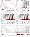 |
Fig. A.1. MUSE spectra (labeled on the top of each panel). Upper sub-panels: spectra extracted from each individual exposure (shifted up for clarity) and the average spectra of the object at its true flux level. The XSL spectra, when available, are plotted in red underneath the averaged MUSE spectrum. Bottom sub-panels: standard deviation of the average spectrum. The spectra of all stars are available at the CDS. |
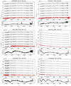 |
Fig. A.1. continued. |
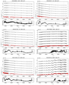 |
Fig. A.1. continued. |
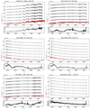 |
Fig. A.1. continued. |
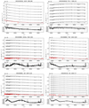 |
Fig. A.1. continued. |
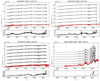 |
Fig. A.1. continued. |
Appendix B: Comparison with the XSL spectra
Table B.1 lists the coefficients of polynomial fits to the ratios of the XSL spectra to our MUSE spectra. For further details see Sect. 4.
Coefficients and their errors of second-order polynomial fits to the ratios of the XSL spectra to our MUSE spectra: Ratio = a0 + a1 × λ + a2 × λ2.
Appendix C: Lick indices from the MUSE spectra
Table C.1 shows the Lick indices measured on our MUSE spectra.
Lick indices measured on the MUSE spectra.
All Tables
Coefficients and their errors of second-order polynomial fits to the ratios of the XSL spectra to our MUSE spectra: Ratio = a0 + a1 × λ + a2 × λ2.
All Figures
|
Fig. 1. Properties of the stars in our sample. Top: surface gravity logg vs. effective temperature Teff for stars with [Fe/H] ≤ −0.5 dex (crosses), −0.5 < [Fe/H] < 0.0 dex (open circles), and [Fe/H] ≥ 0.0 dex (solid dots). Bottom: distributions of the stars by spectral type. |
| In the text | |
|
Fig. 2. Example of the MUSE spectra (black line) of [B86] 133 and of the corresponding XSL DR1 spectrum (red line; normalized to match the MUSE spectrum flux). The plot title lists the spectral type and the measured median S/N per resolution element over the entire spectrum. Upper sub-panels: spectra extracted from each individual exposure (shifted up for clarity) and average spectra of the object at its true flux level. Bottom sub-panels: standard deviation of the average spectrum. The spectra of the other sample stars are presented in Fig. A.1. |
| In the text | |
|
Fig. 3. Comparison of a subset of our MUSE spectra (black lines) with the XSL spectra (red lines; boxcar smoothed over 8 pixels). The spectra are normalized to unity between the two vertical dotted lines shown on the left panel, and shifted vertically for display purposes. Left panel: entire MUSE spectral range, right panel: zoom onto the Hβ, Hα, and Ca triplet wavelength ranges (left to right). No radial velocity corrections are applied. |
| In the text | |
|
Fig. 4. Ratios of the XSL spectra to our MUSE spectra (blue; covers only the MUSE wavelength range), normalized to unity and median smoothed for display purposes with a five-element wide median filter. Two ratios are shown for HD 101712 – for the two XSL spectra of this star. A second-order polynomial fit spanning the wavelength of XSL is also shown in blue. The labels on the top of each panel contain the name of the object, the normalization factor that indicates the flux ratio of the independently flux-calibrated MUSE and XSL spectra, and a standard deviation of the residuals of the fit. The coefficients of polynomial fits are listed in Table B.1. |
| In the text | |
|
Fig. 5. Synthetic SDSS color-color diagrams derived from the MUSE (open circles) and XSL (open triangles) spectra. Larger open circles mark known variables, according to the SIMBAD database. and although many stars are variable, some distinct outliers are not. Sequences for solar abundance dwarfs (red line) and giant (green line) stars from Lenz et al. (1998) are also shown. The extreme red outliers are IRAS 15060+0947 (V* FV Boo) – a known Mira variable. There are two points for this object on the right panel – they correspond to the XSL and the MUSE spectra. |
| In the text | |
|
Fig. 6. Lick indices for the stars in our sample (red dots) and in the sample of Worthey et al. (1994, black dots). Following their definitions, Mg1, Mg2, TiO1 and TiO2 are in magnitudes, and the rest are equivalent widths in units of Å. The two coldest objects that often deviate from the M-star-dominated sequences are the carbon stars HD 067507 and HD 085405. |
| In the text | |
|
Fig. A.1. MUSE spectra (labeled on the top of each panel). Upper sub-panels: spectra extracted from each individual exposure (shifted up for clarity) and the average spectra of the object at its true flux level. The XSL spectra, when available, are plotted in red underneath the averaged MUSE spectrum. Bottom sub-panels: standard deviation of the average spectrum. The spectra of all stars are available at the CDS. |
| In the text | |
|
Fig. A.1. continued. |
| In the text | |
|
Fig. A.1. continued. |
| In the text | |
|
Fig. A.1. continued. |
| In the text | |
|
Fig. A.1. continued. |
| In the text | |
|
Fig. A.1. continued. |
| In the text | |
Current usage metrics show cumulative count of Article Views (full-text article views including HTML views, PDF and ePub downloads, according to the available data) and Abstracts Views on Vision4Press platform.
Data correspond to usage on the plateform after 2015. The current usage metrics is available 48-96 hours after online publication and is updated daily on week days.
Initial download of the metrics may take a while.