| Issue |
A&A
Volume 629, September 2019
|
|
|---|---|---|
| Article Number | A118 | |
| Number of page(s) | 7 | |
| Section | The Sun | |
| DOI | https://doi.org/10.1051/0004-6361/201936147 | |
| Published online | 13 September 2019 | |
The influence of Hinode/SOT NFI instrumental effects on the visibility of simulated prominence fine structures in Hα
1
Astronomical Institute, The Czech Academy of Sciences, 25165 Ondřejov, Czech Republic
e-mail: This email address is being protected from spambots. You need JavaScript enabled to view it.
2
Astronomical Observatory, Kyoto University, 17 Ohmine-cho Kita Kazan, Yamashina-ku, Kyoto, Kyoto 607-8471, Japan
Received:
21
June
2019
Accepted:
5
August
2019
Abstract
Context. Models of entire prominences with their numerous fine structures distributed within the prominence magnetic field use approximate radiative transfer techniques to visualize the simulated prominences. However, to accurately compare synthetic images of prominences obtained in this way with observations and to precisely analyze the visibility of even the faintest prominence features, it is important to take into account the influence of instrumental properties on the synthetic spectra and images.
Aims. In the present work, we investigate how synthetic Hα images of simulated prominences are impacted by the instrumental effects induced by the Narrowband Filter Imager (NFI) of the Solar Optical Telescope (SOT) onboard the Hinode satellite.
Methods. To process the synthetic Hα images provided by 3D Whole-Prominence Fine Structure (WPFS) models into SOT-like synthetic Hα images, we take into account the effects of the integration over the theoretical narrow-band transmission profile of NFI Lyot filter, the influence of the stray-light and point spread function (PSF) of Hinode/SOT, and the observed noise level. This allows us to compare the visibility of the prominence fine structures in the SOT-like synthetic Hα images with the synthetic Hα line-center images used by the 3D models and with a pair of Hinode/SOT NFI observations of quiescent prominences.
Results. The comparison between the SOT-like synthetic Hα images and the synthetic Hα line-center images shows that all large and small-scale features are very similar in both visualizations and that the same very faint prominence fine structures can be discerned in both. This demonstrates that the computationally efficient Hα line-center visualization technique can be reliably used for the purpose of visualization of complex 3D prominence models. In addition, the qualitative comparison between the SOT-like synthetic images and prominence observations shows that the 3D WPFS models can reproduce large-scale prominence features rather well. However, the distribution of the prominence fine structures is significantly more diffuse in the observations than in the models and the diffuse intensity areas surrounding the observed prominences are also not present in the synthetic images. We also found that the maximum intensities reached in the models are about twice as high as those present in the observations–an indication that the mass-loading assumed in the present 3D WPFS models might be too large.
Key words: Sun: filaments / prominences / techniques: image processing / methods: numerical
© ESO 2019
1. Introduction
Quiescent solar prominences are relatively stable and can be present on the Sun for up to a few months. However, while the large-scale features of quiescent prominences change only slowly, their fine structures often exhibit highly dynamical behavior with velocities of the order of 10 km s−1 and apparent lifetimes as short as several min. The prominence fine structures consist of relatively cool and dense, partially ionized plasma and have dimensions between a few hundred and a few thousand kilometers. The typical temperature of the quiescent prominence plasma is below 10 000 K and its electron density is in the range of 109–1011 cm−3. The prominence plasma is embedded in the prominence magnetic field within significantly hotter and less dense corona. It is now generally accepted that the prominence magnetic field is predominantly horizontal within prominences. The magnetic field insulates the cool prominence plasma from the hot coronal environment and supports it against gravity. More information about the structure of prominences, about the properties of their plasma and magnetic field, and about the prominence modeling can be found in reviews of Labrosse et al. (2010), Mackay et al. (2010), Parenti (2014), Gunár (2014), and Gibson (2018). For further details, see for example the proceedings of the IAU 300 Symposium edited by Schmieder et al. (2014) or the book Solar Prominences edited by Vial & Engvold (2015).
Recently, Gunár & Mackay (2015a) and Gunár et al. (2018a) developed complex 3D whole-prominence fine structure (WPFS) models of solar quiescent prominences. These models combine realistic 3D simulations of the prominence magnetic field and a detailed description of the prominence plasma distributed along numerous fine structures. To visualize such modeled prominences in a way that is consistent with how information about the actual observed prominences is obtained, the models use the fast approximate radiative transfer method of Heinzel et al. (2015). This method provides synthetic Hα spectra computed along a given line of sight (LOS) which may intersect a large number of modeled prominence fine structures. Heinzel et al. (2015) showed that synthetic Hα profiles obtained by their visualization method are in good agreement with profiles obtained by 2D non-LTE (i.e. departures from local thermodynamic equilibrium) radiative transfer solution (see Heinzel & Anzer 2001) if individual modeled fine structures are optically not too thick. In other words, the total optical thickness of the modeled fine structures should generally be below unity, which will allow each fine structure to receive practically unocculted irradiation from the solar surface. This condition is usually satisfied within the 3D WPFS models. Although the Heinzel et al. (2015) method provides the full synthetic Hα profile in each pixel, Gunár & Mackay (2015a,b) and Gunár et al. (2018a) used only maps of the specific intensity in the Hα line center for visualization purposes. Such an approximation is computationally efficient and does not depend on any particular observing instrument. However, as was pointed out by Gunár & Mackay (2015a) and Gunár et al. (2018a), to accurately compare synthetic images of simulated prominences with the actual prominence observations and to precisely analyze the visibility of even the faintest prominence features, we need to consider how the properties of the instruments used to obtain the observations would affect the synthetic spectra and images. Such a comparison requires the synthetic Hα spectra to be processed as if observed by the given instrument. Only this will allow a direct comparison of Hα intensities between both the synthetic and the observed intensity maps. That is because the instrumental effects may modify the visibility of individual prominence fine structures, especially those with the lowest intensities or smallest dimensions. This could cause, for example, masking out of the prominence fine structures at the apex of prominences. However, as was discussed in Gunár et al. (2018a), the visible height of prominences may indicate the height of prominence-hosting flux ropes (Zuccarello et al. 2016). The height of a flux rope is a parameter critical for the determination of the stability of pre-erupting flux ropes (see e.g., Kliem & Török 2006; Démoulin & Aulanier 2010; Amari et al. 2014) and thus also of the stability of prominences (see, e.g., Jenkins et al. 2019). The need for accurate knowledge of the visible prominence height serves as an example, demonstrating the importance of understanding whether or not the faintest features of simulated prominences would really be visible in the case of actual observations.
In the present paper, we study how synthetic Hα images of simulated prominences are influenced by the instrumental effects induced by the Narrowband Filter Imager (NFI) of the Solar Optical Telescope (SOT, Tsuneta et al. 2008) onboard the Hinode satellite (Kosugi et al. 2007). Hinode/SOT NFI provides excellent seeing-free Hα observations of prominences with a resolution of 0.16 arcsec pixel−1. Such high resolution allows a detailed view of the structure and dynamics of very fine prominence features. To process the synthetic Hα images provided by the 3D WPFS models into SOT-like synthetic images, we take into account the effects of the integration over the NFI transmission profile, the stray-light and point spread function (PSF) of Hinode/SOT, and the observed noise level. This allows us to compare the visibility of the prominence fine structures in the synthetic Hα line-center images used by the 3D models (see Gunár & Mackay 2015a,b; Gunár et al. 2018a) with the visibility of the same structures in the SOT-like synthetic Hα images. In addition, we here for the first time qualitatively compare the modeled prominences with prominence Hα observations obtained by Hinode/SOT NFI.
The paper is organized as follows. In Sect. 2 we briefly describe the 3D WPFS models of Gunár & Mackay (2015a) and Gunár et al. (2018a). In Sect. 3 we describe the instrumental effects of Hinode/SOT NFI, which we take into account to produce the SOT-like synthetic Hα images. In Sect. 4 we compare the SOT-like synthetic Hα images with the synthetic Hα line-center images produced by the 3D WPFS models and with two selected prominences observed by Hinode/SOT NFI. We present our conclusions in Sect. 5.
2. Synthetic Hα intensity maps of simulated prominences
In the present work, we use synthetic Hα line-center intensity maps produced by a duo of 3D WPFS models. The first model was developed by Gunár & Mackay (2015a) and is hereafter referred to as the GM model. The second model, developed by Gunár et al. (2018a), is referred to as the GDASH model. Both models use 3D geometry to represent entire prominences including their numerous fine structures. Both models also use the method developed by Gunár et al. (2013) to fill the pre-existing dips in a simulated prominence magnetic field with plasma in hydrostatic equilibrium. This method produces nonuniform prominence fine structures, because their plasma distribution depends on the shape of individual magnetic dips, which is in general unique. The distribution of the temperature of modeled plasma is specified semi-empirically to take into account two distinct forms of the prominence-corona transition region (PCTR). The first is a narrow region with a steep temperature gradient in the direction perpendicular to the magnetic field. The second is a more extended region in the direction parallel to the magnetic field with a gradual increase of the temperature from the central cool parts towards the boundaries of prominence fine structures. A similar configuration of the PCTR has been shown to produce synthetic hydrogen Lyman spectra in good agreement with observations (see, e.g., Gunár et al. 2008, 2010, 2012). Magnetic dips are present in the 3D simulations of prominence magnetic field which is assumed to be force-free, that is, the shape of the magnetic field is not deformed by the presence of the prominence plasma. This assumption was discussed for example in Gunár & Mackay (2016). To produce the prominence magnetic field configuration, the GM model employs the nonlinear force-free field simulations of Mackay & van Ballegooijen (2009) while the GDASH model makes use of the linear force-free field modeling approach designed by Aulanier & Démoulin (1998). It is important to note that both models used in this work do not aim to quantitatively simulate any specific observed prominence.
In this paper, we focus on the synthetic Hα line-center images shown in Fig. 6 of Gunár & Mackay (2015b) and in Fig. 4 of Gunár et al. (2018a). However, we use not only the synthetic intensities at the center of the Hα line shown in these figures, but the full synthetic Hα spectra in each pixel. The full spectra are needed for the integration with the transmission profile of NFI.
3. Hinode/SOT NFI instrumental effects
In this section, we describe the most relevant instrumental effects of the Hinode/SOT NFI, which we take into account to process the synthetic spectra of modeled prominences into SOT-like synthetic Hα images. This description considers synthetic Hα spectra as if observed with NFI at the core of the Hα line. However, the same procedure can be applied to NFI observations at other wavelengths, for example in the wings of the Hα line.
The first instrumental effect which we take into account is the spatial resolution of the Hinode satellite. This is given by the Hinode/SOT entrance pupil and its corresponding spatial PSF. We use here the Hinode PSF derived by van Noort (2012), with which we convolve the synthetic Hα intensity maps at all wavelengths. The effect of the spatial convolution on the synthetic Hα images is small because their pixel size (0.16″) is comparable with the width of the main lobe of the spatial PSF.
Hinode/SOT NFI produces images by the integration of photons transmitted through its Hα pre-filter and then through the tunable narrow-band Lyot filter. We do not take into account the transmission profile of the pre-filter, which is wide and does not vary significantly in the Hα core wavelength range. The narrow, theoretical transmission profile of the Lyot filter (Fig. 1) was computed for the present study based on the design of the NFI Lyot filter. The shape of this profile is specific for the Hα line-center wavelength. We note that synthetic Hα profiles provided by both 3D WPFS models are symmetric because the models currently do not include any prominence dynamics.
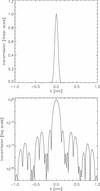 |
Fig. 1. Theoretical transmission profile of the narrow-band Lyot filter of Hinode/SOT NFI corresponding to observations at the Hα line core. The transmission profile is plotted in the linear scale (top) and the logarithmic scale (bottom). The logarithmic scale reveals the multiple transmission side lobes. |
To further process the synthetic intensities, we need to convert them to the observed units, that is, to digital counts (DC). To do so, we use the reference Hα profiles of David (1961) which are computed at various positions on the solar disk and are expressed in the units of erg s−1 cm−2 sr−1 Hz−1, as are the used synthetic intensities. In the present study, we computed the line core intensity of the reference Hα profile at the heliocentric angle of 78.5° as if observed through the Hinode/SOT NFI. The resulting value was then compared with a mean of observed values of Hα intensity obtained by Hinode/SOT NFI at the same disk position in the prominence observations discussed in the following section. We used the ratio of these two values as the conversion factor between units of erg s−1 cm−2 sr−1 Hz−1 and DC units.
To estimate the extent of the Hinode/SOT stray light and to asses the level of the noise in the observed data, we use observations of the solar north pole taken on May 3, 2010, at 15:00 UT (see Fig. 2) because they do not contain any structures of solar origin above the limb. From the highly saturated image in Fig. 2, it is clear that there are very weak signals extending more than 60″ above the limb. These signals, which gradually faint with altitude, are possibly caused by parasitic reflections within the satellite. To obtain the radial decrease of the measured signal above the solar limb, we averaged the central part of the image in Fig. 2 along the x-axis. The position of the solar limb was defined at a threshold of 100 DC to eliminate the influence of spicules. The resulting radial profile of the stray-light signal was added to the synthetic Hα intensity maps. We note that in Fig. 2, a small difference between the left and the right half of the image is apparent. This difference is caused by the fact that the Hinode/SOT detector consists of two individual CCDs.
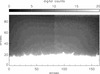 |
Fig. 2. Highly saturated image of the Hinode/SOT NFI observations of the solar north pole obtained on May 3, 2010, at 15:00 UT in the Hα line core. This image shows very weak signals extending more than 60″ above the limb. These signals were used to estimate the stray light and noise levels of the Hinode/SOT NFI. |
To estimate the noise level in the Hinode/SOT NFI data, we again used the observations shown in Fig. 2. From the original image (IM1), we subtracted the same, but this time spatially smoothed, image. The subtracted image (IM2) corresponds to the noise level in areas without any structures of solar origin. Such areas were identified using a threshold value of 20 DC in IM1. The histogram of values of IM2 in these areas was fitted by a double Gaussian function which was then used to generate random noise added to the synthetic Hα intensity maps.
4. Influence of Hinode/SOT NFI instrumental effects on synthetic Hα images
In this section, we analyze the influence of the instrumental effects of Hinode/SOT NFI on the visibility of the simulated prominence fine structures in synthetic Hα images. To do so, we processed the synthetic Hα intensity maps from GM and GDASH models (see Sect. 2) by taking into account all instrumental effects described in Sect. 3. Below, we compare the resulting SOT-like synthetic Hα images with the synthetic images obtained in the Hα line center. In addition, we compare the SOT-like synthetic images with selected prominences observed by Hinode/SOT NFI. However, we want to emphasize that this comparison is qualitative because the current 3D WPFS models do not aim to reproduce any specific observed prominence.
For the comparison with observations, we selected two prominences observed by Hinode/SOT NFI in the Hα line core. The first prominence was observed on Feb 14, 2012, at 10:51 crossing the NW limb at 28° N (x = 868″, y = 466″). This quiescent prominence is in the vicinity of an active region and may be connected to it. This type of quiescent prominence is represented by the GM model (see Gunár & Mackay 2015a, for more details). The second prominence was observed on Feb 23, 2012, at the SW limb (60° S; x = 511″, y = −844″) and represents a typical quiet-sun quiescent prominence.
In Fig. 3 we show a comparison between the synthetic SOT-like intensity maps of the GM model (top row) and the GDASH model (the second row), together with the duo of selected quiescent prominences. In the left column, we plot intensity maps in a linear scale and in the right column we plot the same maps in a logarithmic scale. Intensities in each column are plotted in an identical color scale. This allows us to relate the intensities in the synthetic and observed images. We note that this is the first qualitative comparison involving any of the WPFS models and prominence observations. The comparison shows that in the selected observed prominences, the maximum intensities are about half of the maximum intensities in the models. While comparable, such a difference can be explained by the fact that the models use mass-loading which is filling the maximum volume of the dipped prominence magnetic field with simulated prominence fine structures. This mass-loading can be, however, realistically scaled down by simply considering a lower percentage of magnetic dips to be filled Gunár & Mackay (2015a, see for more details). Another contributing factor to the difference between the level of the Hα intensities in the synthetic maps and in the observations could be the lack of dynamics in the current 3D WPFS models. All simulated fine structures in the models are static while fine structures in observed prominences are naturally dynamic. However, the movement of fine structures will generally result in lower observed maximum intensities compared to a static case. The reason for this is two-fold. First, the Doppler-shift effect causes a spectral line to shift with respect to the instrument response profile. Because the Hα line is an emission line without a self reversal, any shift between the line-center wavelength (where the specific intensity in Hα is the highest) and the instrument response profile will result in lower integrated intensities. The second reason is the fact that dynamic fine structures would tend to be spatially more spread, resulting in a generally smaller number of fine structures being crossed by a given LOS than in a static case. This would tend to produce lower intensities. While the comparison between the prominence models and observations presented here is encouraging, a quantitative analysis involving a large number of observed prominences will be needed to establish the right amount of mass-loading in the models.
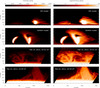 |
Fig. 3. Comparison between the synthetic SOT-like images provided by the 3D WPFS model of Gunár & Mackay (2015a, the GM model, top row), the 3D WPFS model of Gunár et al. (2018a, the GDASH model, second row,) and selected quiescent prominences observed by Hinode/SOT NFI on Feb 14 and Feb 23, 2012. In the left column, we plot the intensities in the linear scale and in the right column we plot the same intensities in the logarithmic scale. Intensities in each column are expressed in units of digital counts (DC) and plotted in an identical color scale. The field of view in all panels is identical and dimensions are expressed in arcsec. |
In addition to the difference in the intensities, we can use Fig. 3 to study the qualitative similarities and differences between the general structures (large and small) visible in the models and observations. While the large-scale prominence features appear rather similar in the models and in the observations, none of the models can reproduce the overall complexity of the observed prominences. Such an outcome is indeed expected because the current WPFS models are based on simplified photospheric magnetic flux distributions when compared to the complex photospheric flux carpet underlying actual prominences. Therefore, in the selected observed prominences we can see that in the linear scale, the large column-like features are similar to the brightest vertical parts of the simulated prominences, including the V-shaped parts visible in rows 2 and 3 of Fig. 3. Moreover, in the logarithmic scale, we can identify the prevalence of horizontally oriented fine structures in both models and observations, for example in the prominence observed on Feb 14, 2012 (the third row of Fig. 3). However, the distribution of these fine structures is less organized in the observations than in the models. In addition, the diffuse intensity region encompassing the entire prominence observed on Feb 14, 2012, is not present in the models.
From the comparison between the intensity maps displayed in the linear (left column of Fig. 3) and logarithmic scale (right column of Fig. 3), it is obvious that in the linear scale we can discern more structuring in the brightest parts of prominences while in the logarithmic scale we can study the faintest features. The top parts of prominences tend to consist of rather faint fine structures. In the models, this is due to the shallow depth of the magnetic dips at the apex of prominences. Therefore, the visualization using the logarithmic scale is important for a proper understanding of the prominence height.
The difference between the linear and logarithmic visualizations is more easily visible in Fig. 4. In this figure we use a detailed view of the GDASH model to compare the Hα line-center visualization employed in the current 3D WPFS models (see Heinzel et al. 2015, for more details) with the SOT-like Hα images which include all instrumental effects of the Hinode/SOT NFI (see Sect. 3). In the top row of Fig. 4, we show the Hα line-center intensity maps in the linear scale (left) and the logarithmic scale (right). In the bottom row, we use the same view but in the calibrated SOT-like synthetic images, again in the linear (left) and logarithmic (right) scales. It is clear that the finest prominence features appear less sharp in the SOT-like images than in the Hα line-center maps. However, all large- and small-scale structures characterizing this simulated prominence can be clearly discerned in both visualizations.
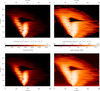 |
Fig. 4. Comparison between the Hα line-center visualization technique used in the current 3D WPFS models and the SOT-like Hα visualization that includes the Hinode/SOT NFI instrumental effects. In all panels, we show a detailed view of the GDASH model. In the top row, we display the synthetic images in Hα line-center and in the bottom row the synthetic SOT-like Hα images. In the left column, we plot intensities in the linear scale and in the right column in the logarithmic scale. All intensities are plotted in an identical color scale in units of erg s−1 cm−2 sr−1 Hz−1 (top row) and digital counts (DC, bottom row). Dimensions are expressed in arcsec. |
The added level of noise and stray light is apparent in the logarithmic scale, where indeed some of the faintest fine structures blend into the background. However, most of the fine structures, especially those at the top of the simulated prominence, can be easily identified in both visualizations. This comparison demonstrates that the Hα line-center visualization technique produces images which are very similar to the SOT-like synthetic Hα images. To confirm these findings, we use a scatter-plot comparing pixel-by-pixel intensities in the Hα line-center images and the SOT-like images. Both models (GM and GDASH) are combined in the resulting plot. Figure 5 thus demonstrates the combined role of all Hinode/SOT NFI instrumental effects that we take into account – PSF, integration over the transmission profile of NFI Lyot filter, stray light, and noise. The data-points in the scatter-plot do not significantly spread out from the red line that represents the Hα line-center intensity values converted into DC units using the correction factor described in Sect. 3. Any deviation of data-points from this line is caused by NFI instrumental effects. The effect of spatial PSF convolution is the most obvious as the brightest pixels in the simulation are smoothed and lie below the red line while the faintest signals are enhanced due to the smoothing with nearby brighter regions and the pixels are predominantly located above the red line. The overall small discrepancy between the Hα line-center and SOT-like intensities is highlighted by the green contour marking the peak of the probability density function. The contour encompasses an area containing 60% of all data-points. The small influence of NFI instrumental properties is also indicated by the linear fit (blue line) to all plotted data-points. The linear fit also does not deviate significantly from the red line.
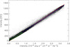 |
Fig. 5. Scatter-plot showing a pixel-by-pixel comparison between intensities in the Hα line-center images (x-axis) and the SOT-like images (y-axis). Data from both GM and GDASH models are combined and pixels with very weak signal are excluded. The red line represents the Hα line-center intensity values converted into DC units. The blue line indicates a linear fit to the plotted data-points. The green contour marks the peak of the probability density function of the displayed data-points and encompasses an area containing 60% of all data-points. |
5. Conclusions
Models that simulate prominences with their numerous fine structures distributed within the prominence magnetic field are becoming ever more complex. This creates a need for reliable visualization techniques that can mimic the radiative transfer processes within the prominence plasma. The fast approximate Hα visualization method of Heinzel et al. (2015) is one such technique. Thanks to such models and visualization techniques, we can now study in detail the links between the configuration of prominence magnetic field, the distribution and the properties of prominence fine structure plasma, and the radiative processes within the prominence plasma. The radiation emergent from this plasma conveys to us all the information we gain by observing prominences (see e.g., Gunár & Mackay 2015b, 2016; Gunár et al. 2016, 2018b). However, to properly understand both large- and small-scale morphological features and dynamics of prominences, we need to be confident that the techniques we use for the visualization of simulated prominences provide the same kind of information as observations. Therefore, it is important to understand how the visibility of simulated prominences would be affected by the properties of instruments used for observations. For example, we need to know which prominence features would still be visible and which would be indistinguishable from the background level of noise and stray light. In the present work, we study for the first time the influence of properties of an observing instrument on the visibility of modeled prominence structures in synthetic images. To do so, we focus here on Hinode/SOT NFI and produce SOT-like synthetic Hα images which incorporate integration of the synthetic Hα spectra over the narrowband transmission filter, together with the effects of instrument PSF, stray light, and noise. Only such processed synthetic Hα images can be directly compared with observations.
In this study, we selected a pair of Hinode/SOT NFI observations of quiescent prominences which we compare with the SOT-like synthetic Hα images of the GM (Gunár & Mackay 2015a) and GDASH (Gunár et al. 2018a) models. This comparison (see Fig. 3) shows that the 3D WPFS models can reproduce large-scale prominence features rather well. However, the distribution of the prominence fine structures is significantly more diffuse in the observations than in the models. This could be a consequence of the photospheric flux distributions used in the models, which are more simple than the photospheric flux carpet underlying the actual prominences. Another explanation could be the lack of dynamics in the models, which would cause the same number of fine structures to appear more scattered in the plane of the sky. The models also cannot reproduce the diffuse intensity areas surrounding the observed prominences. Such diffuse intensity, which is also present in the openings within the observed prominences, does not appear in the SOT-like synthetic Hα images of the 3D models. This diffuse intensity could be partially caused by an additional stray-light contribution due to the presence of a relatively bright prominence in the FOV. However, such a diffuse intensity could also be an indication of a low-density or higher-temperature plasma surrounding the dense and cool parts of prominences – a so-called halo prominence-corona transition region (see e.g., the discussion in Gunár et al. 2014).
Apart from the investigation of the prominence morphology, the SOT-like synthetic Hα images allow us to directly compare the calibrated intensities between the models and observations. We found here that the maximum intensities reached in the models are about twice as high as those present in the observations. This suggests that the mass-loading assumed in the present 3D WPFS models might be too large. The amount of the prominence plasma in the models can easily be scaled down however; a future detailed analysis involving a large number of Hinode/SOT prominence observations will be needed to address this issue.
Another result of the work presented here is the comparison (see Fig. 4) between the SOT-like synthetic Hα images and the synthetic images produced by the 3D WPFS models of Gunár & Mackay (2015a) and Gunár et al. (2018a), which use only the specific intensity in the Hα line center for the visualization of the simulated prominences. Such a visualization technique, while being computationally efficient, is only an approximation of the processes which lead to actual observations. To demonstrate that the Hα line-center visualization technique produces reliable synthetic images, we compare images produced using this latter method with the SOT-like synthetic Hα images. This comparison shows that both large- and small-scale features are very similar in both visualizations. Moreover, we also show that the same very faint prominence fine structures can be discerned in both sets of synthetic images, especially when the logarithmic scale is used. This comparison therefore confirms that the computationally efficient Hα line-center visualization technique can be reliably used for the purpose of visualization of complex 3D prominence models. However, to quantitatively compare any prominence models with actual observed prominences, it is necessary to include all instrumental effects and to integrate the synthetic spectra over the transmission profile of a used instrument. It is also important to note that our conclusions are valid for the seeing-free space-borne observations, such as those of Hinode/SOT. Observations obtained by ground-based instruments are naturally influenced by the immediate atmospheric conditions which may further affect the visibility of the prominence fine structures. Therefore, a careful analysis of the adequacy of the Hα line-center visualization technique for ground-based observations is necessary.
Acknowledgments
S.G. acknowledges support from the grant No. 19-16890S of the Czech Science Foundation (GA ČR). S.G. and J.J. thank for the support from project RVO:67985815 of the Astronomical Institute of the Czech Academy of Sciences.
References
- Amari, T., Canou, A., & Aly, J.-J. 2014, Nature, 514, 465 [NASA ADS] [CrossRef] [Google Scholar]
- Aulanier, G., & Démoulin, P. 1998, A&A, 329, 1125 [Google Scholar]
- David, K.-H. 1961, ZAp, 53, 37 [Google Scholar]
- Démoulin, P., & Aulanier, G. 2010, ApJ, 718, 1388 [NASA ADS] [CrossRef] [Google Scholar]
- Gibson, S. E. 2018, Liv. Rev. Solar Phys., 15, 7 [NASA ADS] [CrossRef] [Google Scholar]
- Gunár, S. 2014, in IAU Symposium, eds. B. Schmieder, J. M. Malherbe, & S. T. Wu, 300, 59 [NASA ADS] [Google Scholar]
- Gunár, S., & Mackay, D. H. 2015a, ApJ, 803, 64 [NASA ADS] [CrossRef] [Google Scholar]
- Gunár, S., & Mackay, D. H. 2015b, ApJ, 812, 93 [NASA ADS] [CrossRef] [Google Scholar]
- Gunár, S., & Mackay, D. H. 2016, A&A, 592, A60 [NASA ADS] [CrossRef] [EDP Sciences] [Google Scholar]
- Gunár, S., Heinzel, P., Anzer, U., & Schmieder, B. 2008, A&A, 490, 307 [NASA ADS] [CrossRef] [EDP Sciences] [Google Scholar]
- Gunár, S., Schwartz, P., Schmieder, B., Heinzel, P., & Anzer, U. 2010, A&A, 514, A43 [NASA ADS] [CrossRef] [EDP Sciences] [Google Scholar]
- Gunár, S., Mein, P., Schmieder, B., Heinzel, P., & Mein, N. 2012, A&A, 543, A93 [NASA ADS] [CrossRef] [EDP Sciences] [Google Scholar]
- Gunár, S., Mackay, D. H., Anzer, U., & Heinzel, P. 2013, A&A, 551, A3 [NASA ADS] [CrossRef] [EDP Sciences] [Google Scholar]
- Gunár, S., Schwartz, P., Dudík, J., et al. 2014, A&A, 567, A123 [NASA ADS] [CrossRef] [EDP Sciences] [Google Scholar]
- Gunár, S., Heinzel, P., Mackay, D. H., & Anzer, U. 2016, ApJ, 833, 141 [NASA ADS] [CrossRef] [Google Scholar]
- Gunár, S., Dudík, J., Aulanier, G., Schmieder, B., & Heinzel, P. 2018a, ApJ, 867, 115 [NASA ADS] [CrossRef] [Google Scholar]
- Gunár, S., Heinzel, P., Anzer, U., & Mackay, D. H. 2018b, ApJ, 853, 21 [NASA ADS] [CrossRef] [Google Scholar]
- Heinzel, P., & Anzer, U. 2001, A&A, 375, 1082 [NASA ADS] [CrossRef] [EDP Sciences] [Google Scholar]
- Heinzel, P., Gunár, S., & Anzer, U. 2015, A&A, 579, A16 [NASA ADS] [CrossRef] [EDP Sciences] [Google Scholar]
- Jenkins, J. M., Hopwood, M., Démoulin, P., et al. 2019, ApJ, 873, 49 [NASA ADS] [CrossRef] [Google Scholar]
- Kliem, B., & Török, T. 2006, Phys. Rev. Lett., 96, 255002 [NASA ADS] [CrossRef] [PubMed] [Google Scholar]
- Kosugi, T., Matsuzaki, K., Sakao, T., et al. 2007, Sol. Phys., 243, 3 [NASA ADS] [CrossRef] [Google Scholar]
- Labrosse, N., Heinzel, P., Vial, J., et al. 2010, Space Sci. Rev., 151, 243 [Google Scholar]
- Mackay, D. H., & van Ballegooijen, A. A. 2009, Sol. Phys., 260, 321 [NASA ADS] [CrossRef] [Google Scholar]
- Mackay, D. H., Karpen, J. T., Ballester, J. L., Schmieder, B., & Aulanier, G. 2010, Space Sci. Rev., 151, 333 [NASA ADS] [CrossRef] [Google Scholar]
- Parenti, S. 2014, Liv. Rev. Solar Phys., 11, 1 [Google Scholar]
- Schmieder, B., Malherbe, J. M., & Wu, S. T. 2014, in Nature of Prominences and their role in Space Weather, IAU Symp., 300 [Google Scholar]
- Tsuneta, S., Ichimoto, K., Katsukawa, Y., et al. 2008, Sol. Phys., 249, 167 [NASA ADS] [CrossRef] [Google Scholar]
- van Noort, M. 2012, A&A, 548, A5 [NASA ADS] [CrossRef] [EDP Sciences] [Google Scholar]
- Vial, J. C., & Engvold, O. 2015, in Solar Prominences, Astrophys. Space Sci. Libr., 415 [Google Scholar]
- Zuccarello, F. P., Aulanier, G., & Gilchrist, S. A. 2016, ApJ, 821, L23 [NASA ADS] [CrossRef] [Google Scholar]
All Figures
|
Fig. 1. Theoretical transmission profile of the narrow-band Lyot filter of Hinode/SOT NFI corresponding to observations at the Hα line core. The transmission profile is plotted in the linear scale (top) and the logarithmic scale (bottom). The logarithmic scale reveals the multiple transmission side lobes. |
| In the text | |
|
Fig. 2. Highly saturated image of the Hinode/SOT NFI observations of the solar north pole obtained on May 3, 2010, at 15:00 UT in the Hα line core. This image shows very weak signals extending more than 60″ above the limb. These signals were used to estimate the stray light and noise levels of the Hinode/SOT NFI. |
| In the text | |
|
Fig. 3. Comparison between the synthetic SOT-like images provided by the 3D WPFS model of Gunár & Mackay (2015a, the GM model, top row), the 3D WPFS model of Gunár et al. (2018a, the GDASH model, second row,) and selected quiescent prominences observed by Hinode/SOT NFI on Feb 14 and Feb 23, 2012. In the left column, we plot the intensities in the linear scale and in the right column we plot the same intensities in the logarithmic scale. Intensities in each column are expressed in units of digital counts (DC) and plotted in an identical color scale. The field of view in all panels is identical and dimensions are expressed in arcsec. |
| In the text | |
|
Fig. 4. Comparison between the Hα line-center visualization technique used in the current 3D WPFS models and the SOT-like Hα visualization that includes the Hinode/SOT NFI instrumental effects. In all panels, we show a detailed view of the GDASH model. In the top row, we display the synthetic images in Hα line-center and in the bottom row the synthetic SOT-like Hα images. In the left column, we plot intensities in the linear scale and in the right column in the logarithmic scale. All intensities are plotted in an identical color scale in units of erg s−1 cm−2 sr−1 Hz−1 (top row) and digital counts (DC, bottom row). Dimensions are expressed in arcsec. |
| In the text | |
|
Fig. 5. Scatter-plot showing a pixel-by-pixel comparison between intensities in the Hα line-center images (x-axis) and the SOT-like images (y-axis). Data from both GM and GDASH models are combined and pixels with very weak signal are excluded. The red line represents the Hα line-center intensity values converted into DC units. The blue line indicates a linear fit to the plotted data-points. The green contour marks the peak of the probability density function of the displayed data-points and encompasses an area containing 60% of all data-points. |
| In the text | |
Current usage metrics show cumulative count of Article Views (full-text article views including HTML views, PDF and ePub downloads, according to the available data) and Abstracts Views on Vision4Press platform.
Data correspond to usage on the plateform after 2015. The current usage metrics is available 48-96 hours after online publication and is updated daily on week days.
Initial download of the metrics may take a while.