| Issue |
A&A
Volume 629, September 2019
|
|
|---|---|---|
| Article Number | A52 | |
| Number of page(s) | 12 | |
| Section | Galactic structure, stellar clusters and populations | |
| DOI | https://doi.org/10.1051/0004-6361/201936056 | |
| Published online | 03 September 2019 | |
Anatomy of a buckling galactic bar
Nicolaus Copernicus Astronomical Center, Polish Academy of Sciences, Bartycka 18, 00-716 Warsaw, Poland
e-mail: lokas@camk.edu.pl
Received:
10
June
2019
Accepted:
24
July
2019
Using N-body simulations we study the buckling instability in a galactic bar forming in a Milky Way-like galaxy. The galaxy is initially composed of an axisymmetric, exponential stellar disk embedded in a spherical dark matter halo. The parameters of the model are chosen so that the galaxy is mildly unstable to bar formation and the evolution is followed for 10 Gyr. A strong bar forms slowly over the first few gigayears and buckles after 4.5 Gyr from the start of the simulation becoming much weaker and developing a pronounced boxy/peanut shape. We measure the properties of the bar at the time of buckling in terms of the mean acceleration, velocity, and distortion in the vertical direction. The maps of these quantities in face-on projections reveal characteristic quadrupole patterns which wind up over a short timescale. We also detect a secondary buckling event lasting much longer and occurring only in the outer part of the bar. We then study the orbital structure of the bar in periods before and after the first buckling. We find that most of the buckling orbits originate from x1 orbits supporting the bar. During buckling the ratio of the vertical to horizontal frequency of the stellar orbits decreases dramatically and after buckling the orbits obey a very tight relation between the vertical and circular frequency: 3ν = 4Ω. We propose that buckling is initiated by the vertical resonance of the x1 orbits creating the initial distortion of the bar that later evolves as kinematic bending waves.
Key words: galaxies: evolution / galaxies: fundamental parameters / galaxies: kinematics and dynamics / galaxies: spiral / galaxies: structure
© ESO 2019
1. Introduction
We have known for a few decades now that galactic disks are inherently unstable and form bars easily (Miller et al. 1970; Ostriker & Peebles 1973). Although the presence of a dark matter halo modifies the process (Athanassoula 2003), this instability has been accepted as the main channel of bar formation in galaxies (for a review see Athanassoula 2013). Another possible scenario for the origin of bars involves tidal interactions of galactic disks with perturbers of different sizes (Noguchi 1996; Miwa & Noguchi 1998; Łokas et al. 2014, 2016; Gajda et al. 2017, 2018; Łokas 2018; Peschken & Łokas 2019). Such tidally induced bars result from sufficiently strong tidal deformations and are in all aspects similar to those formed in isolation, although perhaps have smaller pattern speeds.
Independently of their origin, strong bars tend to undergo an event of buckling instability during their evolution (Combes & Sanders 1981; Pfenniger & Friedli 1991; Raha et al. 1991; Athanassoula 2016; Smirnov & Sotnikova 2019; Łokas 2019). The phenomenon has been studied using N-body simulations and shown to involve significant distortions of the bar out of the disk plane that thicken and weaken the bar, but do not destroy it; although the presence of gas has been argued to suppress buckling (Debattista et al. 2006; Berentzen et al. 2007; Villa-Vargas et al. 2010). The instability may occur more than once in the lifetime of a bar, with the second episode usually lasting longer and happening in the outer parts of the bar (Martinez-Valpuesta et al. 2006). The event leaves behind a distinct boxy/peanut shape in the inner part of the bar similar to bulges of some late-type galaxies (Debattista et al. 2004; Athanassoula 2005; Bureau et al. 2006; Yoshino & Yamauchi 2015; Erwin & Debattista 2016, 2017; Li et al. 2017; Savchenko et al. 2017). Buckling probably also took place in the bar of the Milky Way, as evidenced by the boxy/peanut structure (Weiland et al. 1994; Ciambur et al. 2017), possibly leaving its traces in the presently observable phase-space (Khoperskov et al. 2019).
The nature of buckling instability remains unclear. Combes et al. (1990) and Pfenniger & Friedli (1991) were the first to propose that the instability results from trapping x1 orbits of the bar at vertical resonances. However, such resonances are expected to apply only to banana-like orbits that have been shown to contribute only a little to the final boxy/peanut shape (Patsis et al. 2002; Portail et al. 2015; Valluri et al. 2016; Abbott et al. 2017; Patsis & Harsoula 2018). An alternative hypothesis for the origin of the instability involves the ratio of the vertical to horizontal velocity dispersion of the stars in the bar and relates it to the fire-hose instability (Toomre 1966; Raha et al. 1991; Merritt & Hernquist 1991; Merritt & Sellwood 1994). In this picture, the instability is supposed to be triggered by a sufficiently low dispersion ratio of the order of 0.3, characteristic of strong bars.
In Łokas (2019) we used simulations of tidally induced galactic bars from Łokas (2018) to study buckling instability. Such configurations have the advantage that the same initial galaxy model can be used to create bars of different strength by different tidal forcings. We demonstrated that for such bars there is no direct relation between the ratio of the vertical to radial velocity dispersion and the susceptibility of the bar to buckling, suggesting that buckling is due to vertical orbital resonances rather than the fire-hose instability. This conclusion was supported by an approximate calculation of the vertical and horizontal resonances, which were shown to coincide during buckling. Although tidal interactions may be an important or even dominant scenario for the formation of galactic bars (Peschken & Łokas 2019), the difficulty in using tidally induced bars is that during tidal interactions in addition to bars strong spiral arms are formed which later wind up and may disturb the orbital structure.
In this work we therefore revisit the issue of buckling instability using a simulation of an isolated galaxy initially composed of an axisymmetric exponential disk and a dark matter halo. The bar develops in the disk over a few gigayears of evolution and then buckles. In addition to different measures of distortion introduced in Łokas (2019) we characterize buckling by studying the orbital structure of the bar before and after buckling. For this purpose we apply the spectral analysis of stellar orbits as pioneered by Binney & Spergel (1982). This approach has been developed over the years and successfully used to study the orbital structure of different potentials, including galactic bars (Miralda-Escudé & Schwarzschild 1989; Papaphilippou & Laskar 1996; Carpintero & Aguilar 1998; Valluri & Merritt 1998; Merritt & Valluri 1999; Voglis et al. 2007; Ceverino & Klypin 2007; Deibel et al. 2011; Valluri et al. 2010, 2012, 2016; Portail et al. 2015), although most of these studies relied on test particle orbits evolved in static external potentials. Gajda et al. (2016) demonstrated that the orbital structure can be reliably measured also “in vivo”, that is in a live bar evolving in an N-body simulation, even in configurations that are not stationary by construction, for example in dwarf galaxies orbiting the Milky Way.
The paper is organized as follows. In Sect. 2 we provide the details of the simulation used in this study and characterize the evolution of the bar formed in the galaxy. Section 3 presents the description of the buckling instability in terms of the mean acceleration, streaming velocity, and distortion of the stars out of the disk plane in the vertical direction, measured both radially and in the face-on projection. The orbital structure of the bar before and after buckling is studied in Sect. 4 and the discussion follows in Sect. 5.
2. The simulated bar
For the purpose of this study we ran an N-body simulation of a two-component galaxy with properties similar to the Milky Way. The exact parameters were chosen, after a few trial simulations, so that the galaxy forms the bar relatively slowly, with it becoming strong enough to buckle after a few gigayears of evolution.
The galaxy initially contained two components: a spherical dark matter halo and an exponential disk. The structural parameters of the galaxy were the following: its dark matter halo had an Navarro-Frenk-White (Navarro et al. 1997) profile with a virial mass MH = 1012 M⊙ and concentration c = 25 while the exponential disk had a mass MD = 4.5 × 10¹⁰ M⊙, scale-length RD = 3 kpc, and thickness zD = 0.42 kpc. The central value of the radial velocity dispersion was σR, 0 = 120 km s−1. The minimum value of the Toomre parameter for this model at 2.5RD was Q = 1.73. We note that with this choice of parameters the contribution to the rotation curve from the disk and the halo in the inner parts is very similar.
The N-body realization of the galaxy was initialized using the procedures described in Widrow & Dubinski (2005) and Widrow et al. (2008) with each component containing 106 particles. The evolution of the galaxy was followed for 10 Gyr with the GIZMO code (Hopkins 2015), an extension of the widely used GADGET-2 (Springel et al. 2001; Springel 2005), saving outputs every 0.05 Gyr. The adopted softening scales were ϵD = 0.03 kpc and ϵH = 0.06 kpc for the disk and halo of the galaxy, respectively, within the ranges recommended by Hopkins et al. (2018).
The evolution of the global shape of the stellar component of the galaxy is illustrated in Fig. 1. For the purpose of these and the following measurements the stars within 2RD were used to determine the orientation and lengths of the principal axes of the stellar distribution in each output and the stellar component was rotated to align the longest axis with x, the intermediate one with y, and the shortest one with z coordinate of a Cartesian coordinate system that is used throughout the paper. The upper panel of Fig. 1 shows the evolution of the axis ratios b/a and c/a where a is the longest, b the intermediate, and c the shortest axis. In the lower panel we characterize the shape with a combination of axis ratios in the form of the triaxiality parameter T = [1 − (b/a)2]/[1 − (c/a)2].
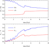 |
Fig. 1. Evolution of the shape of the stellar component in time. Upper panel: evolution of the axis ratios b/a (intermediate to longest axis) and c/a (shortest to longest axis). Lower panel: triaxiality parameter T = [1 − (b/a)2]/[1 − (c/a)2] and the bar mode A2. Measurements were made for stars within the radius of 2Rd. |
The lower panel of Fig. 1 also shows the strength of the bar measured as the m = 2 mode of the Fourier decomposition of the surface distribution of stars within 2RD projected along the short axis: Am(R) = |Σjexp(imθj)|/Ns. Here θj is the azimuthal angle of the jth star and the sum is up to the total number of Ns stars. The radius R is the standard radius in cylindrical coordinates in the plane of the disk, R = (x2 + y2)1/2.
The axis ratio b/a decreasing from unity and the growth of the triaxiality parameter T and the bar mode A2 from zero, characteristic of disks, to much larger values signify the formation of a bar in the stellar component of the galaxy. The bar grows until t = 4.3 Gyr, when a sudden drop occurs in both T and A2 while both b/a and c/a sharply increase. This time marks the occurrence of the buckling event which weakens and thickens the bar.
The bar may be characterized in more detail by calculating the profiles of the bar mode as a function of the cylindrical radius, A2(R). A few examples of such profiles at different times are shown in Fig. 2. They all display a characteristic shape, with a strong growth from zero at small radii, followed by a maximum, and then a decrease. The radius where A2(R) drops down to half the maximum value is usually adopted as an estimate of the bar length. Before the buckling event at t = 4.3 Gyr, the bar is already quite strong with the maximum of A2(R) = 0.56 and the length of the order of 7 kpc. Immediately after buckling, at t = 5 Gyr, the profile is significantly lower with a maximum at A2(R) = 0.45 and the length also decreased by about 1 kpc. Later on, the bar grows both in strength and length until t = 10 Gyr.
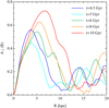 |
Fig. 2. Profiles of the bar mode A2(R) at different times. |
The profiles of the bar mode A2(R) for all outputs can be combined and color-coded to describe the whole history of the bar evolution in time, as shown in Fig. 3. From this plot it can be seen that the bar starts to form around t = 1.5 Gyr in the sense that it crosses the threshold of 0.1 in A2(R) for the first time. The buckling around t = 4.5 Gyr is also visible as a drop of the maximum of A2(R) from above to below 0.5. At later times the growth of the bar seems undisturbed, especially after t = 8 Gyr.
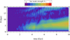 |
Fig. 3. Evolution of the profiles of the bar mode A2(R) over time. |
3. Description of the buckling instability
Buckling also manifests itself in the evolution of the velocity dispersions of the stars along the bar and perpendicular to it, which gave rise to its association with the fire-hose instability. In the upper panel of Fig. 4 we plot the evolution of the velocity dispersion along the cylindrical radius σR and along the vertical direction σz while the lower panel shows the ratio σz/σR as a function of time. Here again the measurements were done using only the stars within 2RD. We can see that the evolution of σR follows that of the bar mode A2 in the lower panel of Fig. 1 and is due to the fact that as the bar becomes stronger, more stars are on radial orbits or the orbits are more radial. On the other hand, σz grows only weakly, similarly to the thickness of the bar. The situation changes abruptly at t = 4.3 Gyr when σR suddenly drops down while σz grows. The event is even more emphasized in the ratio σz/σR shown in the lower panel of Fig. 4. It has been suggested in the past that the low value of σz/σR immediately before buckling is the reason for its occurrence because it leads to a kind of fire-hose instability which moves the stars out of the disk plane and then leaves the bar thickened. We note, however, that the minimum value of σz/σR immediately before buckling is much higher than the canonical value of 0.3 derived theoretically for some idealized configurations and thus speaks against this interpretation. Therefore, it is possible that the departures of the stars out of the disk plane are due to resonances between the radial and vertical motions.
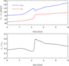 |
Fig. 4. Evolution of velocity dispersions of the stellar component over time. Upper panel: velocity dispersions along the cylindrical radius σR and along the vertical direction σz while lower panel: ratio σz/σR. Measurements were made for stars within the radius of 2RD. |
While the dispersions only measure the random motion of the stars in a given direction, it is much more instructive to study the acceleration and the streaming velocity of the stars as well as their distortion along the vertical direction. One way to do this is to calculate these quantities in shells along the cylindrical radius. The results of such measurements in terms of the profiles of the mean acceleration ⟨az⟩, mean velocity ⟨υz⟩, and the mean distortion of the positions of the stars along the vertical axis ⟨z⟩ as a function of time are shown color-coded in Fig. 5 in the three panels, respectively. The time range covered in these plots was restricted to between t = 4 and t = 8 Gyr when the signal is nonzero. We immediately see a strong buckling event with a maximum at t = 4.5 Gyr starting with a smile-like distortion of the bar which very soon after, around t = 4.6 Gyr, changes into a frown-like one (with respect to the direction of the angular momentum vector of the galaxy). After this the distortion propagates outward and becomes very weak already at t = 5 Gyr. We note that, as expected, the direction of the acceleration is opposite to the distortion and the signal in the acceleration starts to be visible at earlier times.
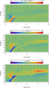 |
Fig. 5. Evolution of the profiles of the mean acceleration (upper panel), velocity (middle panel), and distortion of the positions of the stars (lower panel) along the vertical axis z. Positive quantities point along the angular momentum vector of the disk. |
Interestingly, later on, between t = 6.5 and t = 8 Gyr, a second buckling event takes place. This happens only at larger radii, R > 5 kpc, lasts much longer, and involves only one kind of distortion (downward then upward with radius), without a clear reversal that was present in the earlier episode of buckling. While no obvious signal of this buckling is seen in the evolution of the bar mode in Fig. 3, a hint of its presence can be seen in the evolution of the axis ratio c/a in the upper panel of Fig. 1, which increases around this time; albeit very slightly because the measurements there were done within 2RD = 6 kpc. We note that there is even a kind of continuity between the first and second buckling events as the weak distortion is present all the time between t = 5 and t = 6.5 Gyr. In this sense the first buckling event may be considered as a seed for the second one. Some examples of the edge-on view of the galaxy at different times during buckling are shown in Fig. 6.
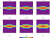 |
Fig. 6. Surface density distributions of the stellar component viewed edge-on before the first buckling (t = 4 Gyr), at the time of first buckling (t = 4.5, 4.65 and 5 Gyr), at the time of second buckling (t = 7.1 Gyr), and at the end of evolution (t = 10 Gyr). The surface density was normalized to the central maximum value in each case and the contours are equally spaced in logΣ with ΔlogΣ = 0.05. |
Even more insight into the structure of the bar during buckling can be obtained by plotting the maps of the mean vertical acceleration, velocity, and distortion in the face-on view. A few examples of such maps are shown in Figs. 7 and 8 for the same outputs as the corresponding surface density plots in the edge-on view in Fig. 6. In all plots the stellar component has been rotated so that the bar is aligned with the x axis, while its shortest axis (and the rotation axis of the disk) is along z and the disk is rotating counterclockwise.
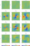 |
Fig. 7. Face-on maps of the mean acceleration (left column), mean velocity (middle column), and mean distortion of the positions of the stars (right column) along the vertical direction at the time of the first buckling. The four rows of panels show the results for times t = 4, 4.5, 4.65, and 5 Gyr. |
In the first row of panels in Fig. 7, corresponding to t = 4 Gyr, no clear signal in the acceleration, velocity, or distortion is visible yet, in agreement with Fig. 5. In the second row, at t = 4.5, a very strong signal is seen. We note that the regions of downward acceleration (in blue) and upward velocity and distortion (in red) are not located exactly along the bar (which is aligned with the x coordinate) and the regions of upward acceleration (in red) and downward velocity and distortion (in blue) are not exactly perpendicular to it. At the same time, the patterns in distortion and velocity are rotated with respect to each other by about 45 deg so that the regions of extreme distortion are aligned with the zero-velocity curves and vice versa, while the maxima of acceleration coincide with the maxima of distortion but have an opposite sign, as expected for an oscillatory motion in the vertical direction.
This growing pattern in acceleration, velocity, and distortion preserves its orientation with respect to the bar for about 0.2 Gyr, that is between t = 4.4 and t = 4.6. After this short period it starts to wind up, as shown in the third row of plots in Fig. 7. Later, at t = 5 Gyr (lower row of panels in Fig. 7), a weak pattern remains only in the outer parts of the bar (R > 5 kpc) while within the inner range of radii (R < 5 kpc) a clear boxy/peanut shape is formed (see Fig. 6).
Figure 8 illustrates the second buckling event that occurs in the outer parts of the bar (R > 5 kpc) between t = 6.5 and t = 8 Gyr. The upper set of panels shows the acceleration, velocity, and distortion maps at t = 7.1 Gyr when the buckling signal is strongest. A similar pattern in ⟨az⟩, ⟨υz⟩, and ⟨z⟩ is discernible, but only in the outskirts of the bar, while its inner part remains undisturbed. The origin of these distortions can be seen in the corresponding panel of Fig. 6 showing the surface density distribution of the stars. Clearly, there is a frown-like distortion dominating around R = 6 kpc and a smile-like one around R = 8 kpc. Later on, the pattern in all quantities dissipates leaving behind at the end of evolution (t = 10 Gyr) a much bigger boxy/peanut shape (see the lower right panel of Fig. 6).
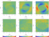 |
Fig. 8. Same as Fig. 7 but at the time of second buckling (upper row) and at the end of evolution (lower row). |
4. The orbital structure of the buckling bar
To obtain a deeper understanding of the buckling instability it seems indispensable to resort to the study of the orbital structure of the buckling bar. In this section we restrict the analysis of the orbits to the first, stronger buckling episode. For this purpose we reran the simulation in the 2 Gyr period between t = 3.5 and t = 5.5 Gyr saving 2001 outputs, that is, every 0.001 Gyr. This time resolution is sufficient to measure the properties of orbits for a majority of stars building up the bar. We also determined the orientation of the bar in each simulation output and transformed the orbits to the reference frame of the bar. We thus study the orbits in the Cartesian reference frame with x, y, and z aligned with the major, intermediate, and minor axes of the bar. The advantages of this approach in comparison to using the traditional cylindrical coordinates have been discussed in detail by Valluri et al. (2016) and Gajda et al. (2016).
A visual inspection of a few hundred orbits revealed that an abrupt change in their properties takes place around t = 4.5 Gyr, as suggested by the results of the previous section. We therefore divided this 2 Gyr period into three parts which we refer to as “before buckling”, “during buckling”, and “after buckling”. The first period of 0.7 Gyr falls between 3.5 and 4.2 Gyr, the second one lasting 0.6 Gyr is between 4.2 and 4.8 Gyr (and is therefore centered on the 4.5 Gyr time when the transition takes place) and the third one again lasting 0.7 Gyr is between 4.8 and 5.5 Gyr. It is certainly possible to measure the properties of the orbits when they are stable and therefore we take measurements only in the two periods of 0.7 Gyr before and after buckling.
Figure 9 shows an example of a stellar orbit that experiences buckling. Clearly the shape of the orbit is very different at the beginning; in particular its motion in the z direction (perpendicular to the bar) is confined to a very narrow range (left panels). During buckling the shape of the orbit experiences an abrupt change (middle panels) so that after buckling (right panels) the orbit covers a much larger range of z values. The oscillatory motion of the star in the directions perpendicular and parallel to the bar is shown in Fig. 10. Clearly, both the amplitude and the frequency of the motion change in each of the x and z directions.
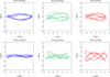 |
Fig. 9. Example of a buckling orbit. The orbit is plotted in different colors in three time periods: before, during, and after buckling (from the left to the right panel) and in two projections: in the face-on and edge-on view (the top and bottom row, respectively). After buckling the star follows a regular, periodic, pretzel-like orbit with frequency ratio fz, after/fx, after = 7/4, that is it completes four oscillations in x for every seven oscillations in z. |
We use time series such as the ones shown in Fig. 10 to calculate the frequencies of the orbits in the Cartesian coordinates x, y, and z using discrete Fourier transform. The calculations were done for the 0.7 Gyr time-periods before and after buckling that include 700 data points each. This time range needs to be long enough for the orbits to complete at least a few oscillations. On the other hand, we recall that the measurements of orbital properties here are done “in vivo”, that is in the live evolving bar, and therefore the time period considered should be as short as possible so that the bar properties can be approximated as constant. In order to obtain sufficiently accurate estimates of frequency we restrict the analysis to orbits with periods larger than 0.25 Gyr. For each orbit we also estimate the amplitude (or apocenter) in the three coordinates and require that the position of the star crosses the zero value (in the reference frame of the bar) at least once. These conditions eliminate the large nearly circular orbits that do not contribute to the bar. Such weak restrictions allow us to measure the properties of 475512 out of the total number of 106 stars.
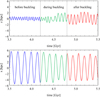 |
Fig. 10. Evolution of the position of the star along the minor and major axes of the bar for the orbit shown in Fig. 9. The time range of interest was divided into three parts: before, during, and after buckling, indicated with different colors. |
Since we are interested in the orbits that contribute to the buckling of the bar we further restrict the analysis to orbits that actually support the bar, that is: their x amplitude, ax, is within 7 kpc (the length of the bar) and their amplitude in the y direction, ay, is smaller than 0.7 of the x amplitude: ay < 0.7ax. We require that these conditions are fulfilled both before and after buckling. This way we eliminate for example x2 and x4 orbits that do not support the bar, as well as long-axis tubes in the center. In addition, we require that the orbits actually buckle, and therefore we take only those orbits that have larger amplitudes in z after buckling than before buckling: az, after > az, before. These restrictions leave us with a sample of 199601 orbits whose properties we study further.
A common way to characterize the orbital structure of a bar is to study the distribution of the frequency ratios. In Fig. 11 we show histograms of frequency ratios fy/fx and fz/fx before and after buckling. In the case of fy/fx most of the orbits contribute to the strong peak at fy/fx = 1 characteristic for x1 orbits, both before and after buckling. There is also an additional small contribution from other, box orbits with initial frequencies in the range 1.7−2.0. These orbits shift to values close to 3/2 after buckling although some of the x1 orbits also contribute to this new peak, since this range is more populated than the 1.7−2.0 range before buckling.
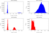 |
Fig. 11. Histograms of frequency ratios fy/fx (left column) and fz/fx (right column) before (upper row, blue) and after (lower row, red) buckling. |
A much more interesting evolution occurs in the ratio fz/fx. Before buckling, the orbits occupy a wide range of values between 1.8 and 4. After buckling they move to a much narrower range of much smaller values: 1.4−2.1. The reason for this can be partially understood by looking at the evolution of fz and fx separately, which is shown in Fig. 12. We can see that while the frequencies in the vertical direction, fz, typically decrease during buckling, those along the bar, fx, increase. The effect of this is obviously to strongly decrease the ratio fz/fx. Another way to look at this change is via a 2D histogram of the ratio fz/fx before and after buckling shown in Fig. 13. This plot can be helpful in mapping between fz, before/fx, before and fz, after/fx, after. The right-hand histograms of Fig. 11 can be viewed as projections of the 2D histogram in Fig. 13 in the vertical and horizontal directions.
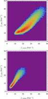 |
Fig. 12. Distribution of the stars in the plane of the frequency of the orbit along a given direction after buckling vs. the same frequency before buckling. Upper panel: results for the motion along z and lower panel: for the motion along x. The color coding in these 2D histograms and the following figures is such that the red corresponds to maximum occupation and violet to empty cells. |
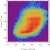 |
Fig. 13. Distribution of stars in the plane of frequency ratios fz, before/fx, before and fz, after/fx, after. |
Let us see how the orbits evolve in terms of frequency using the particular example of the orbit shown in Fig. 9. Before buckling, the frequency ratios for this orbit are fy, before/fx, before = 1 and fz, before/fx, before = 3, which place the orbit close to the highest peaks in the histograms of the upper row in Fig. 11. After buckling, the frequency ratios change to fy, after/fx, after = 3/2 and fz, after/fx, after = 7/4 = 1.75. This means that in terms of fy/fx the orbit shifted to the second, smaller peak, while in terms of fz/fx it shifted to the second peak from the left after buckling.
We note that the shape of the fz/fx histogram after buckling is similar to those found by Portail et al. (2015) for a number of Milky Way-like models with a boxy/peanut bar. In particular, our histogram, like one of their models, has a strong peak around fz, after/fx, after = 1.5 and a smaller peak near fz, after/fx, after = 2 corresponding to banana-like orbits. There are also intermediate peaks around 1.75 and 1.85, the first of which is represented by our example orbit. In the orbit classification of Portail et al. (2015) who named orbits A-F based on the fz/fx ratio from 1.5 to 2.0 (see their Fig. 1) our example orbit with fz/fx = 1.75 falls between classes C and D and is different from all their example orbits (see their Fig. 2).
In Fig. 14 we compare the properties of the orbits before and after buckling (the left vs. right column) in terms of their amplitudes and frequencies in the x and z directions. In the upper row we show the 2D histogram of the amplitude in the z direction as a function of the amplitude in x, az(ax). Before buckling (left panel), the amplitudes in z are much lower than those in x since the bar is relatively flat. After buckling (right panel), the distribution is very different, although the plot includes only those stellar orbits that actually buckled, meaning that they all have az, after > az, before. Nevertheless, an interesting pattern is present: the distribution is dominated by two branches: one up to ax, after = 4.5 kpc and a separate one at larger x amplitudes. The extent of the inner branch seems to correspond roughly to the size of the boxy/peanut shape already present at this time (see the lower left panel of Fig. 6), while the outer branch corresponds to the more distant part of the bar which is not yet part of the boxy/peanut shape but its z amplitudes are nevertheless significantly increased.
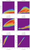 |
Fig. 14. Comparison of the properties of stellar orbits before (left column) and after (right column) buckling. The first row of plots shows the distribution of values of the amplitude in the z direction as a function of the amplitude in x. The second row shows the distribution of stars in the plane of frequency ratio and amplitude of oscillations in the x direction. The third row shows the distribution of stars in the fz–fx frequency plane. |
In the middle row of plots in Fig. 14 we show the distribution of stars in the plane of frequency ratio fz/fx and amplitude of oscillations in the x direction, ax. These maps contain similar information to the histograms on the right of Fig. 11 but now with the dependence on ax added. We see that while before buckling the distribution of frequency ratios is very wide, although somewhat narrower at smaller ax, after buckling it becomes very narrow with a very tight dependence on ax. All stars follow a very tight correlation between fz/fx and ax, with the exception of an additional small branch at fz, after/fx, after = 2 corresponding to banana-like orbits. Thus, when the dependence on ax is included, the range of occupied frequency ratios is even narrower for the buckled bar than the lower right histogram of Fig. 11 would suggest. We therefore confirm the result of Portail et al. (2015) who found that orbits of lower frequency ratios fz/fx occupy more inner parts of the boxy/peanut bar.
Further insight into the orbital structure of the bar before and after buckling can be obtained by plotting the distribution of stars in the fz–fx frequency plane at both times, as shown in the lower row of panels in Fig. 14. Before buckling, the distribution is much wider and the relation nonlinear, but after buckling, the relation between the two frequencies becomes very tight and linear. However, there is no strict proportionality between the two frequencies, that is the straight line does not cross the origin of the coordinate system. Instead, by fitting a straight line to the data we find that it can be very accurately approximated by

where fp turns out to be equal to the pattern speed of the bar, often denoted by Ωp, which in our case has the value of 2.5 Gyr−1. For fx, after between 5 and 20 Gyr−1 the formula (1) gives the values of fz, after/fx, after between 2 and 1.5, exactly as shown in the middle right panel of Fig. 14. We note that when plotting all the frequencies fz, after, fy, after and fx, after in a 3D plot rather than 2D, the frequencies lie along two narrow branches corresponding to the two peaks of fy, after/fx, after (see the lower left panel of Fig. 11), but when projected onto the fz–fx frequency plane they both fall on the same line.
The constant fp obtained when fitting formula (1) was simply a numerical value. However, it is natural to expect that it is not just a random number but rather some characteristic frequency of the system, which we indeed identify as the pattern speed of the bar. To make sure this is the case we made an independent calculation of orbital frequencies in the traditional cylindrical coordinate system and estimated the angular, radial, and vertical frequencies Ω, κ, and ν for the same selection of stars. We again found a very tight relation between Ω and ν. Since fx + fp = Ω and fz = ν, the relation (1) after buckling can be written in an even simpler way as

The results in terms of Ω, κ, and ν (not shown here) also confirm what was already demonstrated in Fig. 11, namely that most of the stars are on x1 orbits with κ/(Ω − Ωp) = 2 corresponding to the inner Lindblad resonance for the whole range of radii, both before and after buckling. Instead, the vertical resonance, ν/(Ω − Ωp) = fz/fx = 2 is populated only by a small fraction of stars before and after buckling (see the middle panels of Fig. 14). However, this resonance may have contributed to initiating the buckling, as we discuss below.
5. Discussion
Using N-body simulations we have studied the buckling instability in a barred galaxy similar to the Milky Way. The initial parameters of the model composed of an exponential disk embedded in a spherical dark matter halo were adjusted so that the bar forms slowly. The buckling event, occurring after 4.5 Gyr from the start of the simulation, is however quite violent and lasts only a fraction of a gigayear. We measured different properties of the buckling bar, including the mean acceleration, velocity, and distortion in the vertical direction both as a function of radius and in the face-on projection. We then studied the orbital structure of the bar before and after buckling determining the apocenters and frequencies of the stellar orbits supporting the bar that undergo buckling. The key result of this study is the discovery of a very tight relation between the frequency of stellar oscillations along the bar and in the vertical direction. The relation explains the dependence of the frequency ratio on radius in boxy/peanut bars found earlier in the literature. Still, the exact origin of the relation remains unclear.
We can however offer a tentative view on the nature of buckling instability using the results presented here. In Fig. 7 we show maps of the mean distortion of the stellar particles in the face-on view. In the initial stage of buckling, at t < 4.5 Gyr (second row of plots in Fig. 7) there appears a distortion with strong positive values at both ends of the bar, with maxima around x = ±6 kpc, and negative distortion oriented approximately perpendicular to the bar. This configuration is stationary in the reference frame of the bar for about 0.2 Gyr, that is it rotates together with the bar. Such a distortion can be produced by banana-like orbits with typical apocenters around 6 kpc. We found that such orbits after buckling have frequencies consistent with the vertical resonance fz/fx = 2. This suggests that the initial distortion of the bar is probably caused by resonant trapping of x1 orbits that become banana-like orbits.
Such a distortion at time t0 can be approximated in the circular form as zd(R, θ, t0)=z0(R)cosmθ with m = 2. As discussed by Binney & Tremaine (2008) in the context of galactic warps (their Sect. 6.6.1), when neglecting the vertical velocity, the evolution of such a distortion at a given radius R can be described as a propagation of two kinematic bending waves with pattern speeds ωp = Ω ± ν/2 (a different symbol ωp is used here to distinguish them from the pattern speed of the bar, Ωp). After buckling, the orbits in our bar obey ν = 4Ω/3, so the two pattern speeds are Ω/3 (slow wave) and 5Ω/3 (fast wave). The maximum distortion associated with the fast wave winds up rather quickly, as shown in the third row of plots in Fig. 7. We may estimate the pitch angle α of the line of maximum height in the usual way as cotα = (5/3)RΔt|dΩ/dR| (Binney & Tremaine 2008). For Δt = 0.15 Gyr (the time difference between t = 4.5 and t = 4.65 Gyr, the stages shown in the second and third rows of Fig. 7) and R = 6 kpc we find the pitch angle α ∼ 30 deg, in qualitative agreement with the image shown in the third row of Fig. 7. On the other hand, the slow wave winds up much more slowly in the inner part of the bar, and in the outer part, at R = 6 − 7 kpc, it survives (lower row of Fig. 7) because it corotates with the bar as in this region Ω/3 ≈ Ωp.
The situation seems to be different in the case of the second buckling taking place between t = 6.5 and t = 8 Gyr. Although a similar pattern of distortion appears also in this case (see the upper row of panels in Fig. 8), it occurs only in the outer part of the bar, at R > 5 kpc, but survives much longer. Since the bar grows steadily in this time period (see Figs. 2 and 3), it seems that as new stars are captured by the bar they are at the same time or soon after trapped by the vertical resonance so that the pattern is sustained. This picture is confirmed by the observation that the distortion moves toward outer radii in time (Fig. 5). In the end, around t = 8 Gyr, this pattern also winds up leaving behind a much larger boxy/peanut shape.
We conclude that buckling instability is probably essentially driven by the vertical resonance of the x1 stellar orbits in the bar. The orbits trapped by the vertical resonance initiate the distortion of the bar which then evolves in the form of kinematic bending waves. In the inner part of the bar the waves wind up forming a boxy/peanut shape, which in the second buckling event is extended to larger radii. The details of this process certainly deserve further study.
Acknowledgments
Useful comments from the referee, Daniel Pfenniger, are gratefully acknowledged. This work was supported in part by the Polish National Science Center under grant 2013/10/A/ST9/00023.
References
- Abbott, C. G., Valluri, M., Shen, J., & Debattista, V. P. 2017, MNRAS, 470, 1526 [NASA ADS] [CrossRef] [Google Scholar]
- Athanassoula, E. 2003, MNRAS, 341, 1179 [NASA ADS] [CrossRef] [Google Scholar]
- Athanassoula, E. 2005, MNRAS, 358, 1477 [NASA ADS] [CrossRef] [Google Scholar]
- Athanassoula, E. 2013, in Secular Evolution of Galaxies, eds. J. Falcón-Barroso, & J. H. Knapen (Cambridge: Cambridge Univ. Press), 305 [Google Scholar]
- Athanassoula, E. 2016, in Galactic Bulges, eds. E. Laurikainen, R. Peletier, & D. Gadotti (Switzerland: Springer International Publishing) [Google Scholar]
- Berentzen, I., Shlosman, I., Martinez-Valpuesta, I., & Heller, C. H. 2007, ApJ, 666, 189 [NASA ADS] [CrossRef] [Google Scholar]
- Binney, J., & Spergel, D. 1982, ApJ, 252, 308 [NASA ADS] [CrossRef] [Google Scholar]
- Binney, J., & Tremaine, S. 2008, Galactic Dynamics, 2nd edn. (Princeton: Princeton Univ. Press) [Google Scholar]
- Bureau, M., Aronica, G., Athanassoula, E., et al. 2006, MNRAS, 370, 753 [NASA ADS] [CrossRef] [Google Scholar]
- Carpintero, D. D., & Aguilar, L. A. 1998, MNRAS, 298, 1 [NASA ADS] [CrossRef] [Google Scholar]
- Ceverino, D., & Klypin, A. 2007, MNRAS, 379, 1155 [NASA ADS] [CrossRef] [Google Scholar]
- Ciambur, B. C., Graham, A. W., & Bland-Hawthorn, J. 2017, MNRAS, 471, 3988 [NASA ADS] [CrossRef] [Google Scholar]
- Combes, F., & Sanders, R. H. 1981, A&A, 96, 164 [NASA ADS] [Google Scholar]
- Combes, F., Debbasch, F., Friedli, D., & Pfenniger, D. 1990, A&A, 233, 82 [NASA ADS] [Google Scholar]
- Debattista, V. P., Carollo, C. M., Mayer, L., & Moore, B. 2004, ApJ, 604, L93 [NASA ADS] [CrossRef] [Google Scholar]
- Debattista, V. P., Mayer, L., Carollo, C. M., et al. 2006, ApJ, 645, 209 [NASA ADS] [CrossRef] [Google Scholar]
- Deibel, A. T., Valluri, M., & Merritt, D. 2011, ApJ, 728, 128 [NASA ADS] [CrossRef] [Google Scholar]
- Erwin, P., & Debattista, V. P. 2016, ApJ, 825, L30 [NASA ADS] [CrossRef] [Google Scholar]
- Erwin, P., & Debattista, V. P. 2017, MNRAS, 468, 2058 [NASA ADS] [CrossRef] [Google Scholar]
- Gajda, G., Łokas, E. L., & Athanassoula, E. 2016, ApJ, 830, 108 [CrossRef] [Google Scholar]
- Gajda, G., Łokas, E. L., & Athanassoula, E. 2017, ApJ, 842, 56 [NASA ADS] [CrossRef] [Google Scholar]
- Gajda, G., Łokas, E. L., & Athanassoula, E. 2018, ApJ, 868, 100 [NASA ADS] [CrossRef] [Google Scholar]
- Hopkins, P. F. 2015, MNRAS, 450, 53 [NASA ADS] [CrossRef] [Google Scholar]
- Hopkins, P. F., Wetzel, A., Kereš, D., et al. 2018, MNRAS, 480, 800 [NASA ADS] [CrossRef] [Google Scholar]
- Khoperskov, S., Di Matteo, P., Gerhard, O., et al. 2019, A&A, 622, L6 [NASA ADS] [CrossRef] [EDP Sciences] [Google Scholar]
- Li, Z.-Y., Ho, L. C., & Barth, A. J. 2017, ApJ, 845, 87 [NASA ADS] [CrossRef] [Google Scholar]
- Łokas, E. L. 2018, ApJ, 857, 6 [NASA ADS] [CrossRef] [Google Scholar]
- Łokas, E. L. 2019, A&A, 624, A37 [NASA ADS] [CrossRef] [EDP Sciences] [Google Scholar]
- Łokas, E. L., Athanassoula, E., Debattista, V. P., et al. 2014, MNRAS, 445, 1339 [NASA ADS] [CrossRef] [Google Scholar]
- Łokas, E. L., Ebrová, I., del Pino, A., et al. 2016, ApJ, 826, 227 [NASA ADS] [CrossRef] [Google Scholar]
- Martinez-Valpuesta, I., Shlosman, I., & Heller, C. 2006, ApJ, 637, 214 [NASA ADS] [CrossRef] [Google Scholar]
- Merritt, D., & Hernquist, L. 1991, ApJ, 376, 439 [NASA ADS] [CrossRef] [Google Scholar]
- Merritt, D., & Sellwood, J. A. 1994, ApJ, 425, 551 [NASA ADS] [CrossRef] [Google Scholar]
- Merritt, D., & Valluri, M. 1999, ApJ, 118, 1177 [NASA ADS] [CrossRef] [Google Scholar]
- Miller, R. H., Prendergast, K. H., & Quirk, W. J. 1970, ApJ, 161, 903 [NASA ADS] [CrossRef] [Google Scholar]
- Miralda-Escudé, J., & Schwarzschild, M. 1989, ApJ, 339, 752 [NASA ADS] [CrossRef] [Google Scholar]
- Miwa, T., & Noguchi, M. 1998, ApJ, 499, 149 [NASA ADS] [CrossRef] [Google Scholar]
- Navarro, J. F., Frenk, C. S., & White, S. D. M. 1997, ApJ, 490, 493 [NASA ADS] [CrossRef] [Google Scholar]
- Noguchi, M. 1996, ApJ, 469, 605 [NASA ADS] [CrossRef] [Google Scholar]
- Ostriker, J. P., & Peebles, P. J. E. 1973, ApJ, 186, 467 [NASA ADS] [CrossRef] [Google Scholar]
- Papaphilippou, Y., & Laskar, J. 1996, A&A, 307, 427 [NASA ADS] [Google Scholar]
- Patsis, P. A., & Harsoula, M. 2018, A&A, 612, A114 [NASA ADS] [CrossRef] [EDP Sciences] [Google Scholar]
- Patsis, P. A., Skokos, Ch, & Athanassoula, E. 2002, MNRAS, 337, 578 [NASA ADS] [CrossRef] [Google Scholar]
- Peschken, N., & Łokas, E. L. 2019, MNRAS, 483, 2721 [NASA ADS] [CrossRef] [Google Scholar]
- Pfenniger, D., & Friedli, D. 1991, A&A, 252, 75 [NASA ADS] [Google Scholar]
- Portail, M., Wegg, C., & Gerhard, O. 2015, MNRAS, 450, L66 [NASA ADS] [CrossRef] [Google Scholar]
- Raha, N., Sellwood, J. A., James, R. A., & Kahn, F. D. 1991, Nature, 352, 411 [NASA ADS] [CrossRef] [Google Scholar]
- Savchenko, S. S., Sotnikova, N. Ya., Mosenkov, A. V., Reshetnikov, V. P., & Bizyaev, D. V. 2017, MNRAS, 471, 3261 [NASA ADS] [CrossRef] [Google Scholar]
- Smirnov, A. A., & Sotnikova, N. Y. a. 2019, MNRAS, 485, 1900 [CrossRef] [Google Scholar]
- Springel, V. 2005, MNRAS, 364, 1105 [NASA ADS] [CrossRef] [Google Scholar]
- Springel, V., Yoshida, N., & White, S. D. M. 2001, New Astron., 6, 79 [Google Scholar]
- Toomre, A. 1966, Geophys. Fluid Dyn., 111 [Google Scholar]
- Valluri, M., & Merritt, D. 1998, ApJ, 506, 686 [NASA ADS] [CrossRef] [Google Scholar]
- Valluri, M., Debattista, V. P., Quinn, T., & Moore, B. 2010, MNRAS, 403, 525 [CrossRef] [Google Scholar]
- Valluri, M., Debattista, V. P., Quinn, T. R., Roškar, R., & Wadsley, J. 2012, MNRAS, 419, 1951 [NASA ADS] [CrossRef] [Google Scholar]
- Valluri, M., Shen, J., Abbott, C., & Debattista, V. P. 2016, ApJ, 818, 141 [NASA ADS] [CrossRef] [Google Scholar]
- Villa-Vargas, J., Shlosman, I., & Heller, C. 2010, ApJ, 719, 1470 [NASA ADS] [CrossRef] [Google Scholar]
- Voglis, N., Harsoula, M., & Contopoulos, G. 2007, MNRAS, 381, 757 [NASA ADS] [CrossRef] [Google Scholar]
- Weiland, J. L., Arendt, R. G., Berriman, G. B., et al. 1994, ApJ, 425, L81 [NASA ADS] [CrossRef] [Google Scholar]
- Widrow, L. M., & Dubinski, J. 2005, ApJ, 631, 838 [NASA ADS] [CrossRef] [Google Scholar]
- Widrow, L. M., Pym, B., & Dubinski, J. 2008, ApJ, 679, 1239 [NASA ADS] [CrossRef] [Google Scholar]
- Yoshino, A., & Yamauchi, C. 2015, MNRAS, 446, 3749 [NASA ADS] [CrossRef] [Google Scholar]
All Figures
|
Fig. 1. Evolution of the shape of the stellar component in time. Upper panel: evolution of the axis ratios b/a (intermediate to longest axis) and c/a (shortest to longest axis). Lower panel: triaxiality parameter T = [1 − (b/a)2]/[1 − (c/a)2] and the bar mode A2. Measurements were made for stars within the radius of 2Rd. |
| In the text | |
|
Fig. 2. Profiles of the bar mode A2(R) at different times. |
| In the text | |
|
Fig. 3. Evolution of the profiles of the bar mode A2(R) over time. |
| In the text | |
|
Fig. 4. Evolution of velocity dispersions of the stellar component over time. Upper panel: velocity dispersions along the cylindrical radius σR and along the vertical direction σz while lower panel: ratio σz/σR. Measurements were made for stars within the radius of 2RD. |
| In the text | |
|
Fig. 5. Evolution of the profiles of the mean acceleration (upper panel), velocity (middle panel), and distortion of the positions of the stars (lower panel) along the vertical axis z. Positive quantities point along the angular momentum vector of the disk. |
| In the text | |
|
Fig. 6. Surface density distributions of the stellar component viewed edge-on before the first buckling (t = 4 Gyr), at the time of first buckling (t = 4.5, 4.65 and 5 Gyr), at the time of second buckling (t = 7.1 Gyr), and at the end of evolution (t = 10 Gyr). The surface density was normalized to the central maximum value in each case and the contours are equally spaced in logΣ with ΔlogΣ = 0.05. |
| In the text | |
|
Fig. 7. Face-on maps of the mean acceleration (left column), mean velocity (middle column), and mean distortion of the positions of the stars (right column) along the vertical direction at the time of the first buckling. The four rows of panels show the results for times t = 4, 4.5, 4.65, and 5 Gyr. |
| In the text | |
|
Fig. 8. Same as Fig. 7 but at the time of second buckling (upper row) and at the end of evolution (lower row). |
| In the text | |
|
Fig. 9. Example of a buckling orbit. The orbit is plotted in different colors in three time periods: before, during, and after buckling (from the left to the right panel) and in two projections: in the face-on and edge-on view (the top and bottom row, respectively). After buckling the star follows a regular, periodic, pretzel-like orbit with frequency ratio fz, after/fx, after = 7/4, that is it completes four oscillations in x for every seven oscillations in z. |
| In the text | |
|
Fig. 10. Evolution of the position of the star along the minor and major axes of the bar for the orbit shown in Fig. 9. The time range of interest was divided into three parts: before, during, and after buckling, indicated with different colors. |
| In the text | |
|
Fig. 11. Histograms of frequency ratios fy/fx (left column) and fz/fx (right column) before (upper row, blue) and after (lower row, red) buckling. |
| In the text | |
|
Fig. 12. Distribution of the stars in the plane of the frequency of the orbit along a given direction after buckling vs. the same frequency before buckling. Upper panel: results for the motion along z and lower panel: for the motion along x. The color coding in these 2D histograms and the following figures is such that the red corresponds to maximum occupation and violet to empty cells. |
| In the text | |
|
Fig. 13. Distribution of stars in the plane of frequency ratios fz, before/fx, before and fz, after/fx, after. |
| In the text | |
|
Fig. 14. Comparison of the properties of stellar orbits before (left column) and after (right column) buckling. The first row of plots shows the distribution of values of the amplitude in the z direction as a function of the amplitude in x. The second row shows the distribution of stars in the plane of frequency ratio and amplitude of oscillations in the x direction. The third row shows the distribution of stars in the fz–fx frequency plane. |
| In the text | |
Current usage metrics show cumulative count of Article Views (full-text article views including HTML views, PDF and ePub downloads, according to the available data) and Abstracts Views on Vision4Press platform.
Data correspond to usage on the plateform after 2015. The current usage metrics is available 48-96 hours after online publication and is updated daily on week days.
Initial download of the metrics may take a while.