| Issue |
A&A
Volume 629, September 2019
|
|
|---|---|---|
| Article Number | A51 | |
| Number of page(s) | 12 | |
| Section | Stellar structure and evolution | |
| DOI | https://doi.org/10.1051/0004-6361/201936002 | |
| Published online | 03 September 2019 | |
Spatially resolved X-ray study of supernova remnants that host magnetars: Implication of their fossil field origin
1
Anton Pannekoek Institute, University of Amsterdam, PO Box 94249, 1090 Amsterdam, The Netherlands
e-mail: This email address is being protected from spambots. You need JavaScript enabled to view it.
2
School of Astronomy and Space Science, Nanjing University, Nanjing 210023, PR China
3
GRAPPA, University of Amsterdam, PO Box 94249, 1090 Amsterdam, The Netherlands
4
SRON, Netherlands Institute for Space Research, Sorbonnelaan 2, 3584 Utrecht, The Netherlands
5
Department of Physics and Astronomy, University of Manitoba, Winnipeg, MB R3T 2N2, Canada
6
Dipartimento di Fisica e Chimica E. Segrè, Università degli Studi di Palermo, Palermo, Italy
7
INAF-Osservatorio Astronomico di Palermo, Palermo, Italy
Received:
1
June
2019
Accepted:
15
July
2019
Abstract
Magnetars are regarded as the most magnetized neutron stars in the Universe. Aiming to unveil what kinds of stars and supernovae can create magnetars, we have performed a state-of-the-art spatially resolved spectroscopic X-ray study of the supernova remnants (SNRs) Kes 73, RCW 103, and N49, which host magnetars 1E 1841−045, 1E 161348−5055, and SGR 0526−66, respectively. The three SNRs are O- and Ne-enhanced and are evolving in the interstellar medium with densities of > 1 − 2 cm−3. The metal composition and dense environment indicate that the progenitor stars are not very massive. The progenitor masses of the three magnetars are constrained to be < 20 M⊙ (11–15 M⊙ for Kes 73, ≲13 M⊙ for RCW 103, and ∼13 − 17 M⊙ for N49). Our study suggests that magnetars are not necessarily made from very massive stars, but originate from stars that span a large mass range. The explosion energies of the three SNRs range from 1050 erg to ∼2 × 1051 erg, further refuting that the SNRs are energized by rapidly rotating (millisecond) pulsars. We report that RCW 103 is produced by a weak supernova explosion with significant fallback, as such an explosion explains the low explosion energy (∼1050 erg), small observed metal masses (MO ∼ 4 × 10⁻² M⊙ and MNe ∼ 6 × 10⁻³ M⊙), and sub-solar abundances of heavier elements such as Si and S. Our study supports the fossil field origin as an important channel to produce magnetars, given the normal mass range (MZAMS < 20 M⊙) of the progenitor stars, the low-to-normal explosion energy of the SNRs, and the fact that the fraction of SNRs hosting magnetars is consistent with the magnetic OB stars with high fields.
Key words: ISM: supernova remnants / nuclear reactions, nucleosynthesis, abundances / stars: magnetars / pulsars: general
© ESO 2019
1. Introduction
Stars with mass ≳8 M⊙ end their lives with core-collapse (CC) supernova (SN) explosions (see Smartt 2009, for a review). Two products are left after the explosion: a compact object (a neutron star, or a black hole for the very massive stars) and a supernova remnant (SNR). Both products are important sources relevant to numerous physical processes. Since the two objects share a common progenitor and are born in a single explosion, studying them together will result in a better mutual understanding of these objects and their origin.
Magnetars are regarded as a group of neutron stars with extremely high magnetic fields (typically 1014 − 1015 G, see Kaspi & Beloborodov 2017, for a recent review and see references therein). To date, around 30 magnetars and magnetar candidates have been found in the Milky Way, Large Magellanic Cloud (LMC), and Small Magellanic Cloud (Olausen & Kaspi 2014). For historical reasons, these magnetars are categorised as anomalous X-ray pulsars and soft gamma-ray repeaters, based on their observational properties. However, the distinction between the two categories has blurred over the last 10–20 years. Unlike the classical rotational powered pulsars, this group of pulsars rotates slowly with periods of P ∼ 2–12 s, large period derivatives Ṗ ∼ 10−13 − 10−10 s−1, and are highly variable sources usually detected in X-ray and soft γ-ray bands. In recent years, the extremely slowly rotating pulsar 1E 161348−5055 (P = 6.67 h) in RCW 103 is also considered to be a magnetar, because some of its X-ray characteristics (e.g., X-ray outburst) are typical of magnetars (De Luca et al. 2006; Li 2007; D’Aì et al. 2016; Rea et al. 2016; Xu & Li 2019).
The origin of the high magnetic fields of magnetars is still an open question. There are two popular hypotheses: (1) a dynamo model involving rapid initial spinning of the neutron star (Thompson & Duncan 1993), (2) a fossil field model involving a progenitor star with strong magnetic fields (Ferrario & Wickramasinghe 2006; Vink & Kuiper 2006; Vink 2008; Hu & Lou 2009). The dynamo model predicts that magnetars are born with rapidly rotating proto-neutron stars (on the order of millisecond), which can power energetic SN explosions (or release most of the energy through gravitational waves, Dall’Osso et al. 2009). This group of neutron stars is expected to be made from very massive stars (Heger et al. 2005). The fossil field hypothesis predicts that magnetars inherit magnetic fields from stars with high magnetic fields. Nevertheless, for the fossil field model, there is still a dispute on whether magnetars originate preferentially from high-mass progenitors (> 20 M⊙, Ferrario & Wickramasinghe 2006, 2008) or less massive progenitors (Hu & Lou 2009).
Motivated by the questions about the origin of magnetars, we performed a study of a few SNRs that host magnetars. As the SNRs are born together with magnetars, studying them allows us to learn what progenitor stars and which kinds of explosion can create this group of pulsars. Therefore, we can use observations of SNRs to test the above two hypotheses.
In order to get the best constraints of the progenitor masses, explosion energies, and asymmetries of SNRs, we selected those SNRs showing bright, extended X-ray emission. Among the ten SNRs hosting magnetars (nine in Olausen & Kaspi 2014, and RCW 103), only four SNRs fall into this category. They are Kes 73, RCW 103, N49 (in the LMC), and CTB 109. CTB 37B is another SNR hosting a magnetar, but with an X-ray flux one order of magnitude fainter and with sub or near-solar abundances (Yamauchi et al. 2008; Nakamura et al. 2009; Blumer et al. 2019). Here we do not consider HB9, as the association between HB9 and the magnetar SGR 0501+4516 remains uncertain. Vink & Kuiper (2006) and Martin et al. (2014) have studied the overall spectral properties of SNRs Kes 73, N49, and CTB 109 and found that their SN explosions are not energetic. In this study, with RCW 103 included and CTB 109 excluded, we constrain the progenitor masses of the magnetars, provide spatial information about various parameters (such as abundances, temperature, density), and explore the asymmetries using a state-of-the-art binning method. We exclude the oldest member CTB 109 from our sample1. Therefore, our sample contains Kes 73, RCW 103, and N49, which host magnetars 1E 1841−045, 1E 161348−5055, and SGR 0526−66, respectively. Their ages have been well constrained, and the spectra of most regions could be well explained with a single thermal plasma model (see Sect. 3). The distance of Kes 73 is suggested to be 7.5–9.8 kpc using the HI observation by Tian & Leahy (2008) and 9 kpc using CO observation (Liu et al. 2017). Here we take the distance of 8.5 kpc for Kes 73. The distance of RCW 103 is taken to be 3.1 kpc according to the HI observation (Reynoso et al. 2004, the upper limit distance is 4.6 kpc). N49 in the LMC is at a distance of 50 kpc.
2. Data and method
2.1. Data
We retrieved Chandra data of three SNRs – Kes 73, RCW 103, and N49. Only observations with exposure longer than 15 ks are used. The observational information is tabulated in Table 1. The total exposures of the three SNRs are 152 ks, 107 ks, and 114 ks, respectively.
Observational information of SNRs that host magnetars.
We used CIAO software (vers. 4.9 and CALDB vers. 4.7.7)2 to reduce the data and extract spectrum. Xspec (vers. 12.9.0u)3 was used for spectral analysis. We also used DS94 and IDL (vers. 8.6) to visualize and analyze the data.
2.2. Adaptive binning method
In order to perform spatially resolved X-ray spectroscopy, we dissected the SNRs into many small regions and extracted the spectrum from each region in individual observations. We employed a state-of-the-art adaptive spatial binning method called the weighted Voronoi tessellations (WVT) binning algorithm (Diehl & Statler 2006), a generalization of the Cappellari & Copin (2003) Voronoi binning algorithm, to optimize the data usage and spatial resolution. The same method has been used to analyze the X-ray data of SNR W49B and study its progenitor star (Zhou & Vink 2018). The X-ray events taken from the event file are adaptively binned to ensure that each bin contains a similar number of X-ray photons. Therefore, the WVT algorithm allows us to obtain spectra across the SNRs with similar statistical qualities.
Firstly, for each SNR, we produce a merged 0.3–7.0 keV image from all observational epochs using the command merge_obs in CIAO. This merged image is subsequently used to generate spatial bins using the WVT algorithm. Since this study focuses on the plasmas of SNRs, we exclude the magnetars’ emission by removing circular regions with angular radii of 15″, 20″, and 5″ (radius to encircle over 95% of the photon energy below 3.5 keV), respectively, for Kes 73, RCW 103, and N49. We also exclude the pixels with an exposure short than 40% of the total exposure. For the three SNRs, the targeted counts in each bin are 6400, 10 000, and 6400, respectively, corresponding to signal-to-noise ratios (S/N) of 80, 100, and 80, respectively. We obtain 83, 293, and 96 bins within Kes 73, RCW 103, and N49, respectively. Because RCW 103 is bright and is the most extended SNR among the three SNRs, we use a larger S/N to increase the statistics of each bin and do not define the SNR boundary. For the other two SNRs, we manually defined the boundaries of SNRs in order to include all the X-ray photons located around the edges. The merged images and adaptively binned images are shown in Fig. 1.
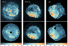 |
Fig. 1. Upper panels: merged Chandra images of three SNRs in the 0.3–7.0 keV energy band. Lower panels: adaptively binned images with the magnetars removed. The colorbars show the counts number per pixel (1″). |
Secondly, we extract spectra from each region (bin) in individual observations and jointly fit the spectra at each bin using a plasma model. From spectral fit, we obtain the best-fit parameters and their uncertainties at different bins. Finally, we study the distributions of the best-fit parameters across the SNRs and do further analysis (see Sect. 3).
3. Results
3.1. Spectral fit and density calculation
The X-ray emission of the three SNRs can be generally well fitted with an absorbed non-equilibrium ionization (NEI) plasma model, although some regions might need double components to improve the fit (Miceli et al., in prep.; Braun et al. 2019). The plasma model uses the atomic data in the ATOMDB code5 version 3.0.9. Using the single component model, we consider that the SN ejecta and the ambient media are mixed. An appropriate NEI model to describe the shocked plasma in young SNRs is the vpshock model, which describes an under-ionized plasma heated by a plane-parallel shock (Borkowski et al. 2001). This model allows us to fit the electron temperature kT, metal abundances, and the ionization timescale τ = ∫net, where ne is the electron density and t is the shock age (approximate SNR age). The Tuebingen-Boulder interstellar medium (ISM) absorption model tbabs is used for calculation of the X-ray absorption due to the gas-phase ISM, the grain-phase ISM, and the molecules in the ISM (Wilms et al. 2000). The solar abundances of Asplund et al. (2009) are adopted. We note that both single-temperature and multi-temperature components models are frequently used in SNRs. Two- or multi-temperature components are often needed for large extraction regions characterized by mixed ejecta and blast wave components, which as a result show a spatial variation of their spectral properties (such as the column density, the plasma temperature, the ionization timescale, or the gas density). Here we performed a state-of-the-art spatially resolved spectral analysis to address this complication. If two-temperature components are indeed needed everywhere in the SNR, the final best-fit parameters might be affected. Fitting a multi-thermal plasma with a single temperature causes a systematic error in the derived abundances. For example, an element whose strong lines have emissivities that peak at the derived temperature may have its abundance underestimated, while an element whose lines peak away from the derived temperature will have an overestimated abundance. Although more complicated models are indeed needed in many SNRs, the spectral decomposition is generally nonunique (Borkowski & Reynolds 2017) for many X-ray data and uncertainties are difficult to account for. The major reason for us to use the single thermal component is that it gives an adequately good fit to the spectra of most regions (in agreement with that pointed out by Borkowski & Reynolds 2017, for Kes 73).
Given the different spectral properties and environment of the three SNRs, the constrained metals are different. When the abundance of an element cannot be constrained, we fix it to the value of its environment (e.g., solar value in Kes 73 and RCW 103; LMC value in N49). For Kes 73, we fit the abundances of O (Ne tied to O), Mg, Si, S, and Ar. The soft X-rays of RCW 103 and N49 suffer less absorption, allowing us to fit the abundances of O and Fe (Ni tied to Fe), in addition to Ne, Mg, Si, and S. N49 is located in the LMC, so we used two absorption models to account for the Galactic and LMC absorption: tbabs (Gal) × tbvarabs (LMC). The H column density of the Galaxy towards N49 is fixed to 6 × 1020 cm−2 (Park et al. 2012) and the absorption in the LMC is varied. The LMC abundances of C (0.45), N (0.13), O (0.49), Ne (0.46), Mg (0.53), Si (0.87), S (0.41), Ar (0.62), and Fe (0.59) are taken from Hanke et al., (2010, see references therein). For other elements, an averaged value of 0.5 is assumed. The spectral fit results are summarized in the top part of Table 2.
Best-fit results and uncertainties.
The density is estimated based on an assumption of the volume or geometry for the X-ray emitting plasma. For a uniform density and a shock compression ratio of four, mass conservation suggests that for shell-type SNR with a radius of R, the shell should have a thickness of approximately ΔR = 1/12R: 4πR2ΔR(4ρ0)=4π/3R3ρ0, where ρ0 is the ambient density. The shell geometry is used to estimate the mean density nH for a given bin, combining the normalization parameter in Xspec (norm = 10−14/(4πd2)∫nenHdV, where d is the distance, ne and nH are the electron and H densities in the volume V; ne = 1.2nH for fully ionized plasma). If the X-ray gas fills a larger fraction of the volume across the SNR (1/12 < f < 1), the derived nH ∝ f−1/2. So the assumed geometry only affects the nH by a factor of up to 3.5.
The centers of Kes 73, RCW 103, and N49 are taken to be ( ,
,  ), (
), ( ,
,  ), and (
 ,
,  ), respectively. The radii are
  ,
,  , and
, and  , respectively.
3.2. Distribution of parameters
Figures 2–4 show the spatial distributions of the best-fit parameters across the SNRs Kes 73, RCW 103, and N49, respectively, except that the density panels are obtained from the best-fit norm and a geometry assumption. These three figures provide such ample information that it cannot be fully discussed in this work. In this paper, we will focus on the temperature, metal content, environment, and asymmetries.
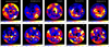 |
Fig. 2. Distribution of the best-fit parameters in Kes 73. The dashed circle indicates the outer boundary for density calculation. |
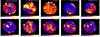 |
Fig. 3. Distribution of the best-fit parameters in RCW 103. The dashed circle indicates the outer boundary for density calculation. |
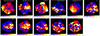 |
Fig. 4. Distribution of the best-fit parameters in N49. The dashed circle indicates the outer boundary for density calculation. |
We also plot the azimuthal and radial distribution of the best-fit parameters in Fig. 5. Here we briefly describe the distribution of some important parameters.
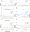 |
Fig. 5. Azimuthal and radial profiles of the best-fit parameters in Kes 73 (top), RCW 103 (middle), and N49 (bottom). The position angle increases counterclockwise from the north where the position angle is 0°. The SNR radius is RS. The profiles of the post-shock density are plotted with dashed lines. |
– Kes 73 (Fig. 2): There is a temperature variation across the SNRs (kT = 0.7–1.4 keV). The hottest plasma is located near the center of the SNR (kT up to 1.4 keV), while there is a cold (∼0.7–0.8 keV), broken-ring-like structure in the interior of the SNR (ring radius of  , ring centered at 18h41m18s, −04 ° 56′13″). Such temperature variation is roughly anti-correlated with the plasma density and the X-ray brightness (see Fig. 1).
There are abundance enhancements of the O (Ne tied to O), Mg, Si, and S elements. These elements show an east-west elongated structure, which is less clear in Ar, possibly because of the large uncertainties of abundance [Ar] and that the average [Ar] is less than one. Another possibility is a result of the degeneracy between [O] and NH in spectral fit, as the higher [O] at some regions show slightly lower NH.
Assuming that the gas is uniformly distributed in each bin, the average density is found to be  cm−3, suggesting an ambient density n0 = nH/4 ∼ 1.7 cm−3, consistent with the value obtained by Borkowski & Reynolds (2017, ∼2 cm−3). Such consistency indirectly supports that our geometry assumption is reliable to some extent. The density is enhanced in a broken-ring-like structure (∼10 cm−3), with an overall distribution similar to that of the X-ray brightness. Liu et al. (2017) suggested an interaction between the SNR and a molecular structure in the east, which may explain a larger column density NH there.
– RCW 103 (Fig. 3): The average temperature of the X-ray-emitting plasma is kT = 0.63 keV. The temperature distribution is nearly uniform, except for a higher temperature in some boundary regions (outside the main shock sphere, likely related to high-speed ejecta clumps or bad fit with single-temperature component model) and colder plasmas in the north.
We found that the O and Ne abundances are enhanced in RCW 103, while Borkowski & Reynolds (2017) obtained near solar abundances of them using the solar abundances of Grevesse & Sauval (1998), which give a 20% lower solar abundance of O compared to the abundance table we used (from Asplund et al. 2009). The [Ne] and [Mg] are more enhanced in the SNR interior, with an abundance gradient toward the outer part (see Fig. 5). The element O is enhanced in the southern regions ([O] ∼ 2 in Fig. 1) and [O] is largest in two inner-east bins, with [O] = 5 ± 1 and 4 ± 1, respectively. However, the NH values are also highest at the two bins. Considering a degeneracy between NH and [O] when fitting the soft X-ray emission, the [O] values at the two bins should be taken with caution.
The average density is 5.9 ± 0.2 cm−3. The density distribution has a barrel shape. The gas is greatly enhanced near the southeastern boundary (nH ∼ 9 cm−3;  to the SNR center,
  to the main shock boundary).
– N49 (Fig. 4): There is an overall temperature gradient from the west to the east, anti-correlated with the density. The hottest bin is in the west, with kT = 0.92 keV. The position is consistent with a protrusion as shown in Fig. 1, which is a Si and S-rich ([Si] = 1.15 and [S] = 2.3) ejecta knot. A detailed study of the knot can be found in Park et al. (2012).
The O, Ne, and S elements are enriched in N49 (mean [O] = 0.96, [Ne] = 1.2, and [S] = 1.6) compared to the LMC values. Similar to that in Kes 73 and RCW 103, the [Ne] distribution is centrally enhanced. Such an abundance gradient can be seen for O and Mg as well. Although the average abundances of Mg and Si are smaller than LMC values, the two elements appear more enhanced in the SNR interior. The distribution of S is asymmetrical, with higher abundance in the south.
The average density is 6.6 ± 0.3 cm−3. There is a clear density gradient from the southeast (∼10 cm−3) to the northwest (∼1 cm−3). This explains why the X-ray emission is brightened in the west.
3.3. Global parameters
Using the spectral fit results, we calculate a few important parameters related to the SNRs’ evolution and metals: gas mass Mgas, metal mass MX, SNR age t, and explosion energy E0. These results and the X-ray flux FX in the 0.5–7 keV band are listed in Table 2.
The masses of the X-ray-emitting gas Mgas are calculated with the fitted norm and assumed geometry. Using a similar method for density nH, we derived total gas masses of  in Kes 73, 12.8 ± 0.4 M⊙ in RCW 103, and
  in N49. We note that the assumed geometry of the density distribution affects the Mgas by a factor of a few. If the X-ray gas fills a larger fraction of the volume across the SNR (1/12 < f < 1), the derived Mgas could be slightly increased. Therefore, if f is assumed to be 1 (not likely for shell-type SNRs), we can derive the maximum limit of hot gas masses of
  ,
,  , and
, and  for Kes 73, RCW 103, and N49, respectively.
The metal masses are important parameters that can be used to compare with the supernova yields predicted from nucleosynthesis models and to test those models. We obtain the mass-weighted average abundances [X] and the observed ejecta mass MX as shown in the third part of Table 2. The abundance values are very similar to the bin-averaged abundances, so they are insensitive to the emission volume assumptions. The total masses of the metals are obtained by summing up the metal masses in each bin. For element X, the mass is obtained as ![Mathematical equation: $ M_{\mathrm{X}}=(([\mathrm{X}]-[\mathrm{X}]_{\mathrm{ISM}}) M_{\mathrm{gas}} f_{\mathrm{X}}^{\mathrm{m}} $](/articles/aa/full_html/2019/09/aa36002-19/aa36002-19-eq30.gif) , where the interstellar abundance is [X]ISM = 1 in our Galaxy and is equal to the LMC value for N49, and
, where the interstellar abundance is [X]ISM = 1 in our Galaxy and is equal to the LMC value for N49, and  is the mass fraction of the element in the gas.
The ages of the SNRs can be estimated from the electron temperature kT or from the ionization timescale τ. In the first method, the shock velocity is derived as vs = [16kTs/(3 μmH)]1/2, where mH is the mass of hydrogen atom and μ = 0.61 is the mean atomic weight for fully ionized plasma. The relation between the shock velocity and the electron temperature holds in case of temperature equilibrium between different particle species (and this can be the case, considering the relative high values of τ). The Sedov age is tsedov = 2Rs/(5vs). Using the averaged temperature kT in these SNRs, the ages of Kes 73, RCW 103, and N49 are found to be 2.4 kyr, 2.1 kyr, and 4.9 kyr, respectively. These values are consistent with those obtained in previous expansion measurements (for RCW 103 and Kes 73, respectively Carter et al. 1997; Borkowski & Reynolds 2017) and X-ray studies (Park et al. 2012; Kumar et al. 2014, for N49 and Kes 73, respectively). The X-ray emission of the three SNRs is characterized by under-ionized plasma. The shock age of an SNR t can be inferred from the ionization timescale τ = ∫net and the gas density nH = 1.2ne if the SNR is evolving in a uniform medium. We calculate a shock age in each bin and obtain the average age τshock (range) of 0.9 (0.4–1.8) kyr for Kes 73, 1.8 (> 0.6) kyr for RCW 103, and 8.0 (> 0.8) kyr for N49. By comparing the tshock values with tsedov values, one would find that the difference is smallest in RCW 103, but much larger in Kes 73 and N49, which are evolving in very inhomogeneous environment (see density distribution in Figs. 1 and 5). In a nonuniform medium, the tshock may deviate from the shock timescale. Moreover, the tshock values can be influenced by the geometry assumption. Therefore, we suggest that tsedov better represents the SNRs’ true age t.
The explosion energy of an SNR in the Sedov phase can be calculated using the Sedov-Taylor self-similar solution (Sedov 1959; Taylor 1950; Ostriker & McKee 1988):  , where n0 is the ambient density. We obtain
  erg,
erg,  erg, and
  erg for Kes 73, RCW 103, and N49, respectively. Here the radii are 5.5 pc, 3.9 pc, and 9.5 pc, respectively.
4. Discussion
The major goal of this paper is to explore which progenitor stars and which explosion mechanisms produce these SNRs and magnetars. The explosion energy and metal masses are two important parameters to characterize the explosion, while the distribution of metals provides information about the explosion (a)symmetries. On the other hand, the density distribution provide clues about the environment and even mass-loss histories of the progenitor star. In this section, we discuss these parameters in order to unveil the explosion and progenitor of magnetars.
4.1. Environment and clues about the progenitor
The density distribution is shown in Figs. 2–5, and gas masses are listed in Table 2. The masses of the X-ray-emitting gas are ∼46 M⊙ and ∼200 M⊙ in Kes 73 and N49, respectively, indicating that the gas is dominated by the ISM. Kes 73 is possibly interacting with molecular gas in the east (Liu et al. 2017), and N49 is interacting with molecular clouds in the southeast (Banas et al. 1997; Otsuka et al. 2010; Yamane et al. 2018). The inhomogeneous ambient medium significantly influences the X-ray morphology of the SNRs. As the density increases, the X-ray emission is brightened.
Massive stars launch strong winds during their main-sequence stage and could clear out low-density cavities (e.g., Chevalier 1999). If the massive star is in a giant molecular cloud, the maximum size of the molecular-shell bubble is linearly increased with the zero-age main-sequence (ZAMS) stellar mass: Rb = 1.22MZAMS/M⊙ − 9.16 pc (Chen et al. 2013). It is likely that the molecular shells found near the two SNRs were swept up by their progenitor winds. Therefore, taking the distance of the molecular gas to the SNR center (about the SNR radius), we can very roughly estimate the progenitor mass, which is 12 ± 2 M⊙ for Kes 73 and 15 ± 2 for N49. We note here that the Rb − MZAMS linear relationship was obtained from the winds of Galactic massive stars, and may not be valid for LMC stars with lower metallicity. Nevertheless, the derived mass of N49 agrees with the previous suggestion of an early B-type progenitor (MZAMS < 20 M⊙), which created a Strömgren sphere surrounding N49 (Shull et al. 1985).
The gas mass in RCW 103 is only ∼13 M⊙. Interestingly, the density distribution has a barrel shape with the shell at a distance of ∼3 pc to the center (Fig. 3). Between the position angle of ∼0° (north) and 100° (east), the density is reduced to 1/3–1/2 of that in other angles. In the opposite direction, the density is also relatively smaller. The density is largest in the southern and northern boundaries. This density distribution could explain why the SNR is elongated (more freely expanding) toward the low-density direction. It is likely that most of the X-ray-emitting gas has an ambient gas origin, because the density enhancement is consistent with the distribution of molecular gas in the southeast, northwest, and west (Reach et al. 2006). The existence of molecular gas with solar metallicity (Oliva et al. 1999) ∼3–4 pc away from the SNR center suggests that the progenitor is not very massive (MZAMS < 13 M⊙ if using the Rb − MZAMS relationship). Otherwise, the molecular gas would have been either dissociated by strong UV radiation or cleared out by fast main-sequence winds.
Although it is likely that the density distribution reflects the ambient medium, there is still a possibility that the lower density in the northeast and southwest is a result of the pre-SN winds. For example, a fast wind driven toward the northeast and southwest may clear out two lower density lobes. For a single star with MZAMS < 15 M⊙, its red super-giant winds are generally slow (∼10 km s−1) and the circumstellar bubble is small (< 1 pc Chevalier 2005), which cannot explain the low-density lobes. If the progenitor star was in a binary system, the accretion outflow could be fast and bipolar. However, there is no observational evidence so far to support the progenitor being a binary system.
4.2. Explosion mechanism implied from the observed metals
A common characteristic among the three SNRs is that all of them seem to be O- and Ne-enhanced, and there is no evidence of overabundant Fe (average abundance across the SNR). N49 reveals clear elevated [S], and Kes 73 shows slightly elevated [S], but [S] is sub-solar in most regions of RCW 103. Some regions with higher [O] show slightly lower NH. The degeneracy between the [O] and NH is difficult to distinguish using the current data. Future X-ray telescopes with better spectroscopic capability and higher sensitivity may resolve the O lines and solve this problem.
The abundance ratios and masses are a useful tool to investigate the SN explosion, since different progenitor stars and different explosion mechanisms result in distinct ejecta patterns. Figure 6 shows the predicted abundance ratios and yields of the ejecta as a function of the initial masses of the progenitor stars according to the one-dimensional CC SN nucleosynthesis models (Sukhbold et al. 2016, solar-metallicity model W18 for stars > 12 M⊙ and zero-metallicity model Z9.6 for 9–12 M⊙ by A. Heger)6. We hereafter compare the observed abundance ratios and metal masses of the SNRs with those predicted by the nucleosynthesis models for CC SN explosions (see Figs. 7 and 8).
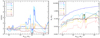 |
Fig. 6. Predicted abundance ratios (left) and yields (right) of the SN ejecta as a function of the progenitor masses based on the CC SN nucleosynthesis models by Sukhbold et al. (2016). The results of the 60 M⊙ and 120 M⊙ stars are out of range of the plot. |
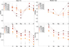 |
Fig. 7. Comparison of the observed abundance ratios (top) and metal masses (bottom) with the nucleosynthesis models for a range of massive stars (dots) in Sukhbold et al. (2016). For the predicted abundances in the upper panels, we take the shocked ISM into account by assuming that the SN ejecta are well mixed with the ISM (Mgas = 46 M⊙ for Kes 73 and Mgas = 12.8 M⊙ for RCW 103.) The [Si] and [S] in RCW 103 are subsolar, so the [Si]/[Mg] and [S]/[Mg] ratios do not provide useful information about the ejecta. |
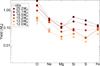 |
Fig. 8. Comparison of the metal masses in N49 with the nucleosynthesis models of Sukhbold et al. (2016). The masses of Mg, Si, and Fe are not plotted because they are lower than the typical values in the LMC. |
For the predicted abundances for Kes 73 and RCW 103, we take the shocked ISM into account by assuming that the SN ejecta are mixed with the ISM with solar abundances. As a result, the predicted abundance patterns are flatter than the pure ejecta values shown in Fig. 6. The ratios between elements with (sub)solar abundances do not provide information for the nucleosyntheis models, as we cannot extract ejecta components. Therefore, the Mg/Si ratio in Kes 73, and Si/Mg and S/Mg ratios in RCW 103 should not be taken seriously.
It is not always true that all the ejecta are mixed with the X-ray-bright ISM, especially for young SNRs. Nevertheless, we take the mass-averaged abundances across the SNRs to minimize the problems caused by the nonuniform distribution of the metals. Moreover, the observed metal masses compared to the model values in Fig. 7 provide a clue about the mixing level. For Kes 73 and RCW 103, the ISM masses are only a few to ten times the typical ejecta mass. The low metal abundances (< 2) indicate that the total metal masses are not very large and the progenitor star is probably not very massive, as the yields are generally increased with the stellar mass.
4.2.1. Kes 73
By fitting the abundance ratios with all the 95 models in Sukhbold et al. (2016, W18 and Z9.6, progenitor masses between 9 and 120 M⊙), we find that the five best-fit models for Kes 73 are the 11.75 (minimal  , see Fig. 7), 14.7, 14.5, 14.9, 14.8 M⊙ models (
 ). The observed ejecta masses of O and Ne in Kes 73 are small: MO = 0.14 ± 0.05 M⊙ and MNe = 3 ± 1 × 10⁻² M⊙. The ∼11 M⊙ model may explain the observed amount of O and Ne, but does not explain enhanced [O]/[Si] or [Ne]/[Si] ratios. Therefore, it is possible that not all metals are detectable in the X-ray band. If the reverse shock has not reached the SNR center, the inner part of the metals could remain cold and the total metal masses could be underestimated.
The location of reverse shock (likely showing a layer of enhanced metal abundances) is not identified in Kes 73 and RCW 103. A possible reason is that the total metal masses are indeed too small to emit strong X-ray lines. The other possibility is that the reverse shock has already reached the SNR center. The ratio of reverse shock radius Rr to forward shock radius Rs is related to the radial distribution of the circumstellar medium (nISM ∝ r−s) and ejecta nejecta ∝ r−n. For a uniform ambient medium s = 0 and an ejecta power-law index n = 7, the radius of the reverse shock Rr can be estimated using the solutions by Truelove & McKee (1999) and an assumed ejecta mass of 5 M⊙. In this case, the reverse shock should have reached the SNR center. In the s = 2 case, Katsuda et al. (2018a) obtained Rr/Rs ∼ 0.7.
Given the large uncertainties in Rr/Rs, we consider that the progenitor mass obtained from abundance ratios can better represent the true values for Kes 73. Nevertheless, the observed O and Ne masses allow us to exclude the progenitor models with a mass less than 11 M⊙.
In summary, the progenitor mass of Kes 73 is 11–15 M⊙, according to the model of Sukhbold et al. (2016). The mass of ∼12 M⊙ estimated from the molecular environment (see Sect. 4.1) is consistent with this range. Borkowski & Reynolds (2017) also obtained a relatively low mass of ≲20 M⊙ by comparing the observed metals with the nucleosynthesis model of Nomoto et al. (2013). Kumar et al. (2014) used two-temperature components to fit to the X-ray data and obtained abundance ratios overlapping ours, but they obtained a larger progenitor mass of ≳20 M⊙ based on earlier nucleosynthesis models (Woosley & Weaver 1995; Nomoto et al. 2006) and the Wisconsin cross sections for the photo-electric absorption model.
4.2.2. RCW 103
The progenitor model of 11.75 M⊙ is the best-fit model for O/Mg and Ne/Mg ratios in RCW 103 (see Fig. 7), and the five best models are 11.75, 17.6, 14.7, 12.0, and 17.4 M⊙ models. Here the Si/Mg and S/Mg ratios are not fitted.
The explosion energy of RCW 103 (∼1050 erg) is among the weakest in Galactic SNRs. Among the five well-fit models, two have progenitor masses ≤12 M⊙ and relatively weak explosion energy (E0 = 2.6 − 6.6 × 1050 erg), while the other models have a canonical explosion energy.
The total plasma mass of ∼13 M⊙ is only a few times larger than the expected ejecta mass for a CCSN from a normal explosion (≳5 M⊙). If all the ejecta have been heated by the shocks, we would expect to see high metal abundances. One possibility is that most of the ejecta are cool and not probed in the X-ray band for the normal SN explosion scenario. An alternative explanation is that the ejecta mass is indeed small because of significant fallback from a weak CCSN explosion (see discussion below).
The overall [Si] and [S] are subsolar, suggesting that overall Si and S production is low in RCW 103. Although a few Si/S-rich bins are detected in the SNRs (see Fig. 3), they may correspond to some pure ejecta knots (see also Frank et al. 2015, for Si and S ejecta knots). The distribution of [Mg] gives a clue to the missing Si/S problem. As shown in Figs. 3 and 5, the Mg element is oversolar in the SNR interior, but decreases to subsolar in the outer region. This implies that the heavier elements are distributed more in the inner regions compared to the lighter elements such as O and Ne. The Si and S materials may have smaller ejection velocities and the layers might not be heated by the reverse shock. A more extreme case is that the elements heavier than Mg may fall back to the compact objects due to a weak SN explosion.
The weak explosion energy of RCW 103 means that the total ejecta mass or the initial velocity of the ejecta should be smaller than normal SNRs. According to the simulation of a CCSN explosion invoking convective engine (Fryer et al. 2018), a weaker SN explosion results in a more massive neutron star and less ejecta due to fallback. Their simulation considered 15, 20, and 25 M⊙ cases. The weakest explosion (3.4 × 1050 erg) of a 15 M⊙ star creates a 1.9 M⊙ compact remnant, and more productions of O (0.29 M⊙) and Ne (0.064 M⊙) than observed in RCW 103. For a star more massive, a weak explosion would create a black hole. Therefore, we suggest that the progenitor star of RCW 103 has a mass of ≲13 M⊙, based on a comparison with the nucleosynthesis models, and the fact that the existence of nearby molecular shells disfavor a star more massive than 13 M⊙ (see Sect. 4.1). The two-temperature analysis of RCW 103 leads to a comparable progenitor mass and low explosion energy (Braun et al. 2019). However, the progenitor mass derived here is lower than the value of 18–20 M⊙ obtained from Frank et al. (2015) using an earlier nucleosynthesis model (Nomoto et al. 2006).
The low explosion energy, the small observed metal masses, and low abundances of heavier elements such as Si and S, consistently suggest that RCW 103 is produced by a weak SN explosion with significant fallback. It has been suggested that a supernova fallback disk may be a critical ingredient in explaining the very long spin period of 1E 161348−5055 in RCW 103 (De Luca et al. 2006; Li 2007; Tong et al. 2016; Rea et al. 2016; Xu & Li 2019). Our study supports this fallback scenario. In this case, the significant amount of fallback materials increase the mass of the compact object. Therefore, we predict that 1E 161348−5055 is a relatively massive neutron star.
4.2.3. N49
N49 is located in the LMC, while the W18 models are applied for stars with solar metallicity. Nevertheless, the lower metallicity mainly influences the mass loss of the stars but affects less the evolution in the core; therefore, the overall results from the core may be similar to those with solar metallicity for stars below 30 M⊙ (Sukhbold, priv. comm.).
The measured Si abundance of ∼0.6 is clearly lower than the typical value of 0.87 in the LMC (Hanke et al. 2010); this means the uncertainties of abundance ratios could be larger than the measurement values given the variation of the LMC abundance. Therefore, we only show a comparison of the measured metal masses with the nucleosynthesis model in Fig. 8. The 13 M⊙ model gives a relatively good fit to observed metal masses of O, Ne, and S. This puts a lower limit on the progenitor mass of N49, as lower mass stars produce less of these metals. The nucleosynthesis models predict that the 15–17 M⊙ stars produce abundance patterns with enhanced O and Ne relative to Si, and also enhanced S relative to O (see Fig. 6), which is the case for N49. Although a ∼26 M⊙ star may also produce these abundance patterns, it is not very likely to be the progenitor of N49 as its SN yields would be over one order of magnitude larger than the observed metal masses. Therefore, it is likely that N49 has a progenitor with a mass between 13 and 17 M⊙. This is consistent with the suggestion that N49 has an early B-type progenitor (Shull et al. 1985), while the progenitor mass obtained by Park et al. (2003) is larger (≳25 M⊙) based on enhanced Mg (not as enhanced here) and a comparison with an earlier nucleosynthesis model (Thielemann et al. 1996).
4.3. Implication for the formation of the magnetars
The progenitors of the three magnetars have the stellar masses of < 20 M⊙ (11–15 M⊙ for Kes 73, ≲13 M⊙ for RCW 103 and ∼13 − 17 M⊙ for N49), consistent with B type stars rather than more massive O type stars. The relatively low-mass progenitor stars of these three SNRs are also supported by Katsuda et al. (2018b, MZAMS < 15 M⊙), based on elemental abundances in the literature. Therefore, magnetars are not all necessarily made from very massive stars.
While there is so far no consensus on magnetar progenitors, there is evidence that some of them originate from very massive progenitors (MZAMS > 30 M⊙, see Safi-Harb & Kumar 2013, and references therein). A piece of evidence for very massive progenitors comes from the study of the magnetar CXO J164710.2−455216 in the massive star cluster Westerlund 1. The age and the stars of the stellar cluster suggest that the progenitor star of this magnetar has an initial mass of over 40 M⊙ (Muno et al. 2006). However, Aghakhanloo et al. (2019) reduced the distance of the cluster from 5 kpc to ∼3.2 kpc using Gaia data release 2 parallaxes. This revises the progenitor mass of the magnetar to 25 M⊙. Another magnetar, SGR 1806−20, in a massive star cluster was likely created by a star with a mass greater than 50 M⊙ (Figer et al. 2005). On the other hand, there is evidence that magnetars and high magnetic field pulsars are from lower mass stars, in addition to the three magnetars studied here. The SNR Kes 75 that hosts a high magnetic field pulsar J1846−0258 (but shows magnetar-like bursts, Gavriil et al. 2008) was considered to have a Wolf-Rayet progenitor (Morton et al. 2007). However, the existence of a molecular shell surrounding it suggests a progenitor mass of 12 ± 2 M⊙ for Kes 75 (Chen et al. 2013). A similar low mass (8–12 M⊙) was obtained from the far-IR observations and a comparison to the nucleosynthesis models (Temim et al. 2019). Moreover, the magnetar SGR 1900+14 in a stellar cluster is suggested to have a progenitor mass of 17 ± 2 M⊙ (Davies et al. 2009).
Magnetars are likely made from stars that span a large mass range. According to current knowledge about Galactic magnetars with progenitor information, most magnetars, though not all of them, seem to result from stars with < 20 M⊙. Among the three magnetars in our study, N49 seems to have a higher progenitor mass (13–17 M⊙) than RCW 103 (≲13 M⊙).
The SN explosion energies of the three magnetars are not very high, ranging from 1050 erg to ∼1.7 × 1051 erg, supporting the possibility that their SN explosions were not significantly powered by rapidly spinning magnetars. Particularly, RCW 103, the remnant hosting an ultra-slow magnetar with a rotational period of P = 6.67 h, resulted from a weak explosion with energy an order of magnitude lower than the canonical value. The SNR CTB 37B that hosts CXOU J171405.7−381031 also resulted from a weak explosion (1.8 ± 0.6 × 1050 erg, Blumer et al. 2019). Furthermore, CTB 109 (hosting 1E 2259+586) has a normal (Sasaki et al. 2004; Vink & Kuiper 2006) or even low explosion energy (2–5 × 1050 erg, see Sánchez-Cruces et al. 2018, for a recent measurement and see references therein). The low-to-normal SN explosion energy appears to be a common property of the known magnetar-SNR systems with extended thermal X-ray emission.
As pointed out in an earlier paper by Vink & Kuiper (2006), the relatively low or canonical explosion energy does not suggest that these three magnetars were born with very rapidly spinning millisecond pulsars. The rotational energy of a neutron star is Erot ≈ 3 × 1052(P/1 ms)−2 erg. A rapidly spinning magnetar loses its rotational energy quickly (∼10–100 s, Thompson et al. 2004). During the first few weeks, the magnetar energy goes into accelerating and heating the ejecta as the SN is optically thick, and at a later stage, the energy is released through radiation (Woosley 2010). This suggests that millisecond magnetars can lose some of their energies to the SN kinetic energies (∼40% in the model by Woosley 2010, but this fraction could be highly uncertain). Dall’Osso et al. (2009) proposed that gravitational waves might also take away the magnetar energy. The quickly rotating millisecond magnetar is regarded as a likely central engine for Type I superluminous supernovae (e.g., Woosley 2010; Kasen & Bildsten 2010). According to both theoretical studies and observations, superluminous SNe powered by millisecond magnetars should have significantly enhanced kinetic energies (2–10 × 1051 erg, Nicholl et al. 2017; Soker & Gilkis 2017). The three SNRs studied in this paper, in addition to CTB 109 and CTB 37B, have much lower kinetic energies than those of Type I superluminous SNe, indicating that their origin is different.
The distribution of the metals reveals some asymmetries: Kes 73 likely has enhanced O, Ne, and Mg abundances in the east (but could also be a result of the degeneracy between [O] and NH in spectral fit), RCW 103 shows enhanced O abundance in the south, and N49 shows clearly enhanced O, Ne, and Mg, Si toward the east, and enhanced S in the south. The element distributions are not always anti-correlated with the density, so the dilution due to the ejecta–gas mixing cannot be the main reason for the observed asymmetries, especially for Kes 73 and RCW 103. The nonuniform ejecta distributions reflect that the SN explosions should be aspherical to some extent.
With the above information, we can distinguish the two hypotheses about the origin of magnetars: dynamo origin or fossil field origin. The dynamo model predicts that the SN explosion is energized by the millisecond pulsar, which has been ruled out for the three magnetars discussed in this paper. Furthermore, the rapidly rotating stars are generally made from very massive stars (≤3 ms pulsars from 35 M⊙ stars, Heger et al. 2005). The SN rate is ≲5% for stars with an initial mass > 30 M⊙ and ∼10% for stars > 20 M⊙ (Sukhbold et al. 2016). These very massive stars are suggested to collapse to form black holes rather than neutron stars (Fryer 1999; Smartt 2009). Therefore, it is likely that only a small fraction of magnetars may be formed through this dynamo channel. We obtain a normal mass range (MZAMS < 20 M⊙) for the progenitor stars of the three magetars, further disfavoring the dynamo scenario for them.
The fossil field origin appears to be a natural explanation for magnetars. The magnetic field strengths of massive stars vary by a few orders of magnitude. The magnetic field detection rate is ∼7% for both B-type and O-type stars, with magnetic fields from several hundred Gauss to over 10 kG (e.g., Grunhut et al. 2012; Wade et al. 2014; Schöller et al. 2017). As to the origin of the strong magnetic fields in magnetic stars, the debates are almost the same as for magnetars: dynamo or fossil. The latter origin is supported from both theoretical studies and observations in recent years. Theoretical study of magnetic stars and magnetars has shown that stable, twisted magnetic fields (poloidal fields above the surface + internal toroidal fields) can have evolved from random initial fields (Braithwaite & Spruit 2004; Braithwaite 2009). Recent observations confirmed the fossil field origin (Neiner et al. 2015), because the dynamo origin would lead to a correlation between the magnetic field strength and stellar rotation speed, which is not observed. It is even suggested that the massive stars with higher magnetic fields rotate more slowly, likely due to magnetic braking (Shultz et al. 2018). Fossil magnetic fields of the stars are descendants from the seed fields of the parent molecular clouds (Mestel 1999). After the death of the stars, the neutron stars may also inherit the magnetic fields from these stars.
In our Galaxy, ten magnetars have been found in SNRs. Among the 295–383 known Galactic SNRs (Ferrand & Safi-Harb 2012; Green 2014, 2017), around 80% are of CC origin (0.81 ± 0.24, Li et al. 2011). This means that ∼3%−4% of CCSNRs are found to host magnetars. This fraction is slightly smaller than the incident fraction of magnetic OB stars with magnetic fields over a few hundred Gauss (∼7%), but consistent with the fraction of massive stars with higher fields (∼3% with B > 103 G, Schöller et al. 2017). Therefore, our study supports the fossil field origin as an important channel to produce magnetars, given the normal mass range (MZAMS < 20 M⊙) of the progenitor stars, the low-to-normal explosion energy of the SNRs, and the fraction of magnetars found in SNRs. Although our current study favors the fossil field origin and is against the dynamo origin for the three magnetars, we do not exclude the possibility that there might be more than one channel to create magnetars.
5. Conclusions
We have performed a spatially resolved X-ray study of SNRs Kes 73, RCW 103, and N49, aiming to learn how their magnetars are formed. Our study supports the fossil field as a probable origin of these magnetars. The main conclusions are summarized as follows:
-
The progenitor stars of the three magnetars are < 20 M⊙ (11–15 M⊙ for Kes 73, ≲13 M⊙ for RCW 103, and ∼13 − 17 M⊙ for N49). The progenitor masses are obtained using two methods: (1) a comparison of the metal abundances and masses with supernova nucleosynthesis models, (2) the nearby molecular shell that cannot be explained with very massive progenitor stars, which can launch strong main-sequence winds and create large low-density cavities. The two methods give consistent results.
-
Magnetars are likely made from stars that span a large mass range. According to current knowledge about Galactic magnetars, a good fraction of the magnetars seems to result from stars < 20 M⊙.
-
The explosion energies of the three SNRs span a large range, from 1050 erg to ∼1.7 × 1051 erg, further supporting that their SN explosions had not been significantly powered by millisecond magnetars.
-
A common characteristic among the three SNRs is that all of them are O- and Ne-enhanced, and there is no evidence of overabundant Fe (average value). The distribution of the metals reveals some asymmetries, reflecting that the SN explosions are probably aspherical to some extent. The next common property is that they are likely to be interacting with molecular structures swept up by winds of the progenitor stars.
-
We report that RCW 103 is produced by a weak SN explosion with significant fallback, given the low explosion energy (
 erg), the small observed metal masses (MO ∼ 4 × 10⁻² M⊙ and MNe ∼ 6 × 10⁻³ M⊙), and sub-solar abundances of heavier elements such as Si and S. This supports the fallback scenario in explaining the very long spin period of 1E 161348−5055.
 -
Our study supports the fossil field as a probable origin of many magnetars. The dynamo scenario, involving rapid initial spinning of the neutron star, is not supported given the normal mass range (MZAMS < 20 M⊙) of the progenitor stars, the low-to-normal explosion energy of the SNRs, and the large number of known Galactic magnetars. On the contrary, the fraction of CCSNRs hosting magnetars is consistent with the fraction of magnetic OB stars with high fields.
The X-ray emission in the western part of the SNR is almost totally absorbed, which means that only a fraction of the metals can be observed. For such an old SNR, the X-ray emission is highly influenced by the ISM. The spectra are dominated by two thermal components, and therefore the derived metal abundances and masses will be influenced by the assumed filling factors of the X-ray-emitting gas. Moreover, it might be difficult to constrain the age with good accuracy (e.g., 9–14 kyr, Vink & Kuiper 2006; Sasaki et al. 2013).
There is a large variation of abundance ratios at around 20 M⊙. As stated in Sukhbold et al. (2016) and Sukhbold & Woosley (2014), the transition from convective carbon core burning to radiative burning near the center at around this mass results in highly variable pre-SN core structures and, therefore, SN yields.
Acknowledgments
We thank Tuguldur Sukhbold for valuable discussions about his SN nucleosynthesis models. We also thank Hao Tong for helpful comments on the origin of magnetars. P.Z. acknowledges the support from the NWO Veni Fellowship, grant no. 639.041.647 and NSFC grants 11503008 and 11590781. S.S.H. acknowledges support from the Natural Sciences and Engineering Research Council of Canada (NSERC).
References
- Aghakhanloo, M., Murphy, J. W., Smith, N., et al. 2019, ArXiv e-prints [arXiv:1901.06582] [Google Scholar]
- Asplund, M., Grevesse, N., Sauval, A. J., & Scott, P. 2009, ARA&A, 47, 481 [NASA ADS] [CrossRef] [Google Scholar]
- Banas, K. R., Hughes, J. P., Bronfman, L., & Nyman, L. Å. 1997, ApJ, 480, 607 [NASA ADS] [CrossRef] [Google Scholar]
- Blumer, H., Safi-Harb, S., Kothes, R., Rogers, A., & Gotthelf, E. V. 2019, MNRAS, accepted [Google Scholar]
- Borkowski, K. J., & Reynolds, S. P. 2017, ApJ, 846, 13 [NASA ADS] [CrossRef] [Google Scholar]
- Borkowski, K. J., Rho, J., Reynolds, S. P., & Dyer, K. K. 2001, ApJ, 550, 334 [NASA ADS] [CrossRef] [Google Scholar]
- Braithwaite, J. 2009, MNRAS, 397, 763 [NASA ADS] [CrossRef] [Google Scholar]
- Braithwaite, J., & Spruit, H. C. 2004, Nature, 431, 819 [NASA ADS] [CrossRef] [PubMed] [Google Scholar]
- Braun, C., Safi-Harb, S., & Fryer, C. 2019, MNRAS, accepted [Google Scholar]
- Cappellari, M., & Copin, Y. 2003, MNRAS, 342, 345 [NASA ADS] [CrossRef] [Google Scholar]
- Carter, L. M., Dickel, J. R., & Bomans, D. J. 1997, PASP, 109, 990 [CrossRef] [Google Scholar]
- Chen, Y., Zhou, P., & Chu, Y.-H. 2013, ApJ, 769, L16 [NASA ADS] [CrossRef] [Google Scholar]
- Chevalier, R. A. 1999, ApJ, 511, 798 [NASA ADS] [CrossRef] [Google Scholar]
- Chevalier, R. A. 2005, ApJ, 619, 839 [NASA ADS] [CrossRef] [Google Scholar]
- D’Aì, A., Evans, P. A., Burrows, D. N., et al. 2016, MNRAS, 463, 2394 [NASA ADS] [CrossRef] [Google Scholar]
- Dall’Osso, S., Shore, S. N., & Stella, L. 2009, MNRAS, 398, 1869 [NASA ADS] [CrossRef] [Google Scholar]
- Davies, B., Figer, D. F., Kudritzki, R.-P., et al. 2009, ApJ, 707, 844 [NASA ADS] [CrossRef] [Google Scholar]
- De Luca, A., Caraveo, P. A., Mereghetti, S., Tiengo, A., & Bignami, G. F. 2006, Science, 313, 814 [NASA ADS] [CrossRef] [PubMed] [Google Scholar]
- Diehl, S., & Statler, T. S. 2006, MNRAS, 368, 497 [NASA ADS] [CrossRef] [Google Scholar]
- Ferrand, G., & Safi-Harb, S. 2012, AdSpR, 49, 1313 [Google Scholar]
- Ferrario, L., & Wickramasinghe, D. 2006, MNRAS, 367, 1323 [NASA ADS] [CrossRef] [Google Scholar]
- Ferrario, L., & Wickramasinghe, D. 2008, MNRAS, 389, L66 [NASA ADS] [CrossRef] [Google Scholar]
- Figer, D. F., Najarro, F., Geballe, T. R., Blum, R. D., & Kudritzki, R. P. 2005, ApJ, 622, L49 [NASA ADS] [CrossRef] [Google Scholar]
- Frank, K. A., Burrows, D. N., & Park, S. 2015, ApJ, 810, 113 [CrossRef] [Google Scholar]
- Fryer, C. L. 1999, ApJ, 522, 413 [NASA ADS] [CrossRef] [Google Scholar]
- Fryer, C. L., Andrews, S., Even, W., Heger, A., & Safi-Harb, S. 2018, ApJ, 856, 63 [CrossRef] [Google Scholar]
- Gavriil, F. P., Gonzalez, M. E., Gotthelf, E. V., et al. 2008, Science, 319, 1802 [NASA ADS] [CrossRef] [PubMed] [Google Scholar]
- Green, D. A. 2014, Bull. Astron. Soc. India, 42, 47 [NASA ADS] [Google Scholar]
- Green, D. A. 2017, VizieR Online Data Catalog: VII/278 [Google Scholar]
- Grevesse, N., & Sauval, A. J. 1998, Space Sci. Rev., 85, 161 [NASA ADS] [CrossRef] [Google Scholar]
- Grunhut, J. H., Wade, G. A., & MiMeS Collaboration 2012, ASP Conf. Ser., 465, 42 [Google Scholar]
- Hanke, M., Wilms, J., Nowak, M. A., Barragán, L., & Schulz, N. S. 2010, A&A, 509, L8 [NASA ADS] [CrossRef] [EDP Sciences] [Google Scholar]
- Heger, A., Woosley, S. E., & Spruit, H. C. 2005, ApJ, 626, 350 [NASA ADS] [CrossRef] [Google Scholar]
- Hu, R.-Y., & Lou, Y.-Q. 2009, MNRAS, 396, 878 [NASA ADS] [CrossRef] [Google Scholar]
- Kasen, D., & Bildsten, L. 2010, ApJ, 717, 245 [NASA ADS] [CrossRef] [Google Scholar]
- Kaspi, V. M., & Beloborodov, A. M. 2017, ARA&A, 55, 261 [NASA ADS] [CrossRef] [Google Scholar]
- Katsuda, S., Morii, M., Janka, H.-T., et al. 2018a, ApJ, 856, 18 [NASA ADS] [CrossRef] [Google Scholar]
- Katsuda, S., Takiwaki, T., Tominaga, N., Moriya, T. J., & Nakamura, K. 2018b, ApJ, 863, 127 [CrossRef] [Google Scholar]
- Kumar, H. S., Safi-Harb, S., Slane, P. O., & Gotthelf, E. V. 2014, ApJ, 781, 41 [CrossRef] [Google Scholar]
- Li, X.-D. 2007, ApJ, 666, L81 [NASA ADS] [CrossRef] [Google Scholar]
- Li, W., Chornock, R., Leaman, J., et al. 2011, MNRAS, 412, 1473 [NASA ADS] [CrossRef] [Google Scholar]
- Liu, B., Chen, Y., Zhang, X., et al. 2017, ApJ, 851, 37 [CrossRef] [Google Scholar]
- Martin, J., Rea, N., Torres, D. F., & Papitto, A. 2014, MNRAS, 444, 2910 [CrossRef] [Google Scholar]
- Mestel, L. 1999, Stellar Magnetism (Oxford: Oxford University Press) [Google Scholar]
- Morton, T. D., Slane, P., Borkowski, K. J., et al. 2007, ApJ, 667, 219 [NASA ADS] [CrossRef] [Google Scholar]
- Muno, M. P., Clark, J. S., Crowther, P. A., et al. 2006, ApJ, 636, L41 [NASA ADS] [CrossRef] [Google Scholar]
- Nakamura, R., Bamba, A., Ishida, M., et al. 2009, PASJ, 61, S197 [CrossRef] [Google Scholar]
- Neiner, C., Mathis, S., Alecian, E., et al. 2015, IAU Symp., 305, 61 [Google Scholar]
- Nicholl, M., Guillochon, J., & Berger, E. 2017, ApJ, 850, 55 [CrossRef] [Google Scholar]
- Nomoto, K., Tominaga, N., Umeda, H., Kobayashi, C., & Maeda, K. 2006, Nucl. Phys. A, 777, 424 [NASA ADS] [CrossRef] [Google Scholar]
- Nomoto, K., Kobayashi, C., & Tominaga, N. 2013, ARA&A, 51, 457 [NASA ADS] [CrossRef] [Google Scholar]
- Olausen, S. A., & Kaspi, V. M. 2014, ApJS, 212, 6 [NASA ADS] [CrossRef] [Google Scholar]
- Oliva, E., Moorwood, A. F. M., Drapatz, S., Lutz, D., & Sturm, E. 1999, A&A, 343, 943 [NASA ADS] [Google Scholar]
- Ostriker, J. P., & McKee, C. F. 1988, Rev. Mod. Phys., 60, 1 [NASA ADS] [CrossRef] [Google Scholar]
- Otsuka, M., van Loon, J. T., Long, K. S., et al. 2010, A&A, 518, L139 [NASA ADS] [CrossRef] [EDP Sciences] [Google Scholar]
- Park, S., Hughes, J. P., Burrows, D. N., et al. 2003, ApJ, 598, L95 [NASA ADS] [CrossRef] [Google Scholar]
- Park, S., Hughes, J. P., Slane, P. O., et al. 2012, ApJ, 748, 117 [NASA ADS] [CrossRef] [Google Scholar]
- Rea, N., Borghese, A., Esposito, P., et al. 2016, ApJ, 828, L13 [NASA ADS] [CrossRef] [Google Scholar]
- Reach, W. T., Rho, J., Tappe, A., et al. 2006, AJ, 131, 1479 [NASA ADS] [CrossRef] [Google Scholar]
- Reynoso, E. M., Green, A. J., Johnston, S., et al. 2004, PASA, 21, 82 [NASA ADS] [CrossRef] [Google Scholar]
- Safi-Harb, S., & Kumar, H. S. 2013, IAU Symp., 291, 480 [Google Scholar]
- Sánchez-Cruces, M., Rosado, M., Fuentes-Carrera, I., & Ambrocio-Cruz, P. 2018, MNRAS, 473, 1705 [CrossRef] [Google Scholar]
- Sasaki, M., Plucinsky, P. P., Gaetz, T. J., et al. 2004, ApJ, 617, 322 [NASA ADS] [CrossRef] [Google Scholar]
- Sasaki, M., Plucinsky, P. P., Gaetz, T. J., & Bocchino, F. 2013, A&A, 552, A45 [NASA ADS] [CrossRef] [EDP Sciences] [Google Scholar]
- Schöller, M., Hubrig, S., Fossati, L., et al. 2017, A&A, 599, A66 [NASA ADS] [CrossRef] [EDP Sciences] [Google Scholar]
- Sedov, L. I. 1959, Similarity and Dimensional Methods in Mechanics (New York: Academic Press) [Google Scholar]
- Shull, Jr., P., Dyson, J. E., Kahn, F. D., & West, K. A. 1985, MNRAS, 212, 799 [NASA ADS] [CrossRef] [Google Scholar]
- Shultz, M. E., Wade, G. A., Rivinius, T., et al. 2018, MNRAS, 475, 5144 [NASA ADS] [Google Scholar]
- Smartt, S. J. 2009, ARA&A, 47, 63 [NASA ADS] [CrossRef] [Google Scholar]
- Soker, N., & Gilkis, A. 2017, ApJ, 851, 95 [NASA ADS] [CrossRef] [Google Scholar]
- Sukhbold, T., & Woosley, S. E. 2014, ApJ, 783, 10 [NASA ADS] [CrossRef] [Google Scholar]
- Sukhbold, T., Ertl, T., Woosley, S. E., Brown, J. M., & Janka, H.-T. 2016, ApJ, 821, 38 [Google Scholar]
- Taylor, G. 1950, Proc. R. Soc. London Ser. A, 201, 159 [Google Scholar]
- Temim, T., Slane, P., Sukhbold, T., et al. 2019, ApJ, 878, L19 [CrossRef] [Google Scholar]
- Thielemann, F.-K., Nomoto, K., & Hashimoto, M.-A. 1996, ApJ, 460, 408 [NASA ADS] [CrossRef] [Google Scholar]
- Thompson, C., & Duncan, R. C. 1993, ApJ, 408, 194 [NASA ADS] [CrossRef] [Google Scholar]
- Thompson, T. A., Chang, P., & Quataert, E. 2004, ApJ, 611, 380 [NASA ADS] [CrossRef] [Google Scholar]
- Tian, W. W., & Leahy, D. A. 2008, ApJ, 677, 292 [NASA ADS] [CrossRef] [Google Scholar]
- Tong, H., Wang, W., Liu, X. W., & Xu, R. X. 2016, ApJ, 833, 265 [NASA ADS] [CrossRef] [Google Scholar]
- Truelove, J. K., & McKee, C. F. 1999, ApJS, 120, 299 [NASA ADS] [CrossRef] [Google Scholar]
- Vink, J. 2008, Adv. Space Rev., 41, 503 [CrossRef] [Google Scholar]
- Vink, J., & Kuiper, L. 2006, MNRAS, 370, L14 [NASA ADS] [CrossRef] [Google Scholar]
- Wade, G. A., Grunhut, J., Alecian, E., et al. 2014, IAU Symp., 302, 265 [Google Scholar]
- Wilms, J., Allen, A., & McCray, R. 2000, ApJ, 542, 914 [NASA ADS] [CrossRef] [Google Scholar]
- Woosley, S. E. 2010, ApJ, 719, L204 [NASA ADS] [CrossRef] [Google Scholar]
- Woosley, S. E., & Weaver, T. A. 1995, ApJS, 101, 181 [NASA ADS] [CrossRef] [Google Scholar]
- Xu, K., & Li, X.-D. 2019, ApJ, 877, 138 [CrossRef] [Google Scholar]
- Yamane, Y., Sano, H., van Loon, J. T., et al. 2018, ApJ, 863, 55 [CrossRef] [Google Scholar]
- Yamauchi, S., Ueno, M., Koyama, K., & Bamba, A. 2008, PASJ, 60, 1143 [CrossRef] [Google Scholar]
- Zhou, P., & Vink, J. 2018, A&A, 615, A150 [NASA ADS] [CrossRef] [EDP Sciences] [Google Scholar]
All Tables
All Figures
|
Fig. 1. Upper panels: merged Chandra images of three SNRs in the 0.3–7.0 keV energy band. Lower panels: adaptively binned images with the magnetars removed. The colorbars show the counts number per pixel (1″). |
| In the text | |
|
Fig. 2. Distribution of the best-fit parameters in Kes 73. The dashed circle indicates the outer boundary for density calculation. |
| In the text | |
|
Fig. 3. Distribution of the best-fit parameters in RCW 103. The dashed circle indicates the outer boundary for density calculation. |
| In the text | |
|
Fig. 4. Distribution of the best-fit parameters in N49. The dashed circle indicates the outer boundary for density calculation. |
| In the text | |
|
Fig. 5. Azimuthal and radial profiles of the best-fit parameters in Kes 73 (top), RCW 103 (middle), and N49 (bottom). The position angle increases counterclockwise from the north where the position angle is 0°. The SNR radius is RS. The profiles of the post-shock density are plotted with dashed lines. |
| In the text | |
|
Fig. 6. Predicted abundance ratios (left) and yields (right) of the SN ejecta as a function of the progenitor masses based on the CC SN nucleosynthesis models by Sukhbold et al. (2016). The results of the 60 M⊙ and 120 M⊙ stars are out of range of the plot. |
| In the text | |
|
Fig. 7. Comparison of the observed abundance ratios (top) and metal masses (bottom) with the nucleosynthesis models for a range of massive stars (dots) in Sukhbold et al. (2016). For the predicted abundances in the upper panels, we take the shocked ISM into account by assuming that the SN ejecta are well mixed with the ISM (Mgas = 46 M⊙ for Kes 73 and Mgas = 12.8 M⊙ for RCW 103.) The [Si] and [S] in RCW 103 are subsolar, so the [Si]/[Mg] and [S]/[Mg] ratios do not provide useful information about the ejecta. |
| In the text | |
|
Fig. 8. Comparison of the metal masses in N49 with the nucleosynthesis models of Sukhbold et al. (2016). The masses of Mg, Si, and Fe are not plotted because they are lower than the typical values in the LMC. |
| In the text | |
Current usage metrics show cumulative count of Article Views (full-text article views including HTML views, PDF and ePub downloads, according to the available data) and Abstracts Views on Vision4Press platform.
Data correspond to usage on the plateform after 2015. The current usage metrics is available 48-96 hours after online publication and is updated daily on week days.
Initial download of the metrics may take a while.