| Issue |
A&A
Volume 629, September 2019
|
|
|---|---|---|
| Article Number | A97 | |
| Number of page(s) | 13 | |
| Section | Cosmology (including clusters of galaxies) | |
| DOI | https://doi.org/10.1051/0004-6361/201935921 | |
| Published online | 11 September 2019 | |
COSMOGRAIL
XVIII. time delays of the quadruply lensed quasar WFI2033−4723⋆
1
Institute of Physics, Laboratory of Astrophysics, Ecole Polytechnique Fédérale de Lausanne (EPFL), Observatoire de Sauverny, 1290 Versoix, Switzerland
e-mail: vivien.bonvin@epfl.ch
2
Max Planck Institute for Astrophysics, Karl-Schwarzschild-Str. 1, 85740 Garching, Germany
3
Physik-Department, Technische Universität München, James-Franck-Straße 1, 85748 Garching, Germany
4
Institute of Astronomy and Astrophysics, Academia Sinica, 11F of ASMAB, No. 1, Section 4, Roosevelt Road, Taipei 10617, Taiwan
5
Subaru Telescope, National Astronomical Observatory of Japan, 650 N Aohoku Pl, Hilo 96720, Japan
6
Department of Physics, University of California, Davis, CA 95616, USA
7
STAR Institute, Quartier Agora – Allée du six Août 19c, 4000 Liège, Belgium
8
Kavli IPMU (WPI), UTIAS, The University of Tokyo, Kashiwa, Chiba 277-8583, Japan
9
National Astronomical Observatory of Japan, 2-21-1 Osawa, Mitaka, Tokyo 181-8588, Japan
10
Department of Physics and Astronomy, PAB, 430 Portola Plaza, Box 951547 Los Angeles, CA 90095, USA
11
Kavli Institute for Particle Astrophysics and Cosmology, Stanford University, 452 Lomita Mall, Stanford, CA 94035, USA
12
Fermi National Accelerator Laboratory, PO Box 500 Batavia, IL 60510, USA
13
Kavli Institute for Cosmological Physics, University of Chicago, Chicago, IL 60637, USA
14
Departamento de Ciencias Físicas, Universidad Andres Bello Fernandez Concha 700, Las Condes, Santiago, Chile
15
Centro de Astroingeniería, Facultad de Física, Pontificia Universidad Católica de Chile, Av. Vicuña Mackenna 4860, Macul 7820436 Santiago, Chile
16
Max-Planck-Institut für Astronomie, Königstuhl 17, 69117 Heidelberg, Germany
17
Las Cumbres Observatory Global Telescope, 6740 Cortona Dr., Suite 102, Goleta, CA 93111, USA
18
Department of Physics, University of California, Santa Barbara, CA 93106-9530, USA
19
Instituto de Física y Astronomía, Universidad de Valparaíso, Avda. Gran Bretaña 1111, Playa Ancha, Valparaíso 2360102, Chile
20
Millennium Institute of Astrophysics, Chile
21
Department of Physics, United States Naval Academy, 572C Holloway Rd., Annapolis, MD 21402, USA
22
Argelander-Institut für Astronomie, Auf dem Hügel 71, 53121 Bonn, Germany
23
Department of Astronomy, The Ohio State University, 140 West 18th Avenue, Columbus, OH 43210, USA
24
Center for Cosmology and Astroparticle Physics, The Ohio State University, 191 W. Woodruff Avenue, Columbus, OH 43210, USA
Received:
20
May
2019
Accepted:
11
June
2019
We present new measurements of the time delays of WFI2033−4723. The data sets used in this work include 14 years of data taken at the 1.2 m Leonhard Euler Swiss telescope, 13 years of data from the SMARTS 1.3 m telescope at Las Campanas Observatory and a single year of high-cadence and high-precision monitoring at the MPIA 2.2 m telescope. The time delays measured from these different data sets, all taken in the R-band, are in good agreement with each other and with previous measurements from the literature. Combining all the time-delay estimates from our data sets results in ΔtAB = 36.2+0.7−0.8 days (2.1% precision), ΔtAC = −23.3+1.2−1.4 days (5.6%) and ΔtBC = −59.4+1.3−1.3 days (2.2%). In addition, the close image pair A1-A2 of the lensed quasars can be resolved in the MPIA 2.2 m data. We measure a time delay consistent with zero in this pair of images. We also explore the prior distributions of microlensing time-delay potentially affecting the cosmological time-delay measurements of WFI2033−4723. Our time-delay measurements are not precise enough to conclude that microlensing time delay is present or absent from the data. This work is part of a H0LiCOW series focusing on measuring the Hubble constant from WFI2033−4723.
Key words: gravitational lensing: strong / galaxies: individual: WFI2033−4723 / cosmological parameters
Full light curves of the four data sets are only available at the CDS via anonymous ftp to cdsarc.u-strasbg.fr (130.79.128.5) or via http://cdsarc.u-strasbg.fr/viz-bin/cat/J/A+A/629/A97
© ESO 2019
1. Introduction
The flat-Λ cold dark matter (CDM) model, often labelled Standard Cosmological Model due to its ability to fit extremely well most of today’s cosmological observations, has recently been strengthened by the final update of the Planck satellite cosmic microwave background (CMB) observations (Planck Collaboration I 2018; Planck Collaboration VI 2018). However, a few sources of tension remain. One example is the predicted amplitude of overdensities in the Universe, characterized by the normalisation of the linear matter power spectrum σ8, that is in mild tension with direct measurements, such as the cosmic-shear analyses from the Kilo-Degree Survey (KiDS; Köhlinger et al. 2017; Troxel et al. 2018) and Hyper Suprime-Cam (HSC; Hikage et al. 2019). Similarly, Lyman-α measurements of Baryon Acoustic Oscillations at intermediate redshift (e.g. Bautista et al. 2017) are in a mild tension with the flat-ΛCDM predictions. More stringent is the measured expansion rate of the Universe, also called the Hubble constant H0, constrained through the observation of standard candles (e.g. Riess et al. 2019) that is in 4.4σ tension with the flat-ΛCDM predictions.
Whether such tensions result from underestimated systematic errors in at least one of the measurements, a statistical fluke, or point towards new physics beyond the Standard Model is currently a topic of discussion (see e.g. Mörtsell & Dhawan 2018; Poulin et al. 2019; Amendola et al. 2019; Capozziello et al. 2019; Pandey et al. 2019, for recent examples). There is however no simple, preferred alternative or extension to the flat-ΛCDM model that is clearly favoured by the existing data. In such a context, the way forward consists of improving the precision and accuracy of all measurements, as well as using alternative and independent techniques to estimate the conflicting cosmological parameters. Focusing on the Hubble constant, the so-called distance ladder method based on the cross-calibration of various distance indicators offers multiple routes towards H0 (see e.g. Cao et al. 2017; Jang et al. 2018; Dhawan et al. 2018; Riess et al. 2019, for recent updates). Galaxy clustering provides an alternative way to measure the Hubble constant independently from CMB measurements (e.g. DES Collaboration 2018; Kozmanyan et al. 2019), as well as the so-called “standard sirens” technique based on gravitational waves events (e.g. Abbott et al. 2017; Chen et al. 2018b; Feeney et al. 2019) or the observations of water vapour megamasers (e.g. Reid et al. 2013; Braatz et al. 2018).
An independent approach to directly measure H0 is to use time-delay cosmography. The idea, first proposed by Refsdal (1964), consists of measuring the time delay(s) between the luminosity variations of multiple images of a strongly gravitationally lensed source. Combined with careful modelling of the mass distribution of the lens galaxy, its surroundings and accounting of the mass along the line-of-sight, such measurements provide a direct way to constrain H0, which is nearly independent of any other cosmological parameters (see Treu & Marshall 2016; Suyu et al. 2018, for a review).
The H0LiCOW collaboration (Suyu et al. 2017) focuses on this method, using state-of-the-art software and techniques to carry out each step of the analysis. In 2017, H0LiCOW released its first results based on a blind analysis of the quadruply lensed quasar HE 0435−1223 (Sluse et al. 2017; Rusu et al. 2017; Wong et al. 2017; Bonvin et al. 2017; Tihhonova et al. 2018). Combined with two other strongly lensed systems analysed earlier (Suyu et al. 2010, 2014) and a fourth system analyzed recently (Birrer et al. 2019), it resulted in a 3% precision determination of the Hubble constant in a flat-ΛCDM universe,  km s−1 Mpc−1. This result, in mild tension with the CMB predictions but in excellent accord with the distance-ladder measurements, proves both the robustness of the method and its potential for deciding whether the discrepancies seen in H0 measurements are real or not.
The present paper is part of a series focusing on the analysis of the quadruply lensed quasar WFI2033−4723. It presents new time delay measurements based on monitoring data from the COSMOGRAIL collaboration taken between 2004 and 2018. In parallel, Sluse et al. (2019, hereafter H0LiCOW X) presents measurements of the spectroscopic redshifts of galaxies in the environment of WFI2033−4723. Rusu et al. (2019, hereafter H0LiCOW XII) focuses on the modelling of WFI2033−4723, taking into account the environment from H0LiCOW X and the time delays from the present work, to derive a value of the Hubble constant. Finally, Wong et al. (2019; hereafter H0LiCOW XIII) combines the time-delay distances from all the strongly lensed systems analysed so far by the H0LiCOW collaboration to infer cosmological parameters.
This manuscript is divided as follows: Sect. 2 presents the monitoring campaigns and the data reduction process that yield the light curves of the lensed images of the quasar. Section 3 presents the time-delay measurement framework, its application to our light curves and a series of robustness tests. Section 4 quantifies the effect of the microlensing time delay on the time-delay measurements. Section 5 summarizes our results and gives our conclusions.
2. Data sets
WFI2033−4723 is a bright, quadruply lensed quasar in a fold configuration (α(2000): 20h33m42.08s; δ(2000): −47°23′43.0″, Morgan et al. 2004). The most recent spectroscopic measurements of the lens and source redshifts are zd = 0.6575 (H0LiCOW X) and zs = 1.662 (Sluse et al. 2012), respectively.
WFI2033−4723 has been monitored since 2004 by the 1.2m Swiss Leonhard Euler telescope at the ESO La Silla Observatory in Chile, using the C2 instrument until October 2010 and the ECAM instrument since then, using the Rouge Genève filter, a modified version of the broad Bessel-R filter. Parallel observations took place since 2004 with the 1.3m Small and Moderate Aperture Research System (SMARTS) at the Cerro Tololo Inter-American Observatory (CTIO), using the KPNO R-band filter. From March to December 2017, WFI2033−4723 was also monitored daily with the MPIA 2.2 m telescope at the ESO La Silla Observatory using the WFI instrument with the ESO BB#Rc/162 filter. A summary of the observations is presented in Table 1, and the full light curves are available for download on the COSMOGRAIL website1 and on CDS. The main steps of the data reduction process are as follows:
Summary of the optical monitoring campaigns of WFI2033−4723.
1. Bias and flat exposures are taken on a regular basis. Master bias exposures are constructed to remove the additional bias level, and master flat exposures are constructed to correct for differences in the pixel sensitivity of the CCD detector. On the WFI exposures, fringes are occasionally observed. A fringe pattern correction is constructed by sigma clipping and stacking dithered exposures from the same epoch. The pattern is then subtracted from each individual science exposure.
2. The cleaned science exposures are sky-subtracted and aligned using standard sextractor and IRAF procedures. A number of reference stars are selected to construct an empirical Point Spread Function (PSF). Figure 1 presents a stacked exposure of the field-of-view of WFI2033−4723 from the WFI instrument. The stars selected for PSF construction are circled in green and labeled PSF 1 to PSF 6. Various choices of reference stars were explored, with the best results (i.e. the smallest residuals after deconvolution) being obtained for stars close in projection to the lens and slightly brighter than the lensed quasar images.
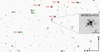 |
Fig. 1. Part of the field of view of WFI2033−4723 seen through the WFI instrument at the 2.2 m MPIA telescope. The field is a stack of 312 images with seeing ≤1″.4 and ellipticity ≤0.18, totalling ∼28 h of exposure. The insert represent a single, 320 s exposure of the lens in |

3. The quasar images are deconvolved, using the empirical PSF and the MCS deconvolution algorithm (Magain et al. 1998; Cantale et al. 2016). The deconvolution process separates the quasar light into two channels: (a) a collection of point sources representing the quasar images modelled following an analytical profile at a sub-pixel resolution, that we call the analytical channel and (b) a per-pixel fit of the light from the lens galaxy, other extended sources (such as the host galaxy of the quasar) as well as nearby perturbers, called the numerical channel. The flux of the point sources representing the quasar images is then normalised by an exposure-to-exposure normalisation coefficient, which is computed using a selection of reference stars in the field (circled in green and labelled N1 to N6 on Fig. 1) whose flux has been estimated in the same manner as the quasar images. This minimises the effect of systematic errors due to the deconvolution process and PSF mismatches. The normalised fluxes of each lensed quasar image are then combined for each observing epoch.
The light curves obtained from each instrument are presented in Fig. 2. The top panel presents the combined C2+ECAM data sets (the small gap in the 2010 season corresponding to the change of instrument), the middle panel presents the SMARTS data set and the bottom-left panel presents the WFI data set. Similar features are clearly visible across all light curves and data sets. A merger of all the data sets exhibits no discrepancies in the stacked light curves, provided an instrumental offset in magnitude between each data set. We note that the C2, SMARTS and ECAM data sets have been already partially discussed: Vuissoz et al. (2008) use three and a half years of data (from 2004 to mid-2007) to measure time delays and the Hubble constant with crude models, and Morgan et al. (2018) use the SMARTS, C2 and ECAM data up to 2016 to estimate the quasar accretion disk size from microlensing analysis. We emphasize that the data reduction process presented in this section and the time-delay analysis described in Sect. 3 are completely independent of these previous studies. The ECAM data set after 2016 and the entire WFI data set are presented for the first time in this work. The ambient quality of the observations are illustrated in the bottom right panel of Fig. 2. The WFI data set clearly stands out as the best in seeing, thanks to better dome seeing, a better instrument and flexible scheduling at the telescope.
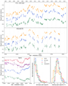 |
Fig. 2. WFI2033−4723 light curves from the four different instruments used in this work. Top panel: Euler data sets (C2+ECAM instruments), with the change occuring in October 2010, corresponding to the small gap visible in the 2010 season. Middle panel: SMARTS data set. Bottom left panel: WFI data set, where the A1 and A2 images were individually resolved thanks to superior image quality and longer exposure times. We note that different calibration stars were used for the different data sets, hence the differences in the relative magnitudes between the instruments. Bottom right panel: normalised distribution of the airmass and seeing of all the individual exposures in each data set. |
For the C2, ECAM and SMARTS data sets, our deconvolution scheme is not able to properly resolve the close pair of images A1 and A2. The two deconvolved images share flux even after deconvolution, and the structures in their light curves are clearly polluted by correlated noise. As the cosmological time delay between the A1 and A2 images is expected to be very small (Vuissoz et al. 2008), we chose instead to merge A1 and A2 into a single, virtual image A light curve. To do so, we sum the deconvolved A1 and A2 fluxes, and compute the joint uncertainty as the quadratic sum of the A1 and A2 individual uncertainties. For the WFI data set, the size of the instrument’s primary mirror (2.2 m) coupled to a longer exposure time with respect to the other instruments allows us to reach a sufficient signal-to-noise ratio to properly resolve the A1 and A2 images after deconvolution. An estimate of the time delay between A1 and A2 is given in Sect. 3. Having an extra light curve allows a third independent time-delay measurement to constrain the lens models. As such, it represents a crucial extra piece of information for time-delay cosmography.
3. Time-delay measurement
In this section, we measure the time delays for each of the individual data sets and combine them into a final time-delay estimate to be used at the lens modelling stage (see H0LiCOW XII). We start by giving a description of the framework used in this paper, emphasizing how the time-delay uncertainties are evaluated, before presenting our time-delay estimates and performing robustness checks to assess the quality of our measurements. Let us first recall the terminology used here, adopted from Tewes et al. (2013a), Bonvin et al. (2018, 2019).
– A point estimator is a method that returns the best time-delay estimates Δt = [Δtij] between two or more light curves, with i, j ∈ [A, B, C, …]. A point estimator depends on estimator parameters that impact its results, for example by controlling the smoothness of a fit.
– The intrinsic error is the dispersion of a point estimator when randomizing its initial state, such as the starting point of an iterative estimator (in our case an initial guess for the time delay). We note that this is different from the error we would get by varying the estimator parameters.
– A generative model of mock light curves is a process that draws simulated light curves that mimic as closely as possible the input data, but with known time delays. We apply our point estimators on a large set of these simulated light curves in order to estimate a point estimator’s uncertainties δt = [(δt+, δt−)ij]. Generative models, similarly to point estimators, depend on a set of generative model parameters that control the generation of the simulated light curves.
– A curve-shifting technique is the combination of a point estimator with a generative model. In the following, we call the curve-shifting technique parameters the joint point estimator and generative model parameters. With a chosen set of curve-shifting parameters, the point estimator can be used to estimate the time delays from the data and the generative model can be used to draw mock light curves with known time delays to assess the uncertainty of the point estimates.
– A Group G = [Eij], composed of independent time-delay estimates  , is the result of the application of a curve-shifting technique on a data set for a given choice of curve-shifting technique parameters.
– A Series S = [G1, …Gk, …, GN],k ∈ N, consists of multiple Groups that share the same data set and point estimator, but differ in their choice of curve-shifting technique parameters. Typically, a Series is a collection of Groups whose time-delay estimates are a priori equivalently probable, and thus can be combined or marginalised over.
3.1. PyCS formalism
We measure the time delays using the open-source PyCS software (Tewes et al. 2013a; Bonvin et al. 2016). PyCS is currently composed of two different point estimators.
– The free-knot splines estimator fits (i) a unique spline to model the intrinsic luminosity variations common to all the lensed images, and (ii) individual extrinsic splines to each light curve in order to model the microlensing magnification by compact objects in the lens galaxy. The time shifts between the light curves are optimised concurrently with the spline fits in an iterative process, following the BOK-splines algorithm of Molinari et al. (2004). The smoothness of the fit is controlled by the number of knots in the splines, which we represent by the initial (i.e. prior to the optimisation) temporal spacing between the knots, denoted η and ηml for the intrinsic and extrinsic splines, respectively. Special constraints on the knots position are denoted by ηpos and  .
.
– The regression difference estimator fits individual regressions through each light curve using Gaussian Processes. The regressions are then shifted in time with respect to each other, pair by pair. At each time step, the amount of variations of the difference of the two regressions is evaluated; to the smallest variability (the “flattest” difference curve) is associated the best time-delay point estimate. The estimator parameters consist of a choice of covariance kernel (and associated parameters) for the Gaussian Process. The regression difference estimator does not require any explicit modelling of the microlensing.
To assess the uncertainties of these two point estimators, PyCS implements a generative model for mock lensed quasar light curves. It takes as input (i) a model for the intrinsic luminosity variations of the quasar, (ii) models for the extrinsic variations of the individual light curves, (iii) the sampling and noise properties of the observations, and (iv) the true time delays to recover. The intrinsic and extrinsic variations are modelled after the best fit of the free-knot splines estimator on the real data. The sampling of the mock curves matches that of the real observations, and the noise is a combination of red and white noise calibrated on the real data (see Tewes et al. 2013a, for the details). Finally, the true time delays are randomly sampled over a range of values around the actual time delays measured on the real light curves. The dispersions of the point estimators’ results around the true delays of the mock light curves are used to estimate the uncertainties.
With two point estimators and one generative model, PyCS offers two different curve-shifting techniques. The two techniques are not completely independent as they share the same generative model, but offer a nice cross-validation of the results. Note that we are exploring a novel generative model in our robustness tests, as compared with previous work. When having access to multiple data sets from different instruments, like in the present case for WFI2033−4723, we chose to analyse the data sets independently from each other as long as they are each of sufficient quality to yield robust time-delay estimates. Proceeding this way is also better to fully extract the constraining power of each data set, since different data sets can be best fit with different estimator parameters due to their differences in sampling and photometric uncertainties. We explore the results obtained when combining the data sets as a robustness test in Sect. 3.4.
For each curve-shifting technique and each data set, we vary the curve-shifting technique parameters to obtain a Group of time-delay estimates. The exploration of the range of plausible curve-shifting parameters is done as follows. For a curve-shifting technique that uses the free-knot splines estimator, we use the same parameters for the point estimator and the generative model (recall that the generative model is based on a free-knot spline fit to the data), for simplicity. For a curve-shifting technique that uses the regression difference estimator, we use the same generative model parameters as the curve-shifting techniques based on the free-knot splines estimator. What constrains our choice of parameters for a point estimator is the intrinsic error it yields; we limit ourselves to the sets of parameters that yield an intrinsic error qualitatively much smaller than the smallest total uncertainty of the most precise curve-shifting technique we have. Although this might seem somewhat arbitrary, a large intrinsic error is a robust indicator that the point estimator either overfit or underfit the data, which is something we want to avoid.
The various Groups obtained by exploring the different plausible sets of curve-shifting technique parameters are then gathered in a Series. Each Group of the Series represents a plausible measurement of the time delays. If all the Groups have similar time-delay measurements (albeit with different uncertainties), we consider the most precise Group as our reference. However, if two or more Groups are in tension, keeping only the most precise one is not a good option as the tension might indicate a possible bias related to the choice of the curve-shifting parameters. Instead, we iteratively marginalise over the Groups in tension until that tension stays below a defined threshold, following the formalism presented in Sect. 4.1 of Bonvin et al. (2019). We adopt a fiducial threshold value of σthresh = 0.5 in this work. In practice, it means that once the most precise Group of the Series has been identified, its tensions with the remaining Groups are computed; the most precise Group for which the tension with the reference Group exceeds 0.5σ (if any) is selected, and the marginalisation (summation) of these two Groups become the new reference Group. The process is repeated until all the tensions drop below 0.5σ, or all the Groups are combined (which, in the present case, never happens). As the choice of σthresh = 0.5 might seem arbitrary, we explore the impact of varying this threshold in our robustness tests in Sect. 3.4.
In a first approach, exploring the curve-shifting technique parameters and combining the results as we do in this work can be done using a grid search followed by a weighted marginalisation over the results. Ideally, the exploration of the curve-shifting parameters would be performed in a full Bayesian framework, but this is currently too expensive computationally due to the time required to sample the results for a single set of curve-shifting parameters. Although not perfect, we deem our current formalism as more conservative than the previous time-delay measurements of the COSMOGRAIL collaboration (Bonvin et al. 2017; Courbin et al. 2018). Whether this formalism is too conservative or not is still an open – and complicated - question, that we will address in a forthcoming work (Millon et al., in prep.), in which we will go one step further towards a complete Bayesian analysis.
In the end, we have one Group of time-delay estimates for each data set and curve-shifting technique. The next step is to combine these Groups together. As stated earlier, the two curve-shifting techniques implemented in PyCS are not fully independent, so we chose to fully marginalise over their respective results. In practice, this translates into summing the normalised probability density distributions of each time-delay estimate for the free-knot splines and the regression difference estimator Groups, thus yielding a single Group for each data set. Finally, combining the results of the various data sets together can be done either by multiplying the respective probability density distributions or by marginalising over the individual results, if we assume that the time-delay measurements are or are not independent, respectively.
3.2. Application to WFI2033−4723
We now apply this formalism to the data sets presented in Sect. 2. For WFI2033−4723, we have four different data sets. In a similar fashion to Bonvin et al. (2018), we analyze these data sets independently from each other. However, we explore the results obtained by simultaneously fitting all of the data sets as a robustness test in Sect. 3.4.
The range of the curve-shifting technique parameters to explore must reflect the state of our knowledge about the data sets. For example, the light curves presented in Fig. 2 are a combination of the intrinsic luminosity variations of the quasar, common to all light curves, and individual extrinsic variations due to microlensing magnification by compact objects in the lens galaxy. Since the amount of microlensing magnification is a priori unknown, various microlensing models should be considered if the curve-shifting technique aims to model it explicitly. Similarly, there is no clear consensus on how to properly represent the intrinsic quasar luminosity variations; on long temporal scales, a damped random walk model gives good results (e.g. Kozłowski et al. 2010; Zu et al. 2013), whereas on short time scales it apparently predicts too much variability (e.g. Mushotzky et al. 2011; Kasliwal et al. 2015). Consequently, we adopt a data-driven approach and explore various choices for the parameters controlling the smoothness of the fit of the intrinsic and extrinsic variations.
The curve-shifting technique parameters used in this work are presented in Table 2. For each set of estimator parameters – 9 for the free-knot splines estimator and 5 for the regression difference estimator2, we obtain a Group of time-delay estimates, that we combine following the formalism presented in Sect. 3.1. We present the combined time-delay measurements for each data set in Fig. 3. We also present the two possible combinations of these time-delay measurements: (i) a marginalisation (labelled “sum” in the figure) and (ii) a multiplication (labelled “mult” in the figure). In addition to our own measurements, we report the time-delay measurements of Vuissoz et al. (2008) and Morgan et al. (2018), that use subsets of the data presented in this work. Both measurements are consistent with our work, although neither of them provide a direct measurement for the AC time delay; their AB and BC time delays are visible as smaller dots on Fig. 3. We note that Giannini et al. (2017) obtained light-curves of WFI2033−4723 taken with the 1.54 m Danish telescope at the ESO La Silla Observatory, as part of the MiNDSTEp collaboration. However, they do not provide time-delay estimates. We tried to apply PyCS to their data but varying the estimator and generative model parameters gave discrepant results with very large uncertainties. We conclude that the MiNDSTEp data set is not of sufficient quality to produce reliable time-delay estimates on its own, and thus we do not include it in our analysis.
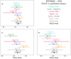 |
Fig. 3. WFI2033−4723 time-delay estimates. The colored points labelled “PyCS” represent the final time-delay estimates for each data set, obtained after combining the curve-shifting technique parameters following the marginalisation scheme presented in Sect. 3.1. The gray and black points, respectively labelled “PyCS-sum” and “PyCS-mult” represent the marginalisation and combination of the results obtained from the individual data sets. Indicated with small diamonds and dashed lines are the AB and BC delays taken from Morgan et al. (2018) and Vuissoz et al. (2008), respectively. The similar color between “PyCS -C2” and Vuissoz 2008 indicates that both measurement share the same data set, although less complete in the latter case (see Table 1). The values indicated above each measurement represent the 50th, 16th and 84th percentiles of the respective probability distributions. |
Overall, our measurements agree well with each other. To quantify that agreement, we compute the Bayes Factor, or evidence ratio F = ℋsame/ℋbias, following Marshall et al. (2006). The idea is to test which hypothesis is the most probable: either ℋsame that the time-delay measurements of each data set are all representing the same quantity – the cosmological time delays – or ℋbias that at least one measurement represents a biased measurement of the cosmological time delay, for example due to the presence of microlensing time delay (Tie & Kochanek 2018). F > 1 indicates that it is more probable for the time-delay measurements to not be significantly affected by systematic errors (or to be similarly biased). In such a case, a combination of the time-delays estimates such as the “PyCS-mult” should be favored over the marginalization of “PyCS-sum”. We test every possible combination of the individual time-delay estimates and find that F is always greater than 1. As it can be guessed from Fig. 3, the smallest Bayes Factor arises when comparing the AC delay of SMARTS and WFI, with  . The evidence ratios obtained when considering all the data sets independently are
  ,
,  and
and  , indicating that we should be able to use the combined “PyCS-mult” results of Fig. 3 without any loss of consistency.
We note that a Bayes Factor greater than one, showing that the individual measurements are mutually consistent, does not necessarily mean that there are no unaccounted random uncertainties affecting them. Rather, it means that the uncertainties of the individual measurement are large enough not to be significantly affected by unaccounted random error, or that similar systematic errors affect all our measurements. In the case of time-delay measurements, a potential albeit speculative source of error could be the microlensing time delay. A full description of it and an estimate of its amplitude for WFI2033−4723 is presented in Sect. 4.
3.3. A1 and A2 light curves of the WFI data set
Morgan et al. (2018) measure a time delay between the A1 and A2 light curves of their SMARTS+EULER combined data set. To do so, they use a completely independent data reduction pipeline and curve-shifting techniques than the ones used in this work. Although we are also able to obtain reasonably well separated A1 and A2 light curves for the ECAM and SMARTS data set, applying our curve-shifting techniques on them results in a significant loss of precision over all measurable time delays with respect to our fiducial results obtained using the A light curve. However, the WFI data set is of better quality, and precise time-delay measurements can be obtained, as presented in Fig. 4 along with the A1A2 and BC measurements reported in Morgan et al. (2018). To ease comparison with Fig. 3, we show the combined result “PyCS-mult” obtained with the A light curve as gray shaded vertical bands, with the AB and AC delay plotted in the A1B/A2B and A1C/A2C panels, respectively.
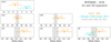 |
Fig. 4. WFI2033−4723 time-delay estimates using the WFI data set with the A1 and A2 light curves separated. The A1A2 and BC measurements from Morgan et al. (2018) are reported for comparison. We also report the “PyCS-mult” estimates from Fig. 3, obtained using the virtual A light curve, represented in this figure as shaded vertical bands. In this latter case, we report the AB and AC time-delay estimates in the A1B/A2B and A1C/A2C panels, respectively. We note that the BC estimate from WFI presented here slightly differs from Fig. 3 since the free-knot spline estimates used in the combined group are obtained by a joint fit to all of the light curves, and so are sensitive to the use of A1 and A2 instead of A. The values above each measurement give the 50th, 16th and 84th percentiles of the respective probability distributions. |
For the WFI data set, we find a marginal evidence for the A2 light curve to lead A1, whereas Morgan et al. (2018) find the opposite. We note that basic lens mass models explored in Vuissoz et al. (2008) predict 1 < ΔtA1A2 < 3, with A1 leading A2. The other delays are very close to the WFI ones obtained with A = A1 + A2 – yet with worse precision and thus consistent with “PyCS-mult” results assuming a zero delay between A1 and A2. Despite the worse precision, using A1B and A2B (or A1C and A2C) in the lens models has the advantage over using AB (or AC) of providing an extra constraint in the form of an independent time-delay estimate. It also solves the issue of the anchoring position of the A = A1 + A2 virtual image; when assuming a given cosmology and predicting the time-delay surface, one sees that the latter does not behave linearly with respect to the images position (G.C.-F. Chen, private communication). In other words, the mean position between the A1 and A2 images does not predict an excess of time delay being the mean of the individual A1 and A2 excesses of time delay. Consequently, allocating time delays to each of the A1 and A2 images prevents a potential bias in the lens models.
3.4. Robustness tests
To complete our analysis of the time delays of WFI2033−4723, we conduct a number of robustness tests to ensure the validity of our results (Sect. 3.2, hereafter the fiducial results).
The first test focuses on the Group combination threshold σthresh that was fixed at 0.5. Recall that this parameter controls how the Groups of time-delay estimates in a given Series (obtained by varying the estimator and generative model parameters of a given curve-shifting technique applied to a given data set) are combined. For this robustness test we examine two extreme behaviours; σthresh = 0 and σthresh ∼ ∞. For σthresh = 0, all the Groups in the series are combined, as in a proper marginalisation. For σthresh ∼ ∞, only the most precise Group is used, in a similar behaviour to the previous COSMOGRAIL publications. These two cases represent the two ends of the spectrum of plausible combinations, none of which being optimal. On the one hand, marginalising over all the Groups in the Series includes Groups whose curve-shifting technique parameters are not necessarily well-suited to represent the data; on the other hand, considering only the most precise Group increases the risk of being affected by a systematic error linked to the specific choice of curve-shifting technique parameters. Ensuring that the results obtained in both cases are in agreement with our fiducial results is a good test of the consistency of the latter. The results obtained are presented in Fig. 5. They are in very good agreement with the fiducial results, considering both precision and accuracy. This also indicates that the different Groups in each Series were already in good agreement with each other prior to the marginalisation.
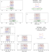 |
Fig. 5. Results of the robustness tests for WFI2033−4723 time-delay measurements presented in Sect. 3.4. The shaded vertical bands correspond to our fiducial results, labelled “PyCS-mult” and “PyCS – WFI” in Figs. 3 and 4 for the top and bottom groups of panels, respectively. The values indicated above each measurement represent the 50th, 10th and 840th percentiles of the respective probability distributions. |
The second test focuses on the generative model, especially on the way the noise in the mock data is generated. Currently, as described in Sect. 3.1, it is a combination of white and red noise whose parameters are manually adjusted on a subset of mock light curves, until the statistical properties of the fit residuals match the ones computed on the real data (see Tewes et al. 2013a, for details). The noise parameters to adjust differ for each choice of data set and generative models parameters; in total, the present work required the adjustment of 36 sets of noise parameters. Although tedious, this procedure remains tractable when analysing a single lens system. However, it does not scale well for the analysis of a large collection of systems. For this reason, we developed a new, completely automated generative model that is based on the power spectrum of the data residuals to generate the noise in the mock curves. In brief, this new model computes the power spectrum of the residuals of the spline fit via Fourier transform. In Fourier space, the phases of the signal are randomized while the amplitudes are kept the same, and the signal is then reversed to real space via inverse Fourier transform. This process allows one to generate a mock realisation of the residuals which respect the statistical properties of the data residuals. This mock noise is then added on top of the intrinsic and extrinsic variability models obtained using free-knot splines fit on the real data, similarly to what is descibed in Sect. 3.1. A more detailed description of this new generative model will be presented in a forthcoming work (Millon et al., in prep.). The results of this new generative model are presented in Fig. 5 and are labelled “PS Noise”. They use the same estimator and generative model parameters as our fiducial model presented in Table 2, and are in excellent agreement with the fiducial results. This test assesses the robustness of our fiducial noise generation scheme, but also highlights the performance of the new scheme. We thus decide to use the new scheme for the remaining robustness tests presented in this section since it is much easier to apply than the fiducial one.
Finally, for the analysis of the previous H0LiCOW lenses we used a different framework to measure time delays in which all the data sets were combined into a single set of light curves. Although in the current framework we have good reasons to separately analyse the data sets, we want to assess the effect of merging the data sets on the final time-delay estimates. This provides an important insight on the robustness of the previous time-delay measurements used by the H0LiCOW collaboration (see Tewes et al. 2013b for RXJ1131−1231 and Bonvin et al. 2017 for HE 0435−1223 – an updated measurement of the time delays of these two systems will be presented in Millon et al., in prep.). We merge the data sets by applying an offset in magnitude that is computed by minimizing the scatter between overlapping parts of each light curve and each data set. We explore two combinations, one with the four data sets combined and one without the WFI data set; since the latter stands out the most in terms of signal-to-noise ratio, sampling and duration, we want to assess its weight in the final combination. The results are presented in the upper panel of Fig. 5. We can see that the addition of the WFI data set has a clear impact, shifting the combined results towards the delays obtained on the WFI data set alone and significantly improving the overall precision. It is however less precise than our fiducial results.
4. Microlensing time delay
In this section, we compute the impact of the microlensing time delay, a speculative effect first described in Tie & Kochanek (2018) that we summarize below. The analysis performed in this section is similar to the one presented in Bonvin et al. (2018) for the lensed quasar PG1115+080, itself based on the original work of Tie & Kochanek (2018). In the following, we use the terminology introduced in Bonvin et al. (2019).
If it were possible to observe the lensed images with a resolution of a few microarcseconds, the spatial profile of the source would reveal the accretion disk of the quasar. One possible model characterisation of the accretion disk emission is the lamp-post model (e.g. Cackett et al. 2007; Starkey et al. 2016), that predicts a temperature change propagating across the disk driven by temperature variations at the center, thus triggering radiation. As a result, the emission from the outer regions of the disk follow the emission from the inner regions, but with a delay. As the disk is seen as a point source at the spatial resolution we are working with, the observed light curves are a blend of the light emitted from all the spatial regions of the source visible through the chosen filter. Due to the delayed emission in the outer regions, the variations of the observed, blended light curves are seen slightly delayed with respect to the variations of hypothetical, unblended light curves of the disk’s inner regions. This excess of time delay associated to the lamp-post model of variability is called geometrical time delay, as it relates to the spatial extension of the source. Since the geometrical delay is the same in all lensed images, it cancels out when measuring the delay between two images, and has no impact on the cosmological time delay measurement, which is the delay of interest for time-delay cosmography.
However, stars and/or other compact objects in the lens galaxy act as microlenses and differentially magnify the various regions of the lensed accretion disk. The net effect of this micromagnification is to reweight the geometrical delay for each lensed image; the additional excess of time delay introduced by the reweighting is called the microlensing time delay. Since the position of the microlenses in the lens galaxy is random, the excesses of microlensing time delays are uncorrelated and so do not cancel out between images. This results in a bias when measuring cosmological time delays between two lensed images.
In order to quantify the contribution of the microlensing time delay on the measured time delays, we first simulate microlensing magnification maps at the image positions, using the lens model from H0LiCOW XII (see Table B1). The convergence, shear and stellar mass fraction used to generate the microlensing maps are given in Table 3.
κ, γ, and κ⋆/κ at each lensed image position from the macro model presented in H0LiCOW XII.
We use GPU-D (Vernardos et al. 2014), a GPU-accelerated implementation of the inverse ray-shooting technique from Wambsganss et al. (1992)3 that produces a magnification map in the source plane from a spatially random distribution of microlenses in the lens plane. We assume that the microlenses follow a Salpeter mass function with a ratio of the upper to lower masses of r = 100 and a mean microlens mass of ⟨M⟩=0.3 M⊙4. Each map has 8192 × 8192 pixels, representing a physical size of 20 Einstein radii ⟨REin⟩, defined as:
where Dd, Ds and Dds are the angular diameter distances5 between the observer and the deflector (i.e. the lens galaxy), the observer and the source and the deflector and the source, respectively. A 20⟨REin⟩ square region is sufficiently large to statistically sample the effects of microlensing. We do not present in this work what these magnification maps look like, but the interested reader can have a look at Fig. 2 of Bonvin et al. (2019) for an example.
The quasar accretion disk is modelled using the thin-disk model of Shakura & Sunyaev (1973). The thin-disk model requires (i) the wavelength at which the observations are made, that we take as the center of the WFI BB#Rc/162 filter (6517.25 Å)6, (ii) an Eddington luminosity ratio L/LE fixed at 0.3, (iii) a radiative efficiency for the black hole at the center of the accretion disk of η = 0.1 and (iv) a black hole mass of MBH = 4.26 × 10⁸ M⊙ taken from Sluse et al. (2012). This gives an estimated disk radius of R0 = 1.291 × 1015 cm. Our choices of L/LE, η and MBH follow Morgan et al. (2018), but other values for these parameters are possible. For example, Motta et al. (2017) estimate a black-hole mass of MBH = 1.2 × 10⁸ M⊙, albeit with a much larger uncertainty, based on microlensing estimates of the accretion disk size. Adopting this value will greatly reduce the predicted size of the accretion disk, and consequently the predicted microlensing time delay by a factor of ∼2.3. We however decide to use the Sluse et al. (2012) black-hole mass estimate since it is based on the more standard virial mass estimates using observations of the MgII emission lines.
Next, we place the disk at a specific position on the magnification maps. One can compute the excess of microlensing time delay by reweighting the excess of geometrical time delay across the disk by the microlensing magnification. Integrating over all the pixels of the disk, we obtain the excess of microlensing time delay (see Eq. (10) in Tie & Kochanek 2018). By marginalizing over all the possible source positions in the microlensing maps, we obtain probability distributions for the excess of microlensing time delay for each lensed images. These are presented in Fig. 6. We also explore two extra configurations of the thin-disk model where we multiply the theoretical characteristic radius R0 by a factor of two and three. This is motivated by the fact that direct estimates of disk sizes using either microlensing (e.g. Rojas et al. 2014; Jiménez-Vicente et al. 2015; Morgan et al. 2018) and also reverberation mapping (e.g. Shappee et al. 2014; Edelson et al. 2015; Lira et al. 2015; Fausnaugh et al. 2016) generally infer sizes 2–3 times larger than the thin-disk theory predictions. The black-hole mass versus source size relation fitted on the analysis of the modeled microlensing of 14 lensed quasars in Morgan et al. (2018) predicts a source size ∼three times larger than the thin-disk model prediction, which corresponds to the higher value we explore here. We keep the disc inclination and position angle at zero across all our tests, as varying these produces only a second-order effect on the amplitude of the excess of microlensing time delay (e.g Tie & Kochanek 2018; Bonvin et al. 2018).
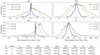 |
Fig. 6. Distributions of the excess of microlensing time delay for the four lensed image of WFI2033−4723. The values displayed represent the 16th, 50th and 84th percentiles of the plotted distributions. The thicker lines (in blue) indicate the fiducial case where the source size corresponds to the thin-disk model prediction. The vertical dashed grey lines represent the case where no microlensing time-delay is present. The table below the figure reports the percentiles of the distributions of the combined image A as well as the lensed image pair. |
A proper inclusion of the microlensing time delay into the cosmological analysis should be done cautiously. The distributions and values presented in Fig. 6 are computed assuming a source position fixed in the microlensing map. However, due to the transverse motion of the source behind the lens galaxy, microlensing time delay changes over time. As highlighted in Bonvin et al. (2019), what drives the effect of microlensing time delay is not the absolute amount of micromagnification, but the spatial variability of the micromagnification across the source profile. Thus, the time it takes for the source to fully cross a critical curve in the magnification map is a characteristic of the period over which one can expect the microlensing time delay to potentially strongly affect the time delay measurements (see e.g. Mosquera & Kochanek 2011, for estimates of typical time-scales).
A conservative approach to include microlensing time delay in our measurements is to simply convolve the probability distributions presented in the table of Fig. 6 with the time-delay measurement uncertainties presented in Sect. 3.2. A more sophisticated approach has been proposed in Chen et al. (2018a), that takes into account the discrepancies between the measured time-delays and the models predictions. However, there is presently no formalism that takes into account the duration of the monitoring campaign. In the case of WFI2033−4723, we follow the approach from Chen et al. (2018a). This analysis is presented in H0LiCOW XII, where the results with a source size of 1R0 have been included by default. H0LiCOW XII also shows that including or ignoring microlensing time-delay has a minimal impact on the time-delay distance inference for WFI2033−4723. As a final remark, we note that our measured A1-A2 delay from the WFI data set is consistent with zero, as predicted by the macro lens model; although not incompatible with the existence of microlensing time delay, it does not favor large source sizes.
5. Conclusions
This work is part of a series carrying out a new analysis of quadruply lensed system WFI2033−4723 for time-delay cosmography. H0LiCOW X studies the environment of the lens galaxy and H0LiCOW XII models the lens system. This work focuses on the measurement of the time delays between the multiple images of the lensed source. The key points are summarised as follows:
-
We present the most complete collection of monitoring data of WFI2033−4723 to date. It totals ∼450 h of monitoring, divided over four data sets (WFI, ECAM, C2 and SMARTS) from four different instruments and spanning more than 14 years of observations. It notably includes a full season of high-cadence (daily) and high-precision (millimagnitude) monitoring with the WFI instrument mounted on the MPIA 2.2 m telescope at La Silla Observatory. The monitoring data are turned into light curves using a pipeline built around the MCS deconvolution algorithm (Magain et al. 1998; Cantale et al. 2016), allowing us to accurately deblend the light from the lensed quasar images even in poor seeing conditions.
-
The time delays are estimated individually for each data set using the open-source PyCS software (Tewes et al. 2013a; Bonvin et al. 2016). The measurements from each data set are mutually consistent. We choose to combine them into a single group of time-delay estimates, resulting in
 (2.1% precision),
  (5.6%) and
  (2.2%) days.
 -
The higher signal-to-noise ratio and better seeing of the WFI exposures allows us to separate the A1 and A2 images of the lensed quasar into two light curves. The time-delay measurement between the two images yields
 days, consistent with a null delay.
 -
Unlike the time-delay estimates used in the past by H0LiCOW, the estimates presented in this work are obtained by marginalizing over the various parameters of our curve-shifting techniques following the formalism introduced in Bonvin et al. (2018). In addition, a series of tests are conducted to ensure the robustness of our results. Updating the time-delay estimates of the other H0LiCOW lens systems is planned for a future milestone update.
-
We estimate the contribution of the microlensing time delay to the measured delays using the quasar black-hole mass estimate from Sluse et al. (2012). The predictions obtained using the standard thin-disk model are moderate, and are implemented by default at the lens modelling stage (H0LiCOW XII). Increasing the disk size to match the measurements from microlensing studies (Morgan et al. 2018) increases the contribution of microlensing time delay. The precision of the measured time delays neither confirms nor rules out the presence of microlensing time delay in the data.
The measured time delays and estimated microlensing time delays are used at the lens modelling stage (H0LiCOW XII) to measure the time-delay distance of WFI2033−4723 and infer a value of the Hubble constant H0. H0LiCOW XIII combines the time-delay distance of WFI2033−4723 with two other lenses systems fully analysed by H0LiCOW (B1608+656 from Suyu et al. 2010 and SDSS 1206+4332 from Birrer et al. 2019) with a combined analysis of HST+AO images of RXJ1131−1231, HE 0435−1223 and PG1115+080 from a joint STRIDES+H0LiCOW effort (Chen et al. 2019), turning them into the most precise joint inference of H0 from time-delay cosmography to date. It also updates the joint inference with other cosmological probes, superseding the previous results of H0LiCOW V (Bonvin et al. 2017).
This paper is the third of a series reporting successful COSMOGRAIL monitoring campaigns with the MPIA 2.2 m telescope; it follows the time-delay measurements for DES J0408−5354 (Courbin et al. 2018) and PG1115+080 (Bonvin et al. 2018). Significantly improving the precision with which the Hubble constant can be determined from time-delay cosmography will require the analysis of dozens of lensed systems. Being able to measure robust time-delay estimates in a short amount of time is crucial in this regard. Our goal is to measure several tens of new delays in the next 5 years. Prospects are excellent, as the precision of the time delays for individual objects is of the order of 2–5% in only 1 season of high-cadence (daily) and high SNR (> 500 per quasar image) monitoring for each object. With smaller telescopes (1 m) and lower cadence (1 point every 4 days) such a precision typically required 10 years of effort per object.
Technically speaking, Wambsganss et al. (1992) use a tree code to simplify the computations whereas (Vernardos et al. 2014) do the full computation.
We note that Poindexter & Kochanek (2010) showed that a Salpeter mass function might not a good model for microlenses, but in the present application replacing it with a Chabrier or uniform mass function does not produce significant differences in the microlensing time-delay distributions.
Acknowledgments
COSMOGRAIL and H0LiCOW are made possible thanks to the continuous work of all observers and technical staff obtaining the monitoring observations, in particular at the Swiss Euler telescope at La Silla Observatory. We also warmly thank R. Gredel, H.-W. Rix and T. Henning for allowing us to observe with the MPIA 2.2 m telescope and for ensuring the daily cadence of the observations is achieved. We thank the anonymous referee for his/her careful reading and meaningful comments on this manuscript. This research is support by the Swiss National Science Foundation (SNSF) and by the European Research Council (ERC) under the European Union’s Horizon 2020 research and innovation programme (COSMICLENS: grant agreement No 787866). D.S. acknowledges funding support from a Back to Belgium grant from the Belgian Federal Science Policy (BELSPO). S.H.S. and D.C.-Y.C. thank the Max Planck Society for support through the Max Planck Research Group for SHS. This work was supported by World Premier International Research Center Initiative (WPI Initiative), MEXT, Japan. K.C.W. is supported in part by an EACOA Fellowship awarded by the East Asia Core Observatories Association, which consists of the Academia Sinica Institute of Astronomy and Astrophysics, the National Astronomical Observatory of Japan, the National Astronomical Observatories of the Chinese Academy of Sciences, and the Korea Astronomy and Space Science Institute. C.D.F. acknowledges support for this work from the National Science Foundation under Grant No. AST-1715611. P.J.M. acknowledges support from the US Department of Energy under contract number DE-AC02-76SF00515. T.T. thanks the Packard Foundation for generous support through a Packard Research Fellowship, the NSF for funding through NSF grant AST-1450141, “Collaborative Research: Accurate cosmology with strong gravitational lens time delays”. T. A. acknowledges support by the Ministry for the Economy, Development, and Tourism’s Programa Inicativa Científica Milenio through grant IC 12009, awarded to The Millennium Institute of Astrophysics (MAS). C.S.K is supported by NSF grants AST-1515876, AST-1515927 and AST-181440 as well as a fellowship from the Radcliffe Institute for Advanced Study at Harvard University. C.M is supported by the NSF grant #1614018. V.M. acknowledges the support from Centro de Astrofísica de Valparaíso. This research made use of Astropy, a community-developed core Python package for Astronomy (Astropy Collaboration 2013, 2018), the 2D graphics environment Matplotlib (Hunter 2007) and the source extraction software Sextractor (Bertin & Arnouts 1996).
References
- Abbott, B. P., Abbott, R., Abbott, T. D., et al. 2017, Nature, 551, 85 [NASA ADS] [CrossRef] [PubMed] [Google Scholar]
- Amendola, L., Dirian, Y., Nersisyan, H., & Park, S. 2019, JCAP, 2019, 045 [CrossRef] [Google Scholar]
- Astropy Collaboration (Robitaille, T. P., et al.) 2013, A&A, 558, A33 [NASA ADS] [CrossRef] [EDP Sciences] [Google Scholar]
- Astropy Collaboration (Price-Whelan, A. M., et al.) 2018, AJ, 156, 123 [Google Scholar]
- Bautista, J. E., Busca, N. G., Guy, J., et al. 2017, A&A, 603, A12 [NASA ADS] [CrossRef] [EDP Sciences] [Google Scholar]
- Bertin, E., & Arnouts, S. 1996, A&AS, 117, 393 [NASA ADS] [CrossRef] [EDP Sciences] [Google Scholar]
- Birrer, S., Treu, T., Rusu, C. E., et al. 2019, MNRAS, 484, 4726 [NASA ADS] [CrossRef] [Google Scholar]
- Bonvin, V., Tewes, M., Courbin, F., et al. 2016, A&A, 585, A88 [NASA ADS] [CrossRef] [EDP Sciences] [Google Scholar]
- Bonvin, V., Courbin, F., Suyu, S. H., et al. 2017, MNRAS, 465, 4914 [NASA ADS] [CrossRef] [Google Scholar]
- Bonvin, V., Chan, J. H. H., Millon, M., et al. 2018, A&A, 616, A183 [NASA ADS] [CrossRef] [EDP Sciences] [Google Scholar]
- Bonvin, V., Tihhonova, O., Millon, M., et al. 2019, A&A, 621, A55 [NASA ADS] [CrossRef] [EDP Sciences] [Google Scholar]
- Braatz, J., Pesce, D., Condon, J., & Reid, M. 2018, in Science with a Next Generation Very Large Array, ed. E. Murphy, ASP Conf. Ser., 517, 821 [NASA ADS] [Google Scholar]
- Cackett, E. M., Horne, K., & Winkler, H. 2007, MNRAS, 380, 669 [NASA ADS] [CrossRef] [Google Scholar]
- Cantale, N., Courbin, F., Tewes, M., Jablonka, P., & Meylan, G. 2016, A&A, 589, A81 [NASA ADS] [CrossRef] [EDP Sciences] [Google Scholar]
- Cao, S., Zheng, X., Biesiada, M., et al. 2017, A&A, 606, A15 [NASA ADS] [CrossRef] [EDP Sciences] [Google Scholar]
- Capozziello, S., Ruchika, K., & Sen, A. A. 2019, MNRAS, 484, 4484 [NASA ADS] [CrossRef] [Google Scholar]
- Chen, G. C.-F., Chan, J. H. H., Bonvin, V., et al. 2018a, MNRAS, 481, 1115 [NASA ADS] [CrossRef] [Google Scholar]
- Chen, H.-Y., Fishbach, M., & Holz, D. E. 2018b, Nature, 562, 545 [NASA ADS] [CrossRef] [Google Scholar]
- Chen, G. C. F., Fassnacht, C. D., Suyu, S. H., et al. 2019, ArXiv e-prints [arXiv: 1907.02533] [Google Scholar]
- Courbin, F., Bonvin, V., Buckley-Geer, E., et al. 2018, A&A, 609, A71 [NASA ADS] [CrossRef] [EDP Sciences] [Google Scholar]
- DES Collaboration (Abbott, T. M. C., et al.) 2018, MNRAS, 480, 3879 [NASA ADS] [CrossRef] [Google Scholar]
- Dhawan, S., Jha, S. W., & Leibundgut, B. 2018, A&A, 609, A72 [NASA ADS] [CrossRef] [EDP Sciences] [Google Scholar]
- Edelson, R., Gelbord, J. M., Horne, K., et al. 2015, ApJ, 806, 129 [NASA ADS] [CrossRef] [Google Scholar]
- Fausnaugh, M. M., Denney, K. D., Barth, A. J., et al. 2016, ApJ, 821, 56 [NASA ADS] [CrossRef] [Google Scholar]
- Feeney, S. M., Peiris, H. V., Williamson, A. R., et al. 2019, Phys. Rev. Lett., 122, 061105 [NASA ADS] [CrossRef] [Google Scholar]
- Giannini, E., Schmidt, R. W., Wambsganss, J., et al. 2017, A&A, 597, A49 [NASA ADS] [CrossRef] [EDP Sciences] [Google Scholar]
- Hikage, C., Oguri, M., Hamana, T., et al. 2019, PASJ, 71, 43 [NASA ADS] [CrossRef] [Google Scholar]
- Hunter, J. D. 2007, Comput. Sci. Eng., 9, 90 [NASA ADS] [CrossRef] [Google Scholar]
- Jang, I. S., Hatt, D., Beaton, R. L., et al. 2018, ApJ, 852, 60 [NASA ADS] [CrossRef] [Google Scholar]
- Jiménez-Vicente, J., Mediavilla, E., Kochanek, C. S., & Muñoz, J. A. 2015, ApJ, 806, 251 [NASA ADS] [CrossRef] [Google Scholar]
- Kasliwal, V. P., Vogeley, M. S., & Richards, G. T. 2015, MNRAS, 451, 4328 [NASA ADS] [CrossRef] [Google Scholar]
- Köhlinger, F., Viola, M., Joachimi, B., et al. 2017, MNRAS, 471, 4412 [NASA ADS] [CrossRef] [Google Scholar]
- Kozłowski, S., Kochanek, C. S., Udalski, A., et al. 2010, ApJ, 708, 927 [NASA ADS] [CrossRef] [Google Scholar]
- Kozmanyan, A., Bourdin, H., Mazzotta, P., Rasia, E., & Sereno, M. 2019, A&A, 621, A34 [NASA ADS] [CrossRef] [EDP Sciences] [Google Scholar]
- Lira, P., Arévalo, P., Uttley, P., McHardy, I. M. M., & Videla, L. 2015, MNRAS, 454, 368 [NASA ADS] [CrossRef] [Google Scholar]
- Magain, P., Courbin, F., & Sohy, S. 1998, ApJ, 494, 472 [NASA ADS] [CrossRef] [Google Scholar]
- Marshall, P., Rajguru, N., & Slosar, A. 2006, Phys. Rev. D, 73, 067302 [NASA ADS] [CrossRef] [Google Scholar]
- Molinari, N., Durand, J., & Sabatier, R. 2004, Comput. Stat. Data Anal., 45, 159 [CrossRef] [Google Scholar]
- Morgan, N. D., Caldwell, J. A. R., Schechter, P. L., et al. 2004, AJ, 127, 2617 [NASA ADS] [CrossRef] [Google Scholar]
- Morgan, C. W., Hyer, G. E., Bonvin, V., et al. 2018, ApJ, 869, 106 [Google Scholar]
- Mörtsell, E., & Dhawan, S. 2018, JCAP, 9, 025 [CrossRef] [Google Scholar]
- Mosquera, A. M., & Kochanek, C. S. 2011, ApJ, 738, 96 [NASA ADS] [CrossRef] [Google Scholar]
- Motta, V., Mediavilla, E., Rojas, K., et al. 2017, ApJ, 835, 132 [NASA ADS] [CrossRef] [Google Scholar]
- Mushotzky, R. F., Edelson, R., Baumgartner, W., & Gandhi, P. 2011, ApJ, 743, L12 [NASA ADS] [CrossRef] [Google Scholar]
- Pandey, K. L., Karwal, T., & Das, S. 2019, ArXiv e-prints [arXiv:1902.10636] [Google Scholar]
- Planck Collaboration I. 2018, A&A, submitted [arXiv:1807.06205] [Google Scholar]
- Planck Collaboration VI. 2018, A&A, submitted [arXiv:1807.06209] [Google Scholar]
- Poindexter, S., & Kochanek, C. S. 2010, ApJ, 712, 658 [NASA ADS] [CrossRef] [Google Scholar]
- Poulin, V., Smith, T. L., Karwal, T., & Kamionkowski, M. 2019, Phys. Rev. L, 122, 221301 [Google Scholar]
- Refsdal, S. 1964, MNRAS, 128, 307 [NASA ADS] [CrossRef] [Google Scholar]
- Reid, M. J., Braatz, J. A., Condon, J. J., et al. 2013, ApJ, 767, 154 [NASA ADS] [CrossRef] [Google Scholar]
- Riess, A. G., Casertano, S., Yuan, W., Macri, L. M., & Scolnic, D. 2019, ApJ, 876, 85 [NASA ADS] [CrossRef] [Google Scholar]
- Rojas, K., Motta, V., Mediavilla, E., et al. 2014, ApJ, 797, 61 [NASA ADS] [CrossRef] [Google Scholar]
- Rusu, C. E., Fassnacht, C. D., Sluse, D., et al. 2017, MNRAS, 467, 4220 [NASA ADS] [CrossRef] [Google Scholar]
- Rusu, C. E., Wong, K. C., Bonvin, V., et al. 2019, MNRAS, submitted [arXiv:1905.09338] [Google Scholar]
- Shakura, N. I., & Sunyaev, R. A. 1973, A&A, 24, 337 [NASA ADS] [Google Scholar]
- Shappee, B. J., Prieto, J. L., Grupe, D., et al. 2014, ApJ, 788, 48 [NASA ADS] [CrossRef] [Google Scholar]
- Sluse, D., Hutsemékers, D., Courbin, F., Meylan, G., & Wambsganss, J. 2012, A&A, 544, A62 [NASA ADS] [CrossRef] [EDP Sciences] [Google Scholar]
- Sluse, D., Sonnenfeld, A., Rumbaugh, N., et al. 2017, MNRAS, 470, 4838 [NASA ADS] [CrossRef] [Google Scholar]
- Sluse, D., Rusu, C. E., Fassnacht, C. D., et al. 2019, MNRAS, submitted [arXiv:1905.08800] [Google Scholar]
- Starkey, D. A., Horne, K., & Villforth, C. 2016, MNRAS, 456, 1960 [NASA ADS] [CrossRef] [Google Scholar]
- Suyu, S. H., Marshall, P. J., Auger, M. W., et al. 2010, ApJ, 711, 201 [NASA ADS] [CrossRef] [Google Scholar]
- Suyu, S. H., Treu, T., Hilbert, S., et al. 2014, ApJ, 788, L35 [NASA ADS] [CrossRef] [Google Scholar]
- Suyu, S. H., Bonvin, V., Courbin, F., et al. 2017, MNRAS, 468, 2590 [Google Scholar]
- Suyu, S. H., Chang, T.-C., Courbin, F., & Okumura, T. 2018, Space Sci. Rev., 214, 91 [NASA ADS] [CrossRef] [Google Scholar]
- Tewes, M., Courbin, F., & Meylan, G. 2013a, A&A, 553, A120 [NASA ADS] [CrossRef] [EDP Sciences] [Google Scholar]
- Tewes, M., Courbin, F., Meylan, G., et al. 2013b, A&A, 556, A22 [NASA ADS] [CrossRef] [EDP Sciences] [Google Scholar]
- Tie, S. S., & Kochanek, C. S. 2018, MNRAS, 473, 80 [NASA ADS] [CrossRef] [Google Scholar]
- Tihhonova, O., Courbin, F., Harvey, D., et al. 2018, MNRAS, 477, 5657 [NASA ADS] [CrossRef] [Google Scholar]
- Treu, T., & Marshall, P. J. 2016, A&ARv, 24, 11 [Google Scholar]
- Troxel, M. A., Krause, E., Chang, C., et al. 2018, MNRAS, 479, 4998 [NASA ADS] [CrossRef] [Google Scholar]
- Vernardos, G., Fluke, C. J., Bate, N. F., & Croton, D. 2014, ApJS, 211, 16 [NASA ADS] [CrossRef] [Google Scholar]
- Vuissoz, C., Courbin, F., Sluse, D., et al. 2008, A&A, 488, 481 [NASA ADS] [CrossRef] [EDP Sciences] [Google Scholar]
- Wambsganss, J., Witt, H. J., & Schneider, P. 1992, A&A, 258, 591 [NASA ADS] [Google Scholar]
- Wong, K. C., Suyu, S. H., Auger, M. W., et al. 2017, MNRAS, 465, 4895 [NASA ADS] [CrossRef] [Google Scholar]
- Wong, K. C., Suyu, S. H., Chen, G. C.-F., et al. 2019, MNRAS submitted, [arXiv: 1907.04869] [Google Scholar]
- Zu, Y., Kochanek, C. S., Kozłowski, S., & Udalski, A. 2013, ApJ, 765, 106 [NASA ADS] [CrossRef] [Google Scholar]
All Tables
κ, γ, and κ⋆/κ at each lensed image position from the macro model presented in H0LiCOW XII.
All Figures
|
Fig. 1. Part of the field of view of WFI2033−4723 seen through the WFI instrument at the 2.2 m MPIA telescope. The field is a stack of 312 images with seeing ≤1″.4 and ellipticity ≤0.18, totalling ∼28 h of exposure. The insert represent a single, 320 s exposure of the lens in |
| In the text | |
|
Fig. 2. WFI2033−4723 light curves from the four different instruments used in this work. Top panel: Euler data sets (C2+ECAM instruments), with the change occuring in October 2010, corresponding to the small gap visible in the 2010 season. Middle panel: SMARTS data set. Bottom left panel: WFI data set, where the A1 and A2 images were individually resolved thanks to superior image quality and longer exposure times. We note that different calibration stars were used for the different data sets, hence the differences in the relative magnitudes between the instruments. Bottom right panel: normalised distribution of the airmass and seeing of all the individual exposures in each data set. |
| In the text | |
|
Fig. 3. WFI2033−4723 time-delay estimates. The colored points labelled “PyCS” represent the final time-delay estimates for each data set, obtained after combining the curve-shifting technique parameters following the marginalisation scheme presented in Sect. 3.1. The gray and black points, respectively labelled “PyCS-sum” and “PyCS-mult” represent the marginalisation and combination of the results obtained from the individual data sets. Indicated with small diamonds and dashed lines are the AB and BC delays taken from Morgan et al. (2018) and Vuissoz et al. (2008), respectively. The similar color between “PyCS -C2” and Vuissoz 2008 indicates that both measurement share the same data set, although less complete in the latter case (see Table 1). The values indicated above each measurement represent the 50th, 16th and 84th percentiles of the respective probability distributions. |
| In the text | |
|
Fig. 4. WFI2033−4723 time-delay estimates using the WFI data set with the A1 and A2 light curves separated. The A1A2 and BC measurements from Morgan et al. (2018) are reported for comparison. We also report the “PyCS-mult” estimates from Fig. 3, obtained using the virtual A light curve, represented in this figure as shaded vertical bands. In this latter case, we report the AB and AC time-delay estimates in the A1B/A2B and A1C/A2C panels, respectively. We note that the BC estimate from WFI presented here slightly differs from Fig. 3 since the free-knot spline estimates used in the combined group are obtained by a joint fit to all of the light curves, and so are sensitive to the use of A1 and A2 instead of A. The values above each measurement give the 50th, 16th and 84th percentiles of the respective probability distributions. |
| In the text | |
|
Fig. 5. Results of the robustness tests for WFI2033−4723 time-delay measurements presented in Sect. 3.4. The shaded vertical bands correspond to our fiducial results, labelled “PyCS-mult” and “PyCS – WFI” in Figs. 3 and 4 for the top and bottom groups of panels, respectively. The values indicated above each measurement represent the 50th, 10th and 840th percentiles of the respective probability distributions. |
| In the text | |
|
Fig. 6. Distributions of the excess of microlensing time delay for the four lensed image of WFI2033−4723. The values displayed represent the 16th, 50th and 84th percentiles of the plotted distributions. The thicker lines (in blue) indicate the fiducial case where the source size corresponds to the thin-disk model prediction. The vertical dashed grey lines represent the case where no microlensing time-delay is present. The table below the figure reports the percentiles of the distributions of the combined image A as well as the lensed image pair. |
| In the text | |
Current usage metrics show cumulative count of Article Views (full-text article views including HTML views, PDF and ePub downloads, according to the available data) and Abstracts Views on Vision4Press platform.
Data correspond to usage on the plateform after 2015. The current usage metrics is available 48-96 hours after online publication and is updated daily on week days.
Initial download of the metrics may take a while.