| Issue |
A&A
Volume 629, September 2019
|
|
|---|---|---|
| Article Number | A121 | |
| Number of page(s) | 16 | |
| Section | Planets and planetary systems | |
| DOI | https://doi.org/10.1051/0004-6361/201935542 | |
| Published online | 17 September 2019 | |
Near-infrared polarimetric study of near-Earth object 252P/LINEAR: an implication of scattered light from the evolved dust particles
1
Department of Physics and Astronomy, Seoul National University,
1 Gwanak,
Seoul 08826,
Republic of Korea
e-mail: ishiguro@astro.snu.ac.kr
2
Department of Astronomy, Graduate School of Science, The University of Tokyo,
7-3-1 Hongo, Bunkyo-ku,
Tokyo 113-0033,
Japan
3
Okayama Observatory, Kyoto University,
3037-5 Honjo,
Kamogata, Asakuchi,
Okayama 719-0232,
Japan
4
National Astronomical Observatory of Japan,
2-21-1 Osawa,
Mitaka,
Tokyo 181-8588,
Japan
5
Astrobiology Center,
2-21-1 Osawa,
Mitaka,
Tokyo 181-8588,
Japan
6
Faculty of Science, Kagoshima University,
21-24 Korimoto,
Kagoshima,
Kagoshima 890-8580,
Japan
7
Department of Physics, Tokyo Institute of Technology,
Meguro,
Tokyo 152-8551,
Japan
Received:
26
March
2019
Accepted:
8
July
2019
Context. Comets undergo resurfacing due to solar radiation, while their primordial interiors remain unchanged. Multi-epoch observations of comets enable us to characterize a change in sublimation pattern as a function of heliocentric distance, which in turn provides information on the dust environments of comets.
Aims. We aim to constrain the size and porosity of ejected dust particles from comet 252P/LINEAR and their evolution near perihelion via near-infrared (NIR) multiband polarimetry. A close approach of the comet to the Earth in March 2016 (~0.036 au) provided a rare opportunity for the sampling of the comet at high spatial resolution.
Methods. We made NIR JHKS-band (1.25–2.25 μm) polarimetric observations of the comet for 12 days near perihelion, interspersed between broadband optical (0.48–0.80 μm) imaging observations over four months. In addition, a dynamical simulation of the comet was performed 1000 yr backward in time.
Results. We detected two discontinuous brightness enhancements of 252P/LINEAR. Before the first enhancement, the NIR polarization degrees of the comet were far lower than those of ordinary comets at a given phase angle. Soon after the activation, however, they increased by ~13% at most, showing unusual blue polarimetric color over the J and H bands (−2.55% μm−1 on average) and bluing of the dust color in both J−H and H−KS. Throughout the event, the polarization vector was marginally aligned perpendicular to the scattering plane (i.e., θr = 4.6°–10.9°). The subsequent postperihelion reactivation of the comet lasted for approximately 1.5 months, with a factor of ~30 times pre-activation dust mass-loss rates in the RC band.
Conclusions. The marked increase in the polarization degree with blue NIR polarimetric color is reminiscent of the behavior of a fragmenting comet D/1999 S4 (LINEAR). The most plausible scenario for the observed polarimetric properties of 252P/LINEAR is an ejection of predominantly large (well within the geometrical optics regime) and compact dust particles from the desiccated surface layer. We conjecture that the more intense solar heating that the comet has received in the near-Earth orbit would cause the paucity of small fluffy dust particles around the nucleus of the comet.
Key words: comets: individual: 252P/LINEAR / polarization / meteorites, meteors, meteoroids
© ESO 2019
1 Introduction
Comets, which are among the least altered leftovers from the early solar system, have probably preserved their primitive structures inside, whereas their surfaces change from their initial states after repetitive orbital revolutions around the Sun. Solar radiation depletes near-surface volatiles and grains with high surface-to-volume ratios (Prialnik et al. 2004), while concurrent sintering effects leads to the growth of grain-to-grain contact areas and their condensation (Kossacki et al. 1994; Thomas et al. 1994; Gundlach et al. 2018). As a result, resurfacing by the inert refractory layer (called the dust mantle) makes the surface drier and more consolidated than the bulk nuclei (Biele et al. 2015; Spohn et al. 2015; Kossacki et al. 2015). The cometary dust that we observe generally originates from such a near-surface layer or bounded boulders ejected from the last apparition (Rotundi et al. 2015; Fulle et al. 2018). Conversely, fresh particles tend to be ejected from the interiors of the nuclei in rather erratic ways, for example during a sudden brightness enhancement near perihelion or outbursts (e.g., Ishiguro et al. 2010, 2016).
The polarimetry of comets is a useful diagnostic for investigating the physical properties of dust particles, such as size and porosity (Kiselev et al. 2015). In particular, polarimetric observations at near-infrared (NIR) wavelengths (1.2–2.3 μm) have been predicted to set constraints on the porosity of dust grains by covering more dust monomers (basic constitutional units of dust aggregates with ~0.1 μm radii; e.g., Kimura et al. 2006) within a single wavelength than in the optical (Kolokolova & Kimura 2010). Electromagnetic interaction between the monomers in aggregates depolarizes the light, randomizing directional information of the scattered light, so that the lower the porosity of a dust particle, the greater the depolarization as the wavelength increases. It is thus theoretically expected that NIR polarimetry would maximize the difference between the porosities ofcometary dust, showing a more distinct contrast between the evolved hardened particles and fresh likely fluffier dust particles compared to the optical polarimetry (Kolokolova & Kimura 2010). To date, a dozen comets havebeen polarimetrically observed at the NIR, with a bias toward dynamically new or long-periodic comets. Three of them were observed with multiple NIR filters (quasi-)simultaneously (i.e., comets C/1995 O1 (Hale-Bopp), 1P/Halley, and C/1975 V1 (West)); the last was the only comet observed at large phase angles of α > 70° (Kiselev et al. 2015 and references therein).
Here, we present the results of tracking the evolution of the activity of comet 252P/LINEAR (hereafter 252P) over four months in 2016, with multiband NIR imaging polarimetric and optical imaging observations. Comet 252P attracted attention due to its close approach to the Earth (~0.036 au) and its possible dynamical pairing with comet P/2016 BA14 (PanSTARRS). Additionally, 252P had been one of the weakly active comets (Ye et al. 2016a), despite its recent ejection into the near-Earth orbit (q < 1.3 au, where q denotes the perihelion distance), which led Ye et al. (2016a,b) to suggest that 252P probably has a volatile-poor origin. However, we questioned such a scenario for the comet based on the strong C2 -rich coma of 252P observed in 2016 (McKay et al. 2017); the observational evidence suggesting the existence of icy chunks near the nucleus of the comet (Li et al. 2017; Coulson et al. 2017); and an estimated elapsed time of 252P in the near-Earth orbit (~3 × 10² yr; Tancredi 2014), which could suffice for the growth of the dust mantle (~1–10 yr near the Sun; Jewitt 2002; Kwon et al. 2016).
What if the long-lasting dormancy of 252P might originate in insulation by the sturdy mantle, not in a lack of volatiles? How does the light scattered by such evolved dust particles behave in comparison with the light scattered by freshly ejected particles from the interior? Our science objective is to characterize the activity of this near-Earth comet in its 2016 apparition. The favorable observational geometry of the comet in 2016 enabled us to sample the bright short-periodic comet with a high spatial resolution using ground-based telescopes.
This paper is organized as follows. In Sect. 2 we describe the observational methods and data analyses, and in Sect. 3 we present the results. Compared with the optical imaging observations conducted over ~four months, the NIR polarimetric observations only overlap for a short period of ~two weeks before the perihelion passage, and so in Sect. 3 we present the observational results of the data both taken at preperihelion, which we discuss in Sect. 4. Finally, in Sect. 5 we present a summary. The collateral postperihelion photometric results are found in Appendix A, showing the optical colorimetric results favorable for the presence of icy particles; the results of backward dynamical simulation and discussion on the size of the comet are described in Appendices B and C, respectively.
2 Observations and data analyses
In this section, we describe the observational methods and data analyses. The journal of our observational geometry and instrument settings is shown in Table D.1.
2.1 Observations
Near-infrared imaging polarimetric observations were conducted from UT 2016 March 02 to March 15 in daily cadence using a polarimeter SIRPOL of the NIR camera SIRIUS attached to the InfraRed Survey Facility (IRSF) 1.4 m diameter telescope at the South African Astronomical Observatory (32°22′46′′ E, 20°48′39′′ S, 1798 m), Sutherland, South Africa. SIRPOL, a single-beam polarimeter of a half-wave plate (HWP) rotator with a wire grid polarizer located upstream of the SIRIUS camera at the Cassegrain focus, simultaneously provides multiband NIR wide-field polarimetry (7.7′ × 7.7′, with the image scale of 0.45′′ pixel−1) at the J (center wavelength λC = 1.25 μm), H (λC = 1.65 μm), and KS (λC = 2.25 μm) bands (Nagayama et al. 2003; Kandori et al. 2006). A microcontroller controls the HWP rotator angle by driving a stepping motor and takes images in the sequence of 0°, 45°, 22.5°, and 67.5°. Because of the unavailability of the nonsidereal tracking mode, we set the exposure time to 5–20 s so that the elongation of the comet was smaller than ~2′′. Target observations were conducted in units of 10 sets, each of which consists of exposures at four HWP angles (0°, 45°, 22.5°, and 67.5°) dithered by ~30 pixels (13.5′′, which was large enough to avoid the coma signals). We interleaved sky observations +400 pixels in the x direction and −400 pixels in the y direction (±3′) off the detector center with every 10 sets of target observations. Seeing ranged from 0.9′′ –1.8′′ and was primarily 1.2′′.
Preperihelion Johnson R-band (λC = 0.62 μm) imaging observations were obtained from UT 2016 February 13 to March 09 using the 0.4 m diameter Lee Sang Gak telescope (LSGT) at the Siding Spring Observatory (149°03′52′′ E, 31°16′24′′ S, 1165 m), New South Wales, Australia. We used the SBIG ST-10 camera, whose CCD chip has 2184 × 1472 pixels with a 6.8 μm pixel pitch. It provides an image scale of 0.48′′ with a field of view of 17.5′ × 11.8′ (Im et al. 2015). Because of the unavailability of the nonsidereal tracking mode, we set the exposure time to 5–60 s so that the elongation of the comet was smaller than ~1′′. Seeing was approximately 1.2′′.
Postperihelion simultaneous multiband imaging observations with the Sloan Digital Sky Survey (SDSS) g′ band and the Johnson-Cousins RC and IC bands (whose λC are 0.48, 0.66, and 0.80 μm, respectively) were performed from UT 2016 March 24 to June 10 using the 0.5 m diameter telescope at the Okayama Astrophysical Observatory (OAO-50; 133°35′36′′ E, 34°34′33′′ N, 360 m), Okayama, Japan. We employed the Multicolor Imaging Telescopes for the Survey and Monstrous Explosions (MITSuME) system, which consists of three 1024 × 1024 CCD chips with a 24.0 μm pixel pitch (Kotani et al. 2005). It covers the field of view of 26′ × 26′ with a pixel resolution of 1.53′′. Nonsidereal guiding was conducted so that we obtained integrations of 30–120 s, each depending on the signal-to-noise ratio (S/N) of the comet. Airmass was variable in the range 1.1′′ –5.1′′ and seeing was primarily 2.5′′.
2.2 Data analyses
The raw observational data (polarimetric and photometric) were preprocessed with standard techniques for imaging data: bias and dark subtractions, flat-fielding, frame registration, and sky subtraction in IRAF. The pixel coordinates of the images were converted into celestial coordinates using WCSTools (Mink 1997), with field stars listed in the Two Micron All-Sky Survey (2MASS) catalog (Skrutskie et al. 2006) for the IRSF data and with stars listed in the UCAC-3 catalog (Zacharias et al. 2010) for the LSGT and OAO data. Since incomplete sky subtraction can produce a spurious false degree of linear polarization (P) signals at NIR, we took special care with the background subtraction at the level of each HWP angle image. Each set of sky frames was median-combined by matching the stars with identical WCS information and was subtracted from the target images taken at the same HWP angle. If there are still remaining counts after reduction by the standard sky subtraction process, we subtracted an arbitrary constant value measured at areas of blank sky well outside the coma to make the sky count nearly zero. The resulting object images were median-combined nightly by matching the instantaneous location of the comet as the center to eliminate contaminations (e.g., noise from background stars and cosmic rays) and to improve the S/N. In this process, we used data only if the S/N of the comet in a single image is higher than three.
The P of the comet was derived by performing photometry of focused images using APPHOT in IRAF. Since the S/N of the resulting combined images (≲80) is not high enough to perform imaging polarimetry, we decided to perform aperture polarimetry. Therefore, we integrated all signals within an aperture, losing the spatial information inside. We implemented a photopolarimetric aperture of 5 pixels (2.25′′, corresponding to the projected physical distance of 82–173 km during the polarimetric observation) in radius in all bands (J, H, and KS). The Stokes I and, subsequently, Stokes Q and U were calculated using
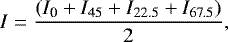 (1)
(1)

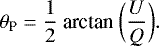
where IX denotes theintensity taken at a HWP angle of Xin degrees. The P and the polarization position angle of the strongest electric vector θP can be calculated using
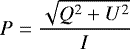 (3)
(3)
The above quantities ought to be corrected for instrumental effects, that is, for internal polarization, polarization efficiencies of each filter, and position angle offset of SIRPOL. The polarization efficiencies of the J, H, and KS filters are known to be 95.5%, 96.3%, and 98.5%, respectively, and the polarization position angle offset of the instrument is 105° in the bands (Kandori et al. 2006). For instrumental polarization (Pinst), as mentioned in detail in previous studies using SIRPOL (e.g., Kandori et al. 2006; Kwon et al. 2015) and in the recently updated results (Kusune et al. 2015), the Pinst of SIRPOL is considered negligible. Since 252P was observed at high phase angles (α = 78.8°–87.0°), where the majority of comets exhibit P ≳ 20% (Kiselev et al. 2015), an influence of Pinst on our results should be inconsequential.
Finally, the corrected P and θP were converted into quantities with respect to the scattering plane (the plane on which the Sun–comet–Earth are located) as
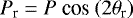 (5)
(5)
where ϕ represents the position angle of the scattering plane, the sign of which (± in Eq. (6)) was chosen to satisfy 0 ≤ (ϕ ± π/2) ≤ π (Chernova et al. 1993). Uncertainties were estimated in a standard error propagation law. We tabulated the resulting polarimetric parameters and their errors in Table 1. For polarimetric analyses, we excluded all data taken on UT 2016 March 02–03 and the data in the KS band on March 04 because of the faint comet brightness (S∕N ≲ 3) and temporal malfunction of the KS-band detector, respectively, and the data on March 05–08 because of high and fluctuating humidity conditions.
Photometric aperture sizes of the imaging (LSGT and OAO) and Stokes I (IRSF) data were all restricted to the projected physical distance of 1000 km from the center of the nucleus in radius, corresponding to 13–35 pixelsfor the LSGT data, 2–22 pixels for the OAO data, and 29–61 pixels for the IRSF data during the observing epochs. Sky brightness was subtracted by the circular annuli with widths of 5 pixels just outside the employed aperture. Flux calibration of the g′ RCIC filters was obtained from images of nearby comparison stars listed in the AAVSO Photometric All Sky Survey DR9catalog (APASS; Henden et al. 2016). We assumed a systematic error of the catalog of ~0.1 mag to take into account the calibration uncertainties (Tonry et al. 2018). SDSS magnitudes of the APASS catalog were transformed to the Johnson–Cousins magnitudes using the prescriptions for the main-sequence stars by Jester et al. (2005) and Jordi et al. (2005). In addition, we converted the IRSF magnitude system, which follows the Mauna Kea Observatories NIR filter system (Tokunaga et al. 2002), into the Johnson–Cousins RC magnitudes to know the approximate trend of the cometary activity during the IRSF observations compared to the optical data. We analyzed the Stokes I of the H-band data as a representative example, simply due to the highest S/N of the comet therein. Flux calibration of the IRSF magnitudes was obtained from the field stars of the 2MASS Point Source Catalog (Curti et al. 2003) using the conversion equations of Kato et al. (2007). The H magnitudes were then converted into the Johnson R magnitudes, assuming a solar-like spectrum of the comet for simplicity (i.e., R − H = 1.055; Binney & Merrifield 1998), and finally converted into the RC magnitudes using the prescriptions of R − RC = −0.17 (Fernie 1983). We list the apparent magnitudes of the IRSF data in Table 1.
3 Results
In this section, we report the results obtained by optical photometry and NIR polarimetry of comet 252P at its preperihelion.
3.1 Photometric results I: detection of two discontinuous activations
Figure 1 shows the temporal evolutions of (a) the absolute magnitude mR (1, 1, 0), (b) Afρ parameter, and (c) dust mass-loss rate Ṁd of 252P as afunction of the Julian date (JD) during the period from UT 2016 February 13 to June 10. The arrows in panel a show the positions of two presumed points at which the comet presented discontinuous brightness enhancements. The first activation seemed to occur between March 01 and 05 (i.e., between JD 2 457 448.5 and 2 457 452.5), which is roughly consistent with the amateur reports by S. Yoshida1.
To investigate a change in the intrinsic brightness of the comet, it is necessary to eliminate the effect of the varying viewing geometry. Thus, we converted the apparent magnitudes into the reduced absolute magnitudes, which correspond to the magnitude at a hypothetical point in space (rH = Δ = 1 au and α = 0°), using
 (7)
(7)
where mR (rH, Δ, α) is the apparent magnitude of the comet and Φ(α) is the phase function of the coma dust. We adopted a commonly used empirical scattering phase function (2.5 log10(Φ(α)) = bα), where the phase coefficient of b = 0.035 mag deg-1 was assumed (see, e.g., Lamy et al. 2004, p. 223). Although the errors associated with the Poisson noise of the OAO data were on the order of 0.001–0.01 mag, we added the standard deviations of the field stars for the differential photometry (always ≲0.2 mag) and the employed photometric error of the APASS catalog (~0.1 mag) to derive the resulting uncertainties. We then estimated the Afρ parameters, a proxy of dust production rate of the comet (A is the albedo of dust particles and f is their packing density within the aperture radius of ρ; A’Hearn et al. 1984) to compare the activity level in 2016 with that of the 2000 apparition (Ye et al. 2016b) from
![\begin{equation*} Af\rho = \textrm{Y}~\biggl[\frac{\Delta}{{\rm\,au}}\biggr]^2~\biggl[\frac{r_{\textrm{H}}}{{\rm\,au}}\biggr]^2~\biggl[\frac{\rho}{{\rm\,cm}}\biggr]^{-1} \times 2.512^{(m_{\odot} -~m_{\textrm{R}})},\end{equation*}](/articles/aa/full_html/2019/09/aa35542-19/aa35542-19-eq8.png) (8)
(8)
in which m⊙ is the RC band magnitude of the Sun at rH = 1 au (m⊙ = −27.11; Drilling & Landolt 2000), Y is the unitary transformation factor of 8.95 × 1026 for distances(Kwon et al. 2016), and ρ is the considered aperture size (103 km = 108 cm in this study). The resulting Afρ values range from 5.3–9.5 cm, with an average of 7.5 cm before the first activation, already showing a ~13 times higher level one month prior to its perihelion passage compared to the 2000 apparition (~0.6 cm; Ye et al. 2016b). Both the mR(1, 1, 0) and Afρ values escalated sharply between March 01 and 05 by ~2 mag and by ~35 cm, respectively, implying a sudden increase in the number density of dust particles within the coma encircled by the aperture radius of 1000 km. A lower limit of the dust mass-loss rate can be estimated from the optical photometry using an equation from Luu & Jewitt (1992)
 (9)
(9)
where ρd is the mass density of dust particles (nominal 1000 kg m-3 was assumed), ā is the average size of small particles (1 μm was assumed; the radius of the most effective scatterers in the optical), robj is the radius of the comet (300 ± 30 m; Li et al. 2017), ϱ is the photometric aperture size in arcseconds (Table D.2), and η is the ratio of the mean optical scattering cross-section of the coma dust (Cc) to the nucleus cross-section (Cn). We assumed a spherical nucleus with a radius of robj (i.e., Cn =  ). The Cc can be computed in the same manner as in Luu & Jewitt (1992)
 (10)
(10)
where pR is the geometric albedo in RC-band (0.04 was assumed). As a result, the average Ṁd prior to the first activation is 0.4 ± 0.2 kg s-1, increasing by ~5.5 times during the first activation. We note that the above estimates of Ṁd, assuming the size of the most efficient scatterers of ~1 μm in the optical wavelength, could become significantly higher if we consider large dust particles (e.g., ā = 100 μm–1 mm). Despite the simplified assumptions we employed, it would be informative to monitor a long-term variation of the activity level of the comet. We summarized our photometry in Table D.2.
The above rough estimate of the activating point from the optical photometry (between March 01–05) would be narrowed using the Stokes I maps of theIRSF data taken UT 2016 March 04 and 09 (open circles in Fig. 1a). Figure 2a shows azimuthally averaged surface brightness profiles of 252P from the LSGT (R band) and IRSF (H band) data on a logarithmic scale. All brightness points were normalized to the radial distance of 1.25′′. Radial gradients of the points were then compared with the slopes of m = −1 and m = −1.5, which are typical of cometary dust expanding with initial ejection velocity under the solar radiation field (Jewitt & Meech 1987). Compared to the triangles, both decreased steadily along the m = −1 slope to ~4′′ and along the m = −1.5 slope outward; the squares show flatter distributions, and in particular, the red squares on March 09 clearly show a shallower slope in the inner coma. 2 × 2 binned H-band images of the IRSF data are shown in panels (b) and (c), with the surface brightness being normalized between 0 and 1. A development of the central whitish-yellow part before versus after the activation is evident. On March 04 a feeble coma encircled the nucleus. The dust coma on March 09, however, was enlarged, being broadly elongated in the direction of the negative velocity vector (−v) with respectto the nucleus position (star symbol).
Based on (i) the sudden increases in the photometric parameters of the LSGT data between March 01 and 05 and of the IRSF data between March 04 and 09, but (ii) nearly identical and steady radial profiles of the comet on March 01 and 04, we conclude that the first brightness enhancement most likely occurred on UT 2016 March 04–05. Similarly, we present the multiband photometricresults of the postperihelion reactivation of 252P that occurred on UT 2016 March 27–28 in Appendix A.
Nightly averaged photometric and polarimetric parameters of 252P/LINEAR taken by IRSF/SIRPOL.
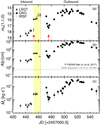 |
Fig. 1 (a) Absolute magnitudes mR(1, 1, 0), (b) Afρ, and (c) dust mass-loss rate Ṁd of 252Pobserved from UT 2016 February 13 to June 10 with LSGT/SBIG ST-10 (filled triangles), OAO-50/MITSuME (filled circles), and IRSF/SIRPOL (open circles) are shown as a function of the Julian date (JD). The dashed vertical lines denote perihelion at rH = 0.996 au on UT 2016 March 15.28. The two arrows in panel a indicate the presumed locations where 252P presented significant brightness enhancements. In panel b the horizontal line of Afρ = 0.6 denotes the median Afρ value of the comet in the 2000 apparition (Ye et al. 2016b). The two crosses are from the Hubble Space Telescope data of Li et al. (2017) observed within the aperture radius of ≲10 km from the center in the F625W filter. The shaded area (in yellow) covers the epoch of our polarimetric observations. |
3.2 Photometric results II: NIR dust color
From the I of the IRSF data (Eq. (1)), we obtained the colorimetric results of 252P dust. Figure 3 shows the temporal evolution of the mIRSF difference of J−H and H−KS as black and purple circles, respectively. Values of the magnitude differences calculated from mIRSF in Table 1 are listed in Table 2. Overall, the temporal evolution in the NIR dust color of 252P appears to be in opposition to that of the comet’s brightness. Before the activation (March 04.84), the J− H dust color was 0.68 ± 0.26 mag, which is consistent with the color range of cometary dust measured by Jewitt & Meech (1986). Soon after the ignition, both J− H and H− KS values first decreased to the minima: from 0.69 ± 0.20 mag (March 09.85) and 0.50 ± 0.16 mag (March 11.76) to −0.07 ± 0.16 mag (March 12.89) and −0.10 ± 0.16 mag (March 13.82) for J−H, and from 0.20 ± 0.19 mag (March 09.85) and 0.16 ± 0.22 mag (March 11.76) to −0.38 ± 0.16 mag (March 12.89) and −0.07 ± 0.15 mag (March 13.82) for H−KS. The bluest color (i.e., minimal mIRSF difference) occurred on March 12–13 both for J−H and for H−KS, when the comet showed the maximum brightness (Fig. 1a). Subsequently, the colors returned to the pre-activation values: 0.45 ± 0.20 mag (March 14.78) and 0.47 ± 0.19 mag (March 15.83) for J−H, and 0.14 ± 0.22 mag (March 14.78) and 0.12 ± 0.21 mag (March 15.83) for H−KS.
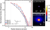 |
Fig. 2 Azimuthally averaged surface brightness profiles of 252P from the (a) LSGT (R band) and IRSF (H band; StokesI) data. All brightness points are normalized to the radial distance of 1.25′′. The black solid and dashed lines denote the gradients of m = −1 and m = −1.5, respectively, which are typical of cometary dust steadily expanding with initial ejection velocity under the solar radiation field (Jewitt & Meech 1987). 2 × 2 binned H-band images are shown, each of which are from (b) before and (c) after the first activation of 252P taken from IRSF. Brightness was normalized between 0 and 1. North is up, and east is to the left. The bottom solid lines scale with 15′′, and the dashed and solid arrows denote the antisolar (−r⊙) and negativevelocity (−v) vectors, respectively. Central stars mark the position of the nucleus. |
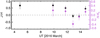 |
Fig. 3 Temporal evolution of the NIR color indices (mdiff) of 252P dust measured from the IRSF data (Table 1). Black and purple circles denote the colors of J− H and H−KS, respectively. |
3.3 Polarimetric results I: phase angle dependence
Low albedos and porous aggregate structures of cometary dust particles have led to a general dependence of P with respect to the scattering plane (Pr) on the phaseangle α, parameterized by a shallow branch of negative polarization with an average minimum polarization Pmin ≈ −1.5% at αmin ≈ 10°, an inversion angle α0 at α ≈ 22°, and a maximum polarization Pmax ≈ 25–30% at αmax ≈ 95° in the optical and NIR (Kiselev et al. 2015).
To investigate the polarimetric behavior of 252P, we first gleaned the archival NIR polarimetric data of cometary dust from the database of comet polarimetry (DOCP; Kiselev et al. 2010, as shown in Fig. 22.3 of Kiselev et al. 2015) and later literature (Kuroda et al. 2015; Kwon et al. 2017). Fitting the average phase curve in each NIR band was obtained by employing the empirical trigonometric function of Penttilä et al. (2005),
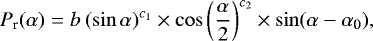 (11)
(11)
where b, c1, c2, and α0 are the wavelength-dependent parameters for characterizing the Pr –α dependence. The best fit (minimum χ2) parameters weighted by the square of the errors in the J, H, and K (KS) bands are described in the captions of Figs. 4–6, respectively. We consider the fitting results of the inversion angle and maximum polarization degrees to be less reliable because of the little data, or lack of data, observed at small (α ≲ 25°) and large (α ≳ 110°) phase angle regions, despite the small fitting errors. Figures 4– 6 present Pr of comets in the J, H, and K (and KS) bands, respectively, as a function of phase angle α. The average α dependences are shown as the solid curves with shaded 3σ areas. The curves are basically the results of interpolation; thus, the error ranges of the four fitting parameters are not as large, except for the case of the J band where there are no available data points at α < 30°. In this case, we forced the curve to fit the point (0, 0) just for visualization.
At first glance, the Pr values of cometary dust are distributed quite homogeneously along the average phase curves, especially in the K and KS bands, regardless of the dynamical class of comets or the observational conditions (e.g., the observing geometry). The similarity in Pr may imply that dust grains of comets have similarities to a large extent in their physical (e.g., structure and size distribution) and/or compositional properties (e.g., complex refractive index). After a careful examination, however, we found that some comets still show deviations from the average trends. In particular, long-period comet C/1995 O1 (Hale–Bopp) consistently shows higher Pr (α) values than the majority of comets in all NIR bands (Jones & Gehrz 2000) or even in the optical (Kwon et al. 2017), whereas short-periodcomets 10P/Tempel 2 and 55P/Tempel-Tuttle (Kelley et al. 2004) apparently have slightly lower Pr (α) values than the average in the K band.
It is noteworthy that 252P showed an abrupt change in Pr (α) during our observations, especially before and soon after the sudden activation on March 04–05. In Figs. 4 and 5, Pr values on March 04 (i.e., before the first activation) were significantly lower (by ~7% in the J and by ~5% in the H bands, but no available KS band data due to the low S/N of < 3) than the expected Pr at given α (i.e., the fitted curves). Throughout the activation, however, Pr increased by ~13% to the maxima on March 12–13. The Pr at perihelion (α ≈ 87° on March 15.38) seems to return to normal. Such a temporal Pr (α) change of the comet looks similar to the patterns of photometrically driven parameters (i.e., mR, Afρ, and Ṁd; see Sect. 3.1).
The polarization vectors of the comet (θr) were roughly aligned perpendicular to the scattering plane (within 4.6° − 10.9° from the normal direction to the scattering plane) in the J, H, and KS bands, but presented a decreasing trend as α increased (θr in Table 1). It should be expected that a randomly distributed scattering medium tends to signal its strongest intensity of the polarized light to the normal direction of the scattering plane (i.e., θr ~ 0°; Bohren & Huffman 1983). Breaking this condition of coma dust might lead to a nonzero value and some systematic trends of θr; however, we could not provide a conclusive explanation for this phenomenon from our results. It might be due to an increase in the accuracy of measurements with increasing values of the Stokes parameters. Alternatively, one of the causes might come from a substructure in the coma of 252P, indecomposable by the aperture polarimetry in this study. A series of high-resolution images taken by Hubble Space Telescope (HST) on March 14 and April 04 2016 suggest that 252P had a strong sunward jet, the influence of which vanished at an aperture size of more than 50–60 pixels (corresponding to 80–100 km in radial distance). As mentioned in Sect. 2.2, our aperture size integrated all signals within the projected radial distances of 82 km (on March 04) to 173 km (on March 15) during the observations, which is similar to or slightly larger than the jet scales.
Near-infrared photometric and polarimetric color indices of 252P/LINEAR from the IRSF data.
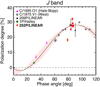 |
Fig. 4 Pr of comets in the J band (λC = 1.25 μm) as a function of phase angle. The data for comets C/1995 O1 (Hale–Bopp), C/1975 V1 (West), and 1P/Halley are from the database of comet polarimetry (DOCP; Kiselev et al. 2010), and the data for comets 209P/LINEAR and C/2013 US10 (Catalina) are from Kuroda et al. (2015) and Kwon et al. (2017), respectively. The red symbols show the results for 252P. The solid curve denotes the interpolated average α dependence of the comets, as a result of Eq. (11). The shaded area (in pink) covers the 3σ region of the average trend. The best fit (minimum χ2) parameters weighted by the square of the errors in J band are b = 38.64 ± 1.74%, c1 = 0.77 ± 0.31, c2 = 0.70 ± 0.11, and α0 = 21.85° ± 2.02°. |
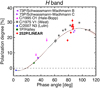 |
Fig. 5 Same as Fig. 4, but in the H band (λC = 1.65 μm). All the comet data except those for 252P are from the DOCP. The best fit (minimum χ2) parameters weighted by the square of the errors in H band are b = 26.57 ± 0.16%, c1 = 0.63 ± 0.04, c2 = (3.41 ± 0.14) × 10-9, and α0 = α0 = 18.76° ± 0.41°. |
 |
Fig. 6 Same as Fig. 4, but in the K and KS bands (λC = 2.20 and 2.25 μm, respectively). All comet data with the exception of those for C/2013 US10 (Catalina) (Kwon et al. 2017) and 252P are quoted from the DOCP. The best fit (minimum χ2) parameters weighted by the square of the errors in K and KS bands are b = 31.47 ± 0.18%, c1 = 0.65 ± 0.06, c2 = (6.55 ± 0.18) × 10-10, and α0 = 16.97° ± 0.44°. |
3.4 Polarimetric result II: spectral dependence
In addition to the α-dependence, Pr exhibits spectral dependence (called polarimetric color, PC), which is defined as
 (12)
(12)
where Pr (λ1) and Pr (λ2) are the Pr values in percent measured at the center wavelengths of λ1 μm and λ2 μm, respectively, and Δλ is the difference between the two wavelengths (λ2 -λ1, when λ2 > λ1) in μm. Positive PC is conventionally labeled in red, and negative PC is labeled blue. PC also depends on the phase angle, but in general the PC of cometary dust is red over λ = 0.5–1.6 μm and seems to turn blue at longer wavelengths at α > 25° (Kolokolova et al. 2004).
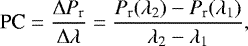
Figure 7 shows the polarimetric color of 252P from the IRSF data. A sequence of the observation epochs and corresponding phase angles are shown on the left and right sides of the data points, respectively. Red on the fourth epoch (March 12) indicates the day when 252P showed the maximum NIR brightness during the IRSF observation (Fig. 1a). The derived values of the PC and their errors are listed in Table 2. Before the activation, the PC was nearly neutral (1; March 04). After the activation (2–7; March 09–15), however, the blue PC became dominant over the J and H bands (i.e., −2.55% μm-1 on average), while the neutral to blue PC was shown over the H and KS bands (i.e., −0.26% μm-1 on average), except for the steep negative slope of the PC at the fourth epoch (4; red line on March 12).
The blue-dominating PC of 252P over the J and H bands is distinctively different from that of other comets observed at high phase angles, which showed a moderate Pr increase at this domain (e.g., ~2.9% μm-1 for comet 1P/Halley at α = 65° and ~3.1% μm-1 for comet C/1975 V1 (West) at α = 66°; Kiselev et al. 2015). Overall, 252P exhibits similar blue PC trends at NIR during the activation, except for the steepest negative PC over the H and KS bands at the fourth epoch (red points) when the comet exhibited the maximum brightness with the highest Pr in shorter wavelengths (open circles in Fig. 1a). Plausible scenarios to produce the observed polarimetric properties of the comet, together with the colorimetric behaviors, will be discussed in Sect. 4.1.
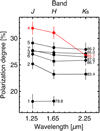 |
Fig. 7 Pr of 252P from the IRSF data (Table 1) as a function of the wavelength. The numbers on the left side of the data indicate the order of the observation epochs (1: March 04, 2: March 09, 3: March 11, 4: March 12, 5: March 13, 6: March 14, and 7: March 15), and the numbers on the right side are the phase angles of the corresponding epochs. Red on the fourth epoch (March 12) denotes the day when the comet shows the maximum NIR brightness (open circles in Fig. 1a). |
4 Discussion
In this section, we search the most likely scenario on the abrupt changes in the NIR dust color and polarimetric properties of 252P we observed and finally discuss its implication on the surface maturity of the comet.
4.1 Abrupt change in polarization degrees near the first activation
As shown in Sects. 3.3 and 3.4, both NIR polarization degree Pr and polarimetric color PC of 252P precipitously changed upon the first activation point only within the change in δrH = 0.008 au, which is one of the biggest and most rapid changes ever observed. It is reminiscent of comet D/1999 S4 (LINEAR), a totally disintegrated comet whose Pr in the optical increased sharply around its perihelion (Kiselev et al. 2002). By definition, Pr is the ratio of the difference of light intensities measured between perpendicular and parallel directions against the scattering plane to the total intensity. A change in Pr thus indicates a change in the physical and/or compositional properties of the dust particles responsible for light scattering as the comet approaches the Sun. Since we observed the comet with the identical instrument in simultaneous multiband imaging polarimetric modes, thereby correcting the systematic effects, it is likely that we detected the real phenomena. We considered three cases that could affect the polarimetric variations, together with the NIR colorimetric results (Sect. 3.2): changes in the (i) composition, (ii) effective size, and (iii) porosity of dust particles.
4.1.1 Change in composition of dust particles
The primary constituents of cometary dust are silicates (mainly in the form of olivine and pyroxene), carbonaceous materials (amorphous carbon and organics), Fe-bearing sulfides, and ice (Levasseur-Regourd et al. 2018). Unlike asteroids, the optical properties of which are largely differentiated with respect to heliocentric distance (DeMeo & Carry 2014; Belskaya et al. 2017), comets seem to possess fairly homogeneous bulk optical properties with a low geometric albedo of ~0.04 (Lamy et al. 2004), showing a nearly uniform distribution on the polarimetric phase curves, regardless of dynamical classes (Kwon et al. 2017). However, any difference in a comet might be expected if we consider the grain properties with depth in the nucleus, perhaps as a result of mainly solar irradiation on the outer layers. Notably, solar heating tends to deplete near-surface volatiles (e.g., Prialnik et al. 2004), which means that the observed discontinuous brightening of 252P (Sect. 3.1) and its jet structure detected in high-resolution images (Li et al. 2017) during the 2016 apparition might provide a possibility for fresh particles to be ejected from the interior of the nucleus.
Laboratory experiments and numerical modeling of comet analogs showed that changes in dust compositioncould make a difference to total absorptivity, which leads to a change in polarimetric properties: particles that are more transparent are subject to multiple scattering, so that the scattered light would be more depolarized. Absorptive particles, however, suppress the multiple scattering, which results in higher Pr. Hence, increasing absorption with wavelength may lead to red PC, whereas decreasing absorption with wavelength may cause blue PC while leaving all other properties (i.e., size and porosity) unchanged (Gustafson & Kolokolova 1999; Kolokolova et al. 2001, 2004; Kimura et al. 2006 and references therein).
Therefore, to satisfy the observed increase in Pr of 252P, first, the ejection of more absorptive particles is required. For carbonaceous materials, their absorption coefficients on wavelength increases in the NIR (Rouleau & Martin 1991; Greenberg & Li 1996; Kolokolova & Jockers 1997), such that they produce a red PC and not our observed blue PC. On the contrary, the ejection of the compact icy or solid absorbing particles (Warren 1984, 2019), whose scattering largely depends on the single scattering of the whole particles but not as much on the absorption coefficients as fluffy ones (Kolokolova & Jockers 1997; Gustafson & Kolokolova 1999), allows them to contribute to the increase in Pr and probably to the blue PC if the size of the particles is larger than a few tens of μm (see Sect. 4.1.2 for detail discussions on the size and porosity). The idea of the ejection of compact icy particles during the discontinuous brightening around perihelion might be reconciled with the existence of sintered subsurface icy layer (Kossacki et al. 1994, 2015). Meanwhile, the bluing of the NIR color data (Sect. 3.2) could provide the additional constraint, if this is a purely compositional effect, that more transparent materials were ejected during the activation. However, the dominance of such material is incompatible with the sharp increase in Pr, which indicates that factors other than the compositional effect should be the primary cause of the NIR color agent.
In summary, variations in the composition of dust particles may not be a primary factor provoking the sudden change in polarimetric parameters of the 252P preperihelion, but instead other properties, such as porosity and size of dust particles, should be considered as the factors responsible for the observed phenomena of the comet.
4.1.2 Change in particle size and porosity
Scattering regimes can be broadly classified into three types depending on the size parameter X of dust (X:= 2πa∕λ, where a is the particle radius and λ is the observation wavelength): the Rayleigh, Mie, and geometrical optics regimes in order of increasing a. Relatively high Pr (α) can be achieved in the regimes of the Rayleigh (X ≪ 1; a ≪ 0.2 μm in the J, a ≪ 0.3 μm in the H, and a ≪ 0.4 μm in the KS bands) and geometrical optics (X ≫ 10; a ≫ 2.0 μm in the J, a ≫ 2.6 μm in the H, and a ≫ 3.6 μm in the KS bands).
For Rayleigh-like tiny particles in the Mie scattering regime (X ~ 1–10; an order of 0.1–1 μm dust in the NIR), the greater their contribution to the scattered light, the higher the observed Pr (α) and the redder PC (Kolokolova et al. 2004). Unfortunately, the dominance of such particles would not explain the observed results for 252P, particularly the observed bluing of the NIR dust color (Fig. 3) and the prevailing blue PC over the J and H bands upon the activation (Fig. 7), and seems to conflict with the results of previous studies showing a minor role of very small particles in mass density (i.e., dynamics) (Fulle et al. 2015, 2016; Rotundi et al. 2015), and in light scattering of cometary dust (Jewitt & Meech 1986; Kolokolova et al. 2007). Therefore, we dismiss the possibility that the observed polarimetric changes were largely stimulated by the increase in Rayleigh (or Rayleigh-like) particles, although not ruling out their possible existence evidenced by the change in the optical brightness (Sect. 3.1) and observed jet-like structure in the optical (Li et al. 2017). Meanwhile, such small dust particles may thermally depolarize the KS -band data (e.g., blue PC over the H and KS bands in Fig. 7), but we preclude the predominance of such a possibility based on the Pr (α) of 252P in the KS band near perihelion having similar values to the points of comet C/1975 V1 (West) (gray squares; Oishi et al. 1978) from which thermal flux was subtracted and based on the case of C/1975 V1 (West), whose thermal depolarization effect was negligible at rH ≳ 0.9 au (Oishi et al. 1978).
Large dust particles in the geometrical optics regime (a > a few tens of μm) can be further considered with two different porosities: fluffy (porous) and compact particles, which are in fact the two main populations of dust particles of comet 67P/Churyumov-Gerasimenko (67P) collected by Rosetta/GIADA (Fulle et al. 2015). In the case of large fluffy particles – with tensile strength of <105 N m-2 (Mendis 1991) and high charge-to-mass ratio (Fulle et al. 2015) – they behave similarly to individual constituent particles in dynamics (Mukai et al. 1992), in light scattering (Kolokolova 2011), and in thermal emissions (Wooden 2002; Kolokolova et al. 2007). Accordingly, the polarimetric properties of scattered light by such large fluffy dust particles would be similar to those by particles approaching the Rayleigh regime (but are larger than X = 1) (i.e., an increase in Pr with the redPC), which again contradicts the observed results of 252P.
Finally, we consider to what extent large compact dust particles contributed to the observed polarimetric properties of 252P. A dominance of these particles was corroborated by the results of Rosetta/GIADA, showing that millimeter- to centimeter-sized compact chunks of 67P ejected near perihelion, along with the release of the upper desiccated layer with a higher refractory-to-ice mass ratio than that inside the nucleus, accounted for >85% of the dust mass-loss and luminosity function of the comet (e.g., Blum et al. 2017; Fulle et al. 2018). As the interaction energy between ambient dipoles (i.e., monomers) are inversely proportional to the cube of the distance between the two (Jackson 1962), less porous materials are more subject to the scattered light from neighboring dust constituents. Accordingly, as the wavelength of the incident light increases (i.e., more monomers are covered in a single wavelength), the Pr of such compact particles decreases more rapidly than that of the porous particles due to the enhanced electromagnetic interaction (Gustafson & Kolokolova 1999; Kolokolova & Kimura 2010). Compared to the nonperiodic and long-period comets observed at similar phase angles, it is more likely that the near-surface of 252P has a paucity of small fluffy dust particles owing to its more frequent perihelion passages in the near-Earth orbit (e.g., Li & Greenberg 1998; Kolokolova et al. 2007). The circumstance would emerge as the unusual blue PC of the comet. For this reason the dominance of signals by the ejection of large compact particles into the coma would be attributable to both a sudden increase in Pr and the enhanced blue PC upon the first activation of 252P.
4.1.3 Tentative conclusions on particle properties ejected during the activation
The ejection of particles that are large (i.e., a is at least greater than a few tens of μm in the geometrical optics regime) and compact (likely as low as the porosity of ~30–65% of the near-surface Rosetta/Philae landing site of 67P; Spohn et al. 2015) can also be deduced from the morphology of the dust coma and the color change of the apparent magnitudes of the IRSF data. Figure 2c shows a broad extension of the dust cloud to the trailing direction (-v) with respect to the photocenter, alluding to the ejection of dust particles that are insensitive to the solar radiation pressure at rH ≲ 1 au. This means that the primary factor that distributes the ejected particles in the -v direction should instead be an explosive mechanism, such as a rocket force from sublimating gas with nonzero ejection velocity (Kelley et al. 2013), which is most likely responsible for the discontinuous brightening of the comet. Concurrently, the J− H and H− KS colors of the comet decreased with time (Fig. 3) from the typical color of cometary dust before the activation (e.g., Jewitt & Meech 1986) to the blue–neutral color. It may also support our scenario that the dust particles that are brighter at the longer wavelengths contributed more to the intensity of the comet than the smaller or large porous dust particles. Taken as a whole, the above conjectures may answer our first question: the evolved near-surface dust layer would primarily define the activity of the comet as long as the incoming solar heat flux is sufficiently large.
4.2 Implication for evolved surface
Our second question is how useful NIR polarimetry would be to discriminate the behaviors of fresh and evolved dust particles. The discussion on the observed polarimetric properties largely induced by the evolved dust particles of 252P in Sect. 4.1 could advocate for the potential usefulness of this approach.
Returning to Fig. 6, the Pr (α) of 11 comets in the K band, where the number of observed comets is to date the highest among the NIR bands, follows the average trend quite well, while a careful check reveals that nonperiodic or long-period comets tend to show, on average, higher Pr (α) values, particularly than two Jupiter-family comets (JFCs), 10P/Tempel 2 and 55P/Tempel-Tuttle (Kelley et al. 2004). Interestingly, the two are characterized by weak to absent 10 μm silicate emission features and a slight temperature excess for the blackbody temperature (Lynch et al. 1995, 2000), both suggesting alack of small (micrometer-sized) and/or fluffy dust particles (Hanner 1999; Wooden 2002; Lisse et al. 2002). Given that JFCs orbit closer to the Sun (which offers a more favorable environment to develop the consolidated dust mantles on their surfaces) than nonperiodic or long-period comets, it would be understandable for JFCs to show lower Pr (α) at NIR thanthose of less-heated comets. The orbital evolution of 252P in the near-Earth orbit over 300 yr or even more would be in favor of this scenario(Appendix B). However, for the moment, we should be cautious before drawing any firm conclusions. A single Pr (α) point of a comet does not provide much information on its physical and compositional properties, but rather, we need (quasi-)simultaneous multiband polarimetric data to measure the PC of dust particles for estimation of the porosity of dust and/or comets observed at multiple observation epochs, including the high-α region, to trace the variation of the Pr (α) and PC. Further NIR polarimetric observations undertaken in a well-organized manner are highly desirable in order to investigate secular evolutions of polarimetric parameters of cometary dust on the orbital motion and to search for any systematic differences in them between different dynamical groups of comets.
5 Summary
We presented multiband NIR imaging polarimetric observations around the perihelion passage and optical imaging observationsof comet 252P/LINEAR taken over four months in its 2016 apparition. We summarize the main results as follows:
- 1.
We detected two discontinuous brightness enhancements of 252P: one in the inbound orbit (on UT 2016 March 04–05) and the other in the outbound orbit (March 27–28). A month prior to the perihelion passage, 252P already showed ~13 times higher Afρ values than those of the 2000 apparition.
- 2.
Upon the first activation, mR(1, 1, 0) and Afρ of 252P derived from the optical R and RC bands data increased by ~2 mag and ~35 cm, respectively. The attendant Ṁd for the assumed 1 μm particles increased to ~5.5 times the initial state. In the meantime, the J−H and H−KS dust color values of 252P had both decreased, showing the bluest color in the middle of the activation.
- 3.
Before the first activation, the Pr values of 252P were far lower than the average trend of comets at given α, by ~7 and ~5% in the J and H bands, respectively. Upon and soon after the activation, however, the Pr increased in all NIR bands by ~13% at most, showing the distinctive development of the blue PC over 1.25–2.25 μm similar to but stronger than the behaviors of a fragmenting comet D/1999 S4 (LINEAR) (Kiselev et al. 2002). In particular, the blue-dominating PC at the J–H bands (−2.55% μm-1 on average) is different from other comets observed, which show moderately red PC values at similar phase angles.
- 4.
The most likely implication of the sudden change in the observed polarimetric properties of the comet during the activation (i.e., increased Pr with theblue PC) and the bluing of the NIR dust color would be the dominance of large (i.e., well located in the geometrical optics regime at NIR) compact particles predominantly ejected from the desiccated dust layer. The paucity of small fluffy dust particles around the nucleus of 252P would be ascribed to the more intense solar heating effects the comet has received in the near-Earth orbit (Appendix B) than for the less-heated nonperiodic or long-period comets observed to date.
Acknowledgements
We thank the referee, L. Kolokolova, whose careful reading and constructive comments improved our manuscript. Y.G.K. was supported by the Global Ph.D. Fellowship Program through a National Research Foundation of Korea (NRF) grant funded by the Ministry of Education (NRF-2015H1A2A1034260). This work at Seoul National University was also supported by the NRF funded by the Korean Government (MEST) grant No. 2018R1D1A1A09084105. J.K. was supported by Astrobiology Center of NINS. MI and CC acknowledge the support from the National Research Foundation of Korea (NRF) grant No. 2017R1A3A3001362. M.T. was supported by MEXT/JSPS KAKENHI grant Nos. 18H05442, 15H02063, and 22000005. The IRSF project is a collaboration between Nagoya University and the South African Astronomical Observatory (SAAO) supported by Grants-in-Aid for Scientific Research on Priority Areas (A; No. 10147207 and No. 10147214) and Optical & Near-Infrared Astronomy Inter-University Cooperation Program, from the Ministry of Education, Culture, Sports, Science and Technology (MEXT) of Japan and the National Research Foundation (NRF) of South Africa.
Appendix A Postperihelion activation of 252P
A.1 Photometric results
Changes in the postperihelion activity level of 252P were quantified by the photometry, as in Sect. 3.1. The intrinsic brightness of 252P (Fig. 1a; derived from Eq. (7)) soon after perihelion passage seemed to decline steeply, but it began to rebound from the minimum of ~17.3 mag with a flux increase of nearly 16 times on UT 2016 March 27–28 (right arrow in Fig. 1a). Such re-ignition again became tranquil after peaking in approximately late April to early May at ~14.3 mag. The changes in Afρ and Ṁd patterns also showed similar trends with that of mR(1, 1, 0), even though the first two have their maxima ~ a week after the peak of mR (1, 1, 0).
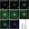 |
Fig. A.1 Wide-field composite images of 252P from the multiband OAO data. In each panel, the observation date and 5′ scale bar are given at the top and bottom left, respectively. Denotations of arrows are identical with those in Fig. 2. North is up, and east is to the left. Green, blue, and red hues represent the fluxes in the g′, RC, and IC bands, respectively. We note that the applied photometric aperture size of 1000 km in radius during this period decreased from 33.6′′ to 2.5′′, which is much smaller than the field of view of each panel. |
Over 1.5 months after the second activation, the Afρ values of 252P (Fig. 1b; derived from Eq. (8)) increased ~57 times from 14.1 ± 3.8 to 808.7 ± 17.6 cm. We compared the Afρ values with the HST data in the broadband F625W filter (λC = 0.625 μm) taken on UT 2016 March 14 and April04 (16.8 ± 0.3 cm and 57 ± 1 cm, respectively, from Li et al. 2017; cross points in Fig. 1b). There are consistent differences of ~20 cm between the HST and OAO data observed at similar epochs, but we suspect that the different photometric aperture sizes employed (more than two orders of magnitude, i.e., ρ ≲ 10 km for the HST data and ρ = 1000 km for the OAO data) might cause the difference in Afρ. Although, by definition, Afρ should be a constant value regardless of the aperture size under the steady expansion in the coma, such a condition would not be met in the vicinity of the nucleus. Considering that Afρ increases outward to reach an equilibrium (to ~1000 km at rH ~ 1 au; see, e.g., Bonev et al. 2008), it might be explainable that the OAO data in this study consistently showed higher Afρ than those of the HST data. Nonetheless, the HST data can be interpreted in line with the OAO data, in that Afρ of 252P in postperihelion was higher than that in preperihelion.
Similarly, variations in Ṁd (Fig. 1c; derived from Eqs. (9) and (10)) strongly support the postperihelion reactivation of 252P, although the overall morphology of the evolutionary trend follows a concave shape, increasing and decreasing both in proportion to the third power of rH, unlike the convex shapes of the mR(1, 1, 0) and Afρ trends. From the minimum of 1.1 ± 1.0 kg s-1 on March 27 through the maximum of 31.3 ± 2.1 kg s-1 on May 02 to another minimum of 4.5 ± 2.4 kg s-1 on June 10, the total mass-loss during the second activation event was ~7.8 × 10⁷ kg, when we assumed nominal ā = 1 μm dust grains. Taken as a whole, the derived parameters indicate that the second activation of 252P was likely on UT 2016 March 27–28.
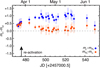 |
Fig. A.2 Temporal evolution in the postperihelion absolute magnitudes of 252P from the multiband OAO data. mX denotes the absolute magnitude in X band, with an aperture size of 1000 km (corresponding to 33.6′′ –2.5′′) in radius. Differences in mX between two bands are shown as blue (mg’ − |


A.2 Variation in the coma color
As a byproduct of our multiband imaging observation, we produced color images to clarify to what extent the fluxes from each band contributed to the postperihelion reactivation of the comet. The g′, RC, and IC band images were allocated as green, blue, and red hues, respectively. Since we employed the broadband filters, gas contamination in flux estimation would be inevitable, particularly by the molecular emissions of the C2 Swan bands in the g′ filter, NH2 α bands in the RC filter, and CN red bands inthe IC filter (Meech & Svoreň 2004).
Figure A.1 presents wide-field composite images, together with the dates of observation and 5′ scale bars in each panel, the fields of view of which are much larger than the applied photometric aperture size. These images show that greenish and bluish components spherically expanded from the nucleus once the comet became activated, whereas a whitish component elongated along the antisolar direction (−r⊙). As the activity of the comet peaked, a greenish coma covered the entire field of view, developing a significant bluish greencolor in the innermost coma. The gas coma of 252P at this term spherically extended to >104 km from the nucleus in the sky plane (panels d to f). Meanwhile, a reddish component was observably dominant, only after the reactivating event was completed (panel h).
Figure A.2 shows the temporal evolution of the 252P coma color in postperihelion more quantitatively. All reduced magnitudes were derived with the 1000 km aperture size (corresponding to 33.6′′–2.5′′) in radius, the central most regions from the nucleus of each panel in Fig. A.1. The magnitude differences between the g′−RC and RC −IC bands are given as blue (mg’ −  ) and orange (
 −
−  ) circles, respectively. The putative activation point (on March 27–28) is marked as an arrow. Overall, a blueward color change (i.e., predominant brightening in the RC band flux) is apparent in the inner coma. Before the activation, the comet was slightly red, showing on average mg’ −
  ~ 0.5 and
  −
−  ~ 0.4 (almost identical within the error bars, however), which are physically indistinguishable from those of short-period comets in the inner solar system (Solontoi et al. 2012). During the activation, however, fluxes in the RC band became significantly enhanced, resulting in the redder color of mg’ −
  and more neutral color of
  −
−  . These magnitude differences remained nearly constant at the value of mg’ −
  = 0.9 ± 0.1 (the standard deviation of the nominal values) and
  −
−  = 0.2 ± 0.1 over the following 1.5 months. After peaking, the maximum Afρ and Ṁd, the coma color again turned to reddish-neutral, albeit with large uncertainties, consistent with the status before the activation.
Appendix B Orbital evolution of 252P/LINEAR and its dynamical association with P/2016 BA14 (PanSTARRS)
In this section, we present our investigation of orbital evolution of 252P and its dynamical association with P/2016 BA14 (PanSTARRS) to search for any possible dynamical characteristics of the objects attributable to the observed photo-polarimetric properties of 252P.
Comet P/2016 BA14 (PanSTARRS; hereafter BA14), a possible dynamical pair of 252P with remarkably similar orbital elements (Rudawska et al. 2016), possesses a geometric albedo of <3% (Reddy 2016) and diametric size of >1 km (Naidu et al. 2016) or 1–2 km (Li et al. 2017). Unlike the capricious behavior of 252P, BA14 showed an r′ -band magnitude that was more than 6 mag larger with a fraction of active area on the surface of ~0.01%, (i.e., it was rather asteroidal in the 2016 apparition) (Li et al. 2017). To trace the dynamic history of the two back to the time when they were ejected into the near-Earth orbit, we conducted a backward dynamical simulation with the Mercury 6 integrator (Chambers 1999) under the gravity of the Sun and eight planets. We generated 1000 clones randomly distributed within the 1σ Gaussian distribution, with the orbital elements quoted on the JPL Small-Body Database Browser site. They were integrated 1000 yr backwardwith an 8-day time step in the general Bulirsch–Stoer mode without considering the Yarkovsky force (i.e., consistent with the negligible activity levels before the 2016 apparition). The applied orbital elements and their errors are summarized in Table 2.
In addition, to assess the orbital similarity of two bodies in the near-Earth orbit, we estimated a traditional DSH parameter (Southworth & Hawkins 1963), which is a distance between the orbits of two bodies in five-dimensional orbital element space (q, e, i, ω, and Ω) calculated as
![\begin{equation*} \begin{aligned} D_{\textrm{SH}} = {} & \Bigg[\big(e_{\textrm{B}} - e_{\textrm{A}}\big)^{\textrm{2}} + \big(q_{\textrm{B}} - q_{\textrm{A}}\big)^{\textrm{2}} \\ & + \bigg(2 \sin \frac{I_{\textrm{AB}}}{2} \bigg)^{\textrm{2}} + \bigg[\big(e_{\textrm{A}} + e_{\textrm{B}}\big) \sin \frac{\Pi_{\textrm{AB}}}{2}\bigg]^{\textrm{2}}\Bigg]^{\textrm{1/2}},\end{aligned} \end{equation*}](/articles/aa/full_html/2019/09/aa35542-19/aa35542-19-eq26.png) (B.1)
(B.1)
![\begin{equation*} I_{\textrm{AB}} = \arccos \Big[ \cos i_{\textrm{A}} \cos i_{\textrm{B}} + \sin i_{\textrm{A}} \sin i_{\textrm{B}} \cos \big(\Omega_{\textrm{A}} - \Omega_{\textrm{B}} \big) \Big]\end{equation*}](/articles/aa/full_html/2019/09/aa35542-19/aa35542-19-eq27.png)
Orbital elements of 252P and BA14 and their 1σ uncertainties at Epoch 2 457 519.5 (=2016 May 11.0).
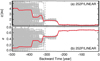 |
Fig. B.1 Time evolution of (a) the perihelion distance q and (b) the eccentricity e of 252P. Red lines denote the evolution of a particle with the average values at the epoch (May 11, 2016, the Julian date of 2 457 519.5), while each gray line represents that of an individual clone, the orbital elements of which follow 1σ standard deviation of the Gaussian distribution. |
![\begin{equation*} \Pi_{\textrm{AB}} = \big(\omega_{\textrm{A}} - \omega_{\textrm{B}} \big) + 2 \arcsin \!\Bigg[\!\!\cos \frac{(i_{\textrm{A}} + i_{\textrm{B}})}{2} \!\sin \!\frac{(\Omega_{\textrm{A}} - \Omega_{\textrm{B}})}{2} \sec \frac{I_{\textrm{AB}}}{2} \!\Bigg].\end{equation*}](/articles/aa/full_html/2019/09/aa35542-19/aa35542-19-eq28.png)
The subscripts A and B denote the two bodies to be compared (A for 252P and B for BA14), q is the perihelion distance in au, e is the eccentricity, i is the inclination, ω is the argument of perihelion, and Ω is the longitude of the ascending node. In the case of DSH ≤ 0.20, we tend to consider that the two bodies are probably within the association range (Southworth & Hawkins 1963). For instance, a minimum DSH value of the possible pair, (3200) Phaethon and 2005 UD, shows ~0.04 (Ohtsuka et al. 2006).
Figure B.1 shows the time evolution of the orbital elements of 252P. Red lines denote the evolution of a particle with the average values at the epoch (May 11, 2016, the Julian date of 2 457 519.5), while each gray line represents that of an individual clone, the orbital elements of which have 1σ standard deviation onthe Gaussian distribution. Our simulation shows that 252P would have closely encountered Jupiter at the minimum distance of dmin ~ 0.02 au, 314 yr ago. Due to the high uncertainty, we could only trace back the orbital evolution of the comet from the current epoch to ~310 yr in the past, during which the q and e of the comet changed by δq ~ −1 au (decreasing) and by δe ~ +0.2 (increasing). Interestingly, based on the current orbital elements of 252P, the Near-Earth Object (NEO) model of Greenstreet et al. (2012) suggests the two most probable source regions of the comet: the JFC source (~81.8%) and the outer main asteroidal belt (~16.2%). In either case, 252P should have eventually been transported to the current orbit by means of the resonance with Jupiter and the perturbations of terrestrial planets (e.g., Morbidelli et al. 2002). Based on the analysis, we conjecture that the decreasing q, together with its repetitive close encounters with planets (e.g., with Jupiter within ~0.05 au at ~320 yr ago and with the Earth within ~0.02 au since ~170 yr to the present), might introduce internal stresses to 252P, which would render the nucleus overall more fragile and would in turn affect the rapid polarimetric variation in its perihelion passage.
The average DSH value derived from the osculating orbital elements of 252P and BA14 is ~0.16, which implies a positive dynamical correlation of two bodies, although not as tight as that of (3200) Phaethon and 2005 UD (Ohtsuka et al. 2006). Among all the possible combinations of the 1σ clones, we obtained the minimum DSH value of ~0.15. Owing to the close encounters of the objects to the planets and their nongravitational force, it is hard to determine from this study exactly when they were fragmented each other.
Appendix C Contrast in behaviors of large and small comet nuclei in the near-Earth orbit
This section describes our conjecture of the reason why 252P and BA14 exhibited such different activity patterns during the 2016 apparition, despite their possible dynamical association resulting in similar orbital evolution in the near-Earth orbit.
The remarkably high activity of 252P in 2016 compared to the previous apparitions, alongside its discontinuous brightness enhancements near perihelion, is far different from the behavior of the comet over the past apparitions. We speculate that the effects of such orbital evolution on comets in near-Earth orbits might vary greatly depending on comet nuclei size. This speculation would be demonstrated by different observational characteristics of 252P and BA14 in the 2016 apparition, despite their similar orbital evolution over a few centuries (i.e., DSH ≤ 0.20 in Appendix B). Comet 252P is on the small end of sizes (300 ± 30 m; Li et al. 2017) of JFCs, for which a typical comet nucleus would range from one to a few kilometers in size (Fernández et al. 1999; Barnes et al. 2019). The surface gravity of 252P would then be less than a factor of at least one-fifth the gravity at the surface of ordinary JFCs. The concomitant smaller escape velocity permits large particles, millimeter to centimeter in size, to readily escape the gravitational influence of 252P, while a larger nucleus would more easily accumulate dust particles on its surface.
The small size can also contribute to the spin evolution of the nuclei such that the rotational stability tends to be proportional to the fourth power of the radius of the nucleus (τex ∝  ; Jewitt 2004). Comet 252P thus has a ≳103 times smaller excitation timescale than that of a typical JFC. Indeed, a sudden increase of nongravitational force of 252P by a factor of ~10, but negligible change of BA14 during the 2016 apparition (Li et al. 2017) may reflect this higher rotational instability of the smaller comet.
Taken as a whole, the consequences of the small nucleus size together with the orbital evolution in the near-Earth orbit (Appendix B) would enhance erratic sublimation patterns of the comet, probably resulting from highly changeable mass transfer on the surface (e.g., landslides; Keller et al. 2017) due to the enhanced solar radiation and/or in unstable development of the dust mantle on the surface (e.g., Rickman et al. 1990). They may in turn affect the abnormal variations of the photo-polarimetric parameters of 252P near its perihelion.
Appendix D Additional tables
Observational geometry and instrument settings.
Photometry of 252P/LINEAR.
References
- A’Hearn, M. F., Schleicher, D. G., Millis, R. L., Feldman, P. D., & Thompson, D. T. 1984, AJ, 89, 579 [NASA ADS] [CrossRef] [Google Scholar]
- Barnes, T. F., A’Hearn, M. F., & Kolokolova, L., (Eds.), Properties of Comet Nuclei (PDS4 Format), urn:nasa:pds:compil-comet:nuc_properties::1.0, NASA Planetary Data System, 2019 [Google Scholar]
- Belskaya, I. N., Fornaxier, S., Tozzi, G. P., et al. 2017, Icarus, 284, 30 [NASA ADS] [CrossRef] [Google Scholar]
- Biele, J., Ulamec, S., Maibaum, M., et al. 2015, Science, 349, aaa9816 [NASA ADS] [CrossRef] [Google Scholar]
- Binney, J., & Merrifield, M. 1998, Galactic Astronomy (Princeton, NJ: Princeton University Press) [Google Scholar]
- Blum, J., Gundlach, B., Krause, M., et al. 2017, MNRAS, 469, 755 [Google Scholar]
- Bohren, C., & Huffman, D. 1983, Absorption and Scattering of Light by Small Particles (New York: Wiley Sons) [Google Scholar]
- Bonev, T., Boehnhardt, H., & Borisov, G. 2008, A&A, 480, 277 [NASA ADS] [CrossRef] [EDP Sciences] [Google Scholar]
- Chambers, J. E. 1999, in Impact of Modern Dynamics in Astronomy, eds. J., Henrard, & S., Ferraz-Mello (Berlin: Springer), 449 [CrossRef] [Google Scholar]
- Chernova, G. P., Kiselev, N. N., & Jockers, K. 1993, Icarus, 103, 144 [NASA ADS] [CrossRef] [Google Scholar]
- Coulson I., M., Cordiner, M. A., Kuan, Y.-J., et al. 2017, AJ, 153, 169 [NASA ADS] [CrossRef] [Google Scholar]
- Curti, R. M., Skrutskie, M. F., van Dyk, S., et al. 2003, VizieR On-line Data Catalog: II/246 [Google Scholar]
- DeMeo, F. E., & Carry, B. 2014, Nature, 505, 629 [NASA ADS] [CrossRef] [Google Scholar]
- Drilling, J. S., & Landolt, A. U. 2000, in Astrophysical Quantities 4th edn., ed. A. N. Cox (New York: Springer), 381 [Google Scholar]
- Fernández, J. A., Tancredi, G., Rickman, H., & Licandro, J. 1999, A&A, 352, 327 [NASA ADS] [Google Scholar]
- Fernie, J. D. 1983. PASP, 95, 782 [NASA ADS] [CrossRef] [Google Scholar]
- Fulle, M., Corte, D., Rotundi, V., et al. 2015, ApJL, 802, 12 [Google Scholar]
- Fulle, M., Altobelli, N., Buratti, B., et al. 2016, MNRAS, 462, 2 [Google Scholar]
- Fulle, M., Blum, J., Green, S. F., et al. 2018, MNRAS, 482, 3326 [Google Scholar]
- Greenberg, J. M., & Li, A. 1996, A&A, 309, 258 [NASA ADS] [Google Scholar]
- Greenstreet, S., Ngo, H., & Gladman, B. 2012, Icarus, 217, 355 [NASA ADS] [CrossRef] [Google Scholar]
- Gundlach, B., Ratte, J., Blum, J., Oesert, J., & Gorb, S. N. 2018, MNRAS, 479, 5272 [NASA ADS] [CrossRef] [Google Scholar]
- Gustafson, B. Å. S., & Kolokolova, L. 1999, J. Geophys. Res., 104, 31711 [NASA ADS] [CrossRef] [Google Scholar]
- Hanner, M. S. 1999, Space Sci. Rev., 90, 99 [NASA ADS] [CrossRef] [Google Scholar]
- Henden, A. A., Templeton, M., Terrell, D., et al. 2016, VizieR Online Data Catalog: II/336 [Google Scholar]
- Im, M., Choi, C., & Kim, K. 2015, J. Korean Astron. Soc., 48, 207 [NASA ADS] [CrossRef] [Google Scholar]
- Ishiguro, M., Watanabe, J.-I., Sarugaku, Y., et al. 2010, ApJ, 714, 1324 [NASA ADS] [CrossRef] [Google Scholar]
- Ishiguro, M., Kuroda, D., Hanayama, H., et al. 2016, AJ, 152, 169 [NASA ADS] [CrossRef] [Google Scholar]
- Jackson, J. D. 1962, Classical Electrodynamics (Hoboken, NJ: John Willey & Sons), 641 [Google Scholar]
- Jester, S., Schneider, D. P., Richards, G. T., et al. 2005, AJ, 130, 873 [NASA ADS] [CrossRef] [Google Scholar]
- Jewitt, D. 2002, AJ, 123, 1039 [NASA ADS] [CrossRef] [Google Scholar]
- Jewitt, D. 2004, Comets II (Tucson: University of Arizona Press), 659 [Google Scholar]
- Jewitt, D., & Meech, K. 1986, ApJ, 310, 937 [NASA ADS] [CrossRef] [Google Scholar]
- Jewitt, D., & Meech, K. 1987, ApJ, 317, 992 [NASA ADS] [CrossRef] [Google Scholar]
- Jones, T. J., & Gehrz, R. D. 2000, Icarus, 143, 338 [NASA ADS] [CrossRef] [Google Scholar]
- Jordi, K., Grebel, E. K., & Ammon, K. 2005, A&A, 460, 339 [Google Scholar]
- Kandori, R., Kusakabe, N., Tamura, M., et al. 2006, Proc. SPIE, 6269, 626951 [CrossRef] [Google Scholar]
- Kato, D., Nagashima, C., Nagayama, T., et al. 2007, PASJ, 59, 615 [NASA ADS] [Google Scholar]
- Keller, H. U., Mottola, S., Hviid, S. F., et al. 2017, MNRAS, 469, 357 [Google Scholar]
- Kelley, M. S., Woodward, C. E., Jones, T. J., Reach, W. T., & Johnson, J. 2004, AJ, 127, 2398 [NASA ADS] [CrossRef] [Google Scholar]
- Kelley, M. S., Lindler, D. J., Bodewits, D., et al. 2013, Icarus, 222, 634 [NASA ADS] [CrossRef] [Google Scholar]
- Kimura, H., Kolokolova, L., & Mann, I. 2006, A&A, 449, 1243 [NASA ADS] [CrossRef] [EDP Sciences] [Google Scholar]
- Kiselev, N., Jockers, K., & Rosenbush, V. 2002, Earth Moon Planet, 90, 167 [NASA ADS] [CrossRef] [Google Scholar]
- Kiselev, N., Velichko, S., Jockers, K., Rosenbush, V., & Kikuchi, S. 2010, NASA Planetary Data System, Database of Comet Polarimetry (DOCP), EAR-C-COMPIL-5-COMET-POLARIMETRY-V1.0, 8124 [Google Scholar]
- Kiselev, N., Rosenbush, V., Kolokolova, L., & Levasseur-Regourd, A.-Ch. 2015, in Polarimetry of Stars and Planetary Systems, eds. L. Kolokolova, J. Hough, & A. Levasseur-Regourd (Cambridge: Cambridge University Press), 379 [Google Scholar]
- Kolokolova, L. 2011, ASPC, 449, 345 [NASA ADS] [Google Scholar]
- Kolokolova, L., & Jockers, K. 1997, Planet. Space Sci., 45, 1543 [NASA ADS] [CrossRef] [Google Scholar]
- Kolokolova, L., & Kimura, H. 2010, A&A, 513, A40 [NASA ADS] [CrossRef] [EDP Sciences] [Google Scholar]
- Kolokolova, L., Jockers, K., Gustafson, B. Å. S., & Lichtenberg, G. 2001, J. Geophys. Res., 106, 10113 [NASA ADS] [CrossRef] [Google Scholar]
- Kolokolova, L., Hanner, M. S., Levasseur-Regourd, A.-C., & Gustafson, B. Å. S. 2004, in Comets II, eds. M. Festou, H. U. Keller, & H. A. Weaver (Tucson: University of Arizona Press), 577 [Google Scholar]
- Kolokolova, L., Kimura, H., Kiselev, N., & Rosenbush, V. 2007, A&A, 463, 1189 [NASA ADS] [CrossRef] [EDP Sciences] [Google Scholar]
- Kossacki, K. J., Kömle, N. I., Kargl, G., & Steiner, G. 1994, Planet. Space Sci., 42, 393 [Google Scholar]
- Kossacki, K. J., Spohn, T., Hagermann, A., Kaufmann, E., & Kührt, E. 2015, Icarus, 260, 464 [NASA ADS] [CrossRef] [Google Scholar]
- Kotani, T., Kawai, N., Yanagisawa, K., et al. 2005, Nuovo Cimento C, 28, 755 [NASA ADS] [Google Scholar]
- Kuroda, D., Ishiguro, M., Watanabe, M., et al. 2015, ApJ, 814, 156 [NASA ADS] [CrossRef] [Google Scholar]
- Kusune, T., Sugitani, K., Miao, J., et al. 2015, ApJ, 798, 60 [NASA ADS] [CrossRef] [Google Scholar]
- Kwon, J., Tamura, M., Hough, J., et al. 2015, ApJ, 824, 85 [Google Scholar]
- Kwon, Y. G., Ishiguro, M., Hanayama, H., et al. 2016, ApJ, 818, 67 [NASA ADS] [CrossRef] [Google Scholar]
- Kwon, Y. G., Ishiguro, M., Kuroda, D., et al. 2017, AJ, 154, 173 [NASA ADS] [CrossRef] [Google Scholar]
- Lamy, P. L., Toth, I., Fernandez, Y. R., & Weaver, H. A. 2004, in Comets II, eds. M. C. Festou, et al. (Tuczon: University of Arizona Press), 223 [Google Scholar]
- Levasseur-Regourd, A. C., Jessica, A., Hervé, C., et al. 2018, Space Sci. Rev., 214, 64 [NASA ADS] [CrossRef] [Google Scholar]
- Li, A., & Greenberg, J. M. 1998, A&A, 338, 364 [NASA ADS] [Google Scholar]
- Li, J. Y., Kelley, M. S., Samarasinha, N. H., et al. 2017, AJ, 154, 136 [NASA ADS] [CrossRef] [Google Scholar]
- Lisse, C. M., A’Hearn, M. F., Fernández, Y. R., & Peschke, S. B. 2002, in Dust in the Solar System and Other Planetary Systems, A Search for Trends in Cometary Dust Emission, IAU Coll. 181, eds. S. F. Green, I. P. Williams, J. A. M. McDonnell, & N. McBride (Canterbury: ASP), 259 [Google Scholar]
- Luu, J. X., & Jewitt, D. C. 1992, AJ, 104, 2243 [NASA ADS] [CrossRef] [Google Scholar]
- Lynch, D. K., Hackwell, J. A., Edelsohn, D., et al. 1995, Icarus, 114, 197 [NASA ADS] [CrossRef] [Google Scholar]
- Lynch, D. K., Russell, R. W., & Sitko, M. L. 2000, Icarus, 144, 187 [NASA ADS] [CrossRef] [Google Scholar]
- McKay, A. J., Kelley, M. S. P., Bodewits, D., et al. 2017, Asteroids, Comets, Meteors, 3b4, http://acm2017.uy/abstracts/Parallel3.b.4.pdf [Google Scholar]
- Meech, K. J., & Svoreň J. 2004, in Comets II, ed. M. Festou, H. U. Keller, & H. A. Weaver (Tucson: University of Arizona Press), 317 [Google Scholar]
- Mendis, D. A. 1991, Astrophys. Space Sci., 176, 163 [NASA ADS] [CrossRef] [Google Scholar]
- Mink, D. J. 1997, in Astronomical data Analysis Software and Systems VI, eds. G. Hunt, & H. E. Payne, ASP Conf. Ser. 125, 249 [NASA ADS] [Google Scholar]
- Morbidelli, A., Bottke, Jr. W. F., Froeschlé, C., & Michel, P. 2002, in Asteroids III, eds. W. F. Bottke, Jr. et al. (Tucson: University of Arizona Press), 409 [Google Scholar]
- Mukai, T., Ishimoto, H., Kozasa, T., Blum, J., & Greenberg, J. M. 1992, A&A, 262, 315 [NASA ADS] [Google Scholar]
- Nagayama, T., Nagashima, C., Nakajima, Y., et al. 2003, Proc. SPIE, 4841, 459 [NASA ADS] [CrossRef] [Google Scholar]
- Naidu, S. P., Benner, L. A. M., Brozovic, M., et al. 2016, in AAS/DPS Meeting 48 Abstract, 219.05 [Google Scholar]
- Ohtsuka, K., Sekiguchi, T., Kinoshita, D., et al. 2006, A&A, 450, L25 [NASA ADS] [CrossRef] [EDP Sciences] [Google Scholar]
- Oishi, M., Kawara, K., Kobayashi, Y., et al. 1978, PASJ, 30, 149 [NASA ADS] [Google Scholar]
- Penttilä, A., Lumme, K., Hadamcik, E., & Levasseur-Regourd, A.-C. 2005, A&A, 432, 1081 [NASA ADS] [CrossRef] [EDP Sciences] [Google Scholar]
- Perovich, D. K. 1998, J. Geophys. Res., 103, 5563 [NASA ADS] [CrossRef] [Google Scholar]
- Prialnik, D., Benkhoff, J., & Podolak, M. 2004, Comets II (Tucson: University of Arizona Press), 359 [Google Scholar]
- Rickman, H., Fernandez, J. A., & Gustafson, B. A. S. 1990, A&A, 237, 524 [NASA ADS] [Google Scholar]
- Reddy, V. 2016, NASA/JPL News, Comet Flying by Earth Observed with Radar and Infrared, 2016 March 24 [Google Scholar]
- Rotundi, A., Sierks, H., Della, C., et al. 2015, Science, 347, aaa3905 [NASA ADS] [CrossRef] [Google Scholar]
- Rouleau, F., & Martin, P. G. 1991, ApJ, 377, 526 [NASA ADS] [CrossRef] [Google Scholar]
- Rudawska, R., Vaubaillon, J., Tóth, J., & Raetz, S. 2016, in AAS/DPS Meeting 48 Abstract, 218.01 [Google Scholar]
- Skrutskie, M. F., Cutri, R. M., Stiening, R., et al. 2006, AJ, 131, 1163 [NASA ADS] [CrossRef] [Google Scholar]
- Solontoi, M., Ivezić, Ž., Jurić, M., et al. 2012, Icarus, 218, 571 [NASA ADS] [CrossRef] [Google Scholar]
- Southworth, R. B., & Hawkins, G. S. 1963, Smithsonian Contributions to Astrophysics (Washington D.C.: Smithsonian Institution), 7, 261 [NASA ADS] [Google Scholar]
- Spohn, T., Knollenber, J., Ball, A. J., et al. 2015, Science, 349, aab0464 [NASA ADS] [CrossRef] [Google Scholar]
- Tancredi, G. 2014, Icarus, 234, 66 [NASA ADS] [CrossRef] [Google Scholar]
- Tokunaga, A. T., Simons, D. A., & Vacca, W. D. 2002, PASP, 114, 180 [NASA ADS] [CrossRef] [Google Scholar]
- Tonry, J. L., Denneau, L., Flewelling, H., et al. 2018, ApJ, 867, 105 [NASA ADS] [CrossRef] [EDP Sciences] [Google Scholar]
- Thomas, H., Ratke, L., & Kochan, H. 1994, Adv. Space Res. 12, 207 [NASA ADS] [CrossRef] [Google Scholar]
- Warren, S. G. 1984, Appl. Opt. 23, 1206 [NASA ADS] [CrossRef] [PubMed] [Google Scholar]
- Warren, S. G. 2019, Phil. Trans. R. Soc. A, 377, 20180161 [NASA ADS] [CrossRef] [Google Scholar]
- Wooden, D. 2002, Earth Moon Planet, 89, 247 [NASA ADS] [CrossRef] [Google Scholar]
- Ye, Q.-Z., Hui, M.-T., Brown, P. G., et al. 2016a, Icarus, 264, 48 [NASA ADS] [CrossRef] [Google Scholar]
- Ye, Q.-Z., Brown, P. G., & Wiegert, P. A. 2016b, ApJ, 818, L29 [NASA ADS] [CrossRef] [Google Scholar]
- Zacharias, N., Finch, C., Girard, T., et al. 2010, AJ, 139, 2184 [NASA ADS] [CrossRef] [Google Scholar]
All Tables
Nightly averaged photometric and polarimetric parameters of 252P/LINEAR taken by IRSF/SIRPOL.
Near-infrared photometric and polarimetric color indices of 252P/LINEAR from the IRSF data.
Orbital elements of 252P and BA14 and their 1σ uncertainties at Epoch 2 457 519.5 (=2016 May 11.0).
All Figures
|
Fig. 1 (a) Absolute magnitudes mR(1, 1, 0), (b) Afρ, and (c) dust mass-loss rate Ṁd of 252Pobserved from UT 2016 February 13 to June 10 with LSGT/SBIG ST-10 (filled triangles), OAO-50/MITSuME (filled circles), and IRSF/SIRPOL (open circles) are shown as a function of the Julian date (JD). The dashed vertical lines denote perihelion at rH = 0.996 au on UT 2016 March 15.28. The two arrows in panel a indicate the presumed locations where 252P presented significant brightness enhancements. In panel b the horizontal line of Afρ = 0.6 denotes the median Afρ value of the comet in the 2000 apparition (Ye et al. 2016b). The two crosses are from the Hubble Space Telescope data of Li et al. (2017) observed within the aperture radius of ≲10 km from the center in the F625W filter. The shaded area (in yellow) covers the epoch of our polarimetric observations. |
| In the text | |
|
Fig. 2 Azimuthally averaged surface brightness profiles of 252P from the (a) LSGT (R band) and IRSF (H band; StokesI) data. All brightness points are normalized to the radial distance of 1.25′′. The black solid and dashed lines denote the gradients of m = −1 and m = −1.5, respectively, which are typical of cometary dust steadily expanding with initial ejection velocity under the solar radiation field (Jewitt & Meech 1987). 2 × 2 binned H-band images are shown, each of which are from (b) before and (c) after the first activation of 252P taken from IRSF. Brightness was normalized between 0 and 1. North is up, and east is to the left. The bottom solid lines scale with 15′′, and the dashed and solid arrows denote the antisolar (−r⊙) and negativevelocity (−v) vectors, respectively. Central stars mark the position of the nucleus. |
| In the text | |
|
Fig. 3 Temporal evolution of the NIR color indices (mdiff) of 252P dust measured from the IRSF data (Table 1). Black and purple circles denote the colors of J− H and H−KS, respectively. |
| In the text | |
|
Fig. 4 Pr of comets in the J band (λC = 1.25 μm) as a function of phase angle. The data for comets C/1995 O1 (Hale–Bopp), C/1975 V1 (West), and 1P/Halley are from the database of comet polarimetry (DOCP; Kiselev et al. 2010), and the data for comets 209P/LINEAR and C/2013 US10 (Catalina) are from Kuroda et al. (2015) and Kwon et al. (2017), respectively. The red symbols show the results for 252P. The solid curve denotes the interpolated average α dependence of the comets, as a result of Eq. (11). The shaded area (in pink) covers the 3σ region of the average trend. The best fit (minimum χ2) parameters weighted by the square of the errors in J band are b = 38.64 ± 1.74%, c1 = 0.77 ± 0.31, c2 = 0.70 ± 0.11, and α0 = 21.85° ± 2.02°. |
| In the text | |
|
Fig. 5 Same as Fig. 4, but in the H band (λC = 1.65 μm). All the comet data except those for 252P are from the DOCP. The best fit (minimum χ2) parameters weighted by the square of the errors in H band are b = 26.57 ± 0.16%, c1 = 0.63 ± 0.04, c2 = (3.41 ± 0.14) × 10-9, and α0 = α0 = 18.76° ± 0.41°. |
| In the text | |
|
Fig. 6 Same as Fig. 4, but in the K and KS bands (λC = 2.20 and 2.25 μm, respectively). All comet data with the exception of those for C/2013 US10 (Catalina) (Kwon et al. 2017) and 252P are quoted from the DOCP. The best fit (minimum χ2) parameters weighted by the square of the errors in K and KS bands are b = 31.47 ± 0.18%, c1 = 0.65 ± 0.06, c2 = (6.55 ± 0.18) × 10-10, and α0 = 16.97° ± 0.44°. |
| In the text | |
|
Fig. 7 Pr of 252P from the IRSF data (Table 1) as a function of the wavelength. The numbers on the left side of the data indicate the order of the observation epochs (1: March 04, 2: March 09, 3: March 11, 4: March 12, 5: March 13, 6: March 14, and 7: March 15), and the numbers on the right side are the phase angles of the corresponding epochs. Red on the fourth epoch (March 12) denotes the day when the comet shows the maximum NIR brightness (open circles in Fig. 1a). |
| In the text | |
|
Fig. A.1 Wide-field composite images of 252P from the multiband OAO data. In each panel, the observation date and 5′ scale bar are given at the top and bottom left, respectively. Denotations of arrows are identical with those in Fig. 2. North is up, and east is to the left. Green, blue, and red hues represent the fluxes in the g′, RC, and IC bands, respectively. We note that the applied photometric aperture size of 1000 km in radius during this period decreased from 33.6′′ to 2.5′′, which is much smaller than the field of view of each panel. |
| In the text | |
|
Fig. A.2 Temporal evolution in the postperihelion absolute magnitudes of 252P from the multiband OAO data. mX denotes the absolute magnitude in X band, with an aperture size of 1000 km (corresponding to 33.6′′ –2.5′′) in radius. Differences in mX between two bands are shown as blue (mg’ − |
| In the text | |
|
Fig. B.1 Time evolution of (a) the perihelion distance q and (b) the eccentricity e of 252P. Red lines denote the evolution of a particle with the average values at the epoch (May 11, 2016, the Julian date of 2 457 519.5), while each gray line represents that of an individual clone, the orbital elements of which follow 1σ standard deviation of the Gaussian distribution. |
| In the text | |
Current usage metrics show cumulative count of Article Views (full-text article views including HTML views, PDF and ePub downloads, according to the available data) and Abstracts Views on Vision4Press platform.
Data correspond to usage on the plateform after 2015. The current usage metrics is available 48-96 hours after online publication and is updated daily on week days.
Initial download of the metrics may take a while.