| Issue |
A&A
Volume 629, September 2019
|
|
|---|---|---|
| Article Number | A14 | |
| Number of page(s) | 10 | |
| Section | Extragalactic astronomy | |
| DOI | https://doi.org/10.1051/0004-6361/201935186 | |
| Published online | 26 August 2019 | |
The XMM-Newton wide field survey in the COSMOS field: Clustering dependence of X-ray selected AGN on host galaxy properties
1
Department of Physics, University of Helsinki, Gustaf Hällströmin katu 2a, 00014 Helsinki, Finland
e-mail: akke.viitanen@helsinki.fi
2
Scuola Normale Superiore, Piazza dei Cavalieri 7, 56126 Pisa, Italy
3
INAF – Osservatorio Astronomico di Roma, Via Frascati 33, 00078 Monte Porzio Catone, Roma, Italy
4
Physics Department, University of Miami, Knight Physics Building, Coral Gables, FL 33124, USA
5
INAF – Osservatorio di Astrofisica e Scienza dello Spazio di Bologna, Via Gobetti 93/3, 40129 Bologna, Italy
6
Instituto de Astronomía, Universidad Nacional Autónoma de México, 22860 Ensenada, Mexico
7
Max-Planck-Institut für extraterrestrische Physik, Giessenbachstrasse 1, 85748 Garching, Germany
Received:
31
January
2019
Accepted:
18
June
2019
Aims. We study the spatial clustering of 632 (1130) XMM-COSMOS active galactic nuclei (AGNs) with known spectroscopic or photometric redshifts in the range z = [0.1–2.5] in order to measure the AGN bias and estimate the typical mass of the hosting dark matter (DM) halo as a function of AGN host galaxy properties.
Methods. We created AGN subsamples in terms of stellar mass, M*, and specific black hole accretion rate, LX/M*, to study how AGN environment depends on these quantities. Further, we derived the M*−Mhalo relation for our sample of XMM-COSMOS AGNs and compared it to results in literature for normal non-active galaxies. We measured the projected two-point correlation function wp(rp) using both the classic and the generalized clustering estimator, based on photometric redshifts, as probability distribution functions in addition to any available spectroscopic redshifts. We measured the large-scale (rp ≳ 1 h−1 Mpc) linear bias b by comparing the clustering signal to that expected of the underlying DM distribution. The bias was then related to the typical mass of the hosting halo Mhalo of our AGN subsamples. Since M* and LX/M* are correlated, we matched the distribution in terms of one quantity and we split the distribution in the other.
Results. For the full spectroscopic AGN sample, we measured a typical DM halo mass of log (Mhalo/h−1 M⊙) = 12.79−0.43+0.26, similar to galaxy group environments and in line with previous studies for moderate-luminosity X-ray selected AGN. We find no significant dependence on specific accretion rate LX/M*, with log (Mhalo/h−1 M⊙) = 13.06−0.38+0.23 and log (Mhalo/h−1 M⊙) = 12.97−1.26+0.39 for low and high LX/M* subsamples, respectively. We also find no difference in the hosting halos in terms of M* with log (Mhalo/h−1 M⊙) = 12.93−0.62+0.31 (low) and log (Mhalo/h−1 M⊙) = 12.90−0.62+0.30 (high). By comparing the M*−Mhalo relation derived for XMM-COSMOS AGN subsamples with what is expected for normal non-active galaxies by abundance matching and clustering results, we find that the typical DM halo mass of our high M* AGN subsample is similar to that of non-active galaxies. However, AGNs in our low M* subsample are found in more massive halos than non-active galaxies. By excluding AGNs in galaxy groups from the clustering analysis, we find evidence that the result for low M* may be due to larger fraction of AGNs as satellites in massive halos.
Key words: dark matter / galaxies: active / galaxies: evolution / large-scale structure of Universe / quasars: general / surveys
© ESO 2019
1. Introduction
Supermassive black holes (SMBHs) with M ∼ 106–9 M⊙ reside at the centers of nearly every massive galaxy. Also, SMBHs reach these masses by growing via matter accretion and by simultaneously shining luminously as an active galactic nucleus (AGN). Interestingly, BHs and their host galaxies seem to co-evolve, as suggested by the correlation between the SMBH and the host galaxy properties (velocity dispersion, luminosity, and stellar mass). However, the co-evolution scenario, AGN feedback, and accretion mechanisms are still poorly known (e.g., Alexander & Hickox 2012).
Furthermore, AGNs and their host galaxies reside in collapsed dark matter (DM) structures, such as halos. In the concordance Λ cold dark matter (ΛCDM) cosmology, these halos form hierarchically “bottom up” from the smallest structures, density fluctuations in the cosmic microwave background, that grow via gravitational instability to the largest galaxy groups and clusters. It is interesting to note that AGNs and DM halos in which they reside are both biased tracers of the underlying DM distribution. By measuring the clustering of AGN, and comparing that to the underlying DM distribution, the AGNs may be linked to their hosting DM halos (e.g., Cappelluti et al. 2012; Krumpe et al. 2014). Recent AGN clustering measurements have not been able to paint a coherent picture of the complex interplay between AGN and their environment. It seems that optically selected luminous quasars prefer to live in halos few ×1012 h−1 M⊙ over a wide range in redshift (Croom et al. 2005; da Ângela et al. 2008; Ross et al. 2009) while moderate luminosity X-ray selected AGN prefer larger halos 1012.5–13 h−1 M⊙ at similar redshifts (Coil et al. 2009; Allevato et al. 2011),(Koutoulidis et al. 2013).
Mendez et al. (2016) suggest that the clustering of AGN could be understood as the clustering of galaxies with matched properties in terms of stellar mass, star-formation rate (SFR), redshift, and AGN selection effects. This would indicate that instead of the properties of the AGN itself, the properties of the host galaxy, such as stellar mass M* or specific black hole accretion rate LX/M*, have a more significant role in driving the clustering of AGN.
Many authors have investigated the relation between the stellar mass and the DM halo mass, the so-called M*−Mhalo relation for normal non-active galaxies via abundance matching (Moster et al. 2013; Behroozi et al. 2013), in addition to clustering measurements and HOD modeling (Zheng et al. 2007; Wake et al. 2011), or weak lensing (Coupon et al. 2015). For X-ray selected AGNs, the M*−Mhalo relation has only recently been studied observationally. Georgakakis et al. (2014) argue that AGN environment is closely related to M*. However, they do not measure M* directly, but use the rest frame absolute magnitude in the J band as a proxy for M*. Very recently, Mountrichas et al. (2019) measured the AGN clustering dependence directly, in terms of M*, and found that the environments of X-ray AGN at z = 0.6–1.4 are similar to normal galaxies with matched SFR and redshift.
In this study, we wish to build upon the previous X-ray selected AGN clustering measurements in XMM-COSMOS (Miyaji et al. 2007; Gilli et al. 2009; Allevato et al. 2011) to investigate the clustering dependence on host galaxy properties (M*, LX/M*). We compare this to the M*−Mhalo relation for normal non-active galaxies. In our clustering measurements, we also investigate the new generalized estimator which has been introduced (Georgakakis et al. 2014; Allevato et al. 2016), where photometric redshifts are included in the clustering analysis as probability density functions. Clustering measurements using photometric redshifts will be important in future X-ray AGN surveys, where spectroscopic redshifts are not available either because AGN are optically faint or no extensive spectroscopic follow-up campaigns are available. In eROSITA, for example, spectroscopic redshifts will only be available for a certain portion of the sky and at later stages of the survey (Merloni et al. 2019).
We adopt a flat ΛCDM cosmology with Ωm = 0.3, ΩΛ = 0.7, σ8 = 0.8, and h = 0.7. Distances reported are comoving distances, and the dependence in h is shown explicitly. The symbol “log” signifies base 10 logarithm. Furthermore, DM halo masses are defined as the enclosed mass within the Virial radius, within which the mean density is 200 times more than the background density. Additionally, DM halo masses scale as h−1, while M* scales as h−2.
2. Data
2.1. XMM-COSMOS multiwavelength data set
To study the dependence of AGN clustering in terms of host galaxy properties, we use the Cosmic Evolution Survey (COSMOS, Scoville et al. 2007), which is a multiwavelength survey over 1.4 × 1.4 deg2 field. It is designed to study the evolution of galaxies and AGNs up to redshift z ∼ 6. To date, the field has been covered by a wide variety of instruments from radio to X-ray bands. XMM-Newton surveyed 2.13 deg2 of the sky in the COSMOS field in the 0.5–10 keV band for a total of 1.55 Ms (Hasinger et al. 2007; Cappelluti et al. 2007, 2009), providing an unprecedented large sample of point-like X-ray sources (1822).
Brusa et al. (2010) carried out the optical identification and presented the multiwavelength properties (24 μm to UV) of ∼1800 sources with a spectroscopic completeness of ∼50% (e.g., Hasinger et al. 2018). Salvato et al. (2009, 2011) derived accurate photometric redshifts with σΔz/(1 + zspec) ∼ 0.015. Bongiorno et al. (2012) used a spectral energy distribution (SED) fitting technique based on AGN and Galaxy template SEDs to estimate the host galaxy properties, that is stellar mass M* and SFR of ∼1700 AGN in COSMOS up to z ≲ 3. The quantity LX/M* corresponds to the rate of accretion onto the central SMBH scaled relative to the stellar mass of the host galaxy. Assuming a M* − MBH relation and a constant bolometric correction to convert from LX to Lbol, then the Eddington ratio (λEdd ≡ Lbol/LEdd) can be expressed as:
It is interesting to note that when A = 500 and kbol = 25,  , this corresponds to accretion at Eddington luminosity, that is λEdd = 1 (Bongiorno et al. 2012).
In this paper we use the catalog presented in Bongiorno et al. (2012), and we focus on 1130 AGN in the redshift range 0.1 < z < 2.5, with mean z ∼ 1.2. The redshifts are either spectroscopic (632) or high quality photometric (498) ones. The 2–10 keV luminosity LX spans log(LX/erg s−1) = 42.3−45.5 with a mean log(LX/erg s−1) = 43.7. The typical host galaxy of our AGN is a red and massive galaxy with mean log (M*/ M⊙) = 10.7. However, the host galaxies also span a wide range of stellar masses with log (M*/M⊙) = 7.6–12.3. The LX and M* distributions for our sample of 1130 XMM-COSMOS AGN are shown in Fig. 2. It would also be of interest to study the clustering as a function of host galaxy SFR or specific SFR, SFR/M*, as recently done by Mountrichas et al. (2019). However, Bongiorno et al. (2012) conclude for XMM-COSMOS that while stellar masses from SED fitting are relatively robust for both type 1 and type 2 AGNs, SFRs are more sensitive to AGN contamination from type 1 AGN and are unreliable. Thus in order to increase statistics in our clustering analysis, we will not consider the host galaxy SFR, available only for type 2 AGN in XMM-COSMOS.
The recent Chandra COSMOS-Legacy survey (CCLS; Civano et al. 2016; Marchesi et al. 2016) contains the largest sample of X-ray selected AGNs to date. However, for CCLS AGN, host galaxy properties have only been estimated for type 2 AGNs, while Bongiorno et al. (2012) provide the estimates for both type 1 and 2 AGNs. Furthermore, the clustering of XMM-COSMOS AGNs is well studied (Miyaji et al. 2007; Gilli et al. 2009; Allevato et al. 2011, 2012, 2014), but not in terms of host galaxy properties as in this work. For CCLS AGN, Allevato et al. (2016) measured the clustering at 2.9 ≤ z ≤ 5.5, and Koutoulidis et al. (2018) used multiple fields including COSMOS to measure the clustering. Thus, there are no clustering measurements for CCLS AGN at the redshift of interest (z < 2.5).
2.2. AGN subsamples
The full AGN sample with known spectroscopic redshifts consists of N = 632 AGNs with mean z = 1.19. For AGNs with only known photometric redshifts, we take into account the full probability distribution function Pdf(z). In this picture, the total weight of an AGN is the integral over z. We limit ourselves to z < 2.5 and the combined weighted number of AGNs with photometric redshifts is N = 488.64 with weighted mean z = 1.44
To study the dependence on host galaxy properties, we divided our AGN sample effectively in two bins of M* and LX/M*, which we refer to as the low and high subsamples. To give a detailed account of the process, we first binned the distribution of host galaxy stellar mass log M* of the sample with binsize 0.1 dex. Then, each bin was split individually and exactly in half based on the logarithm of the specific BH accretion rate log LX/M* to create the low and high LX/M* subsamples. The low and high LX/M* subsamples consist of 309 objects each. We find the average values for the low (high) LX/M* subsamples to be mean log LX/M* = 32.53 (33.49), while the difference in mean log M* is ≲0.01. We then repeated this process by binning the log LX/M* and splitting in terms of log M*. The number of objects in the low and high M* subsamples is 309. The average values for the low (high) M* subsamples are mean log M* = 10.39 (11.05) and the difference in mean log(LX/M*) is ≲0.01.
COSMOS is known to be affected by cosmic variance that influences the clustering measurements (e.g., Gilli et al. 2009; Mendez et al. 2016). This means that it is also important to take into account how our low and high M* AGN subsamples relate to the large structures in the field. To this end, as an additional test, we associated the AGN sample with known spectroscopic redshifts with the co-added COSMOS galaxy group catalog (see Gozaliasl et al. 2019). An AGN is considered to belong to a galaxy group if the AGN-group angular separation on the sky is < R200, deg (the radius of the group in degrees encloses 200 times the critical density) and the radial comoving distance separation is < πmax (see Sect. 3). We find 22 (17) AGNs in our low (high) M* AGN subsamples with spectroscopic redshifts in galaxy groups with a total number of 39 AGNs.
We summarize the properties of the different AGN subsamples in Table 1, and the LX and M* distributions are shown in Figs. 2 and 3.
XMM-COSMOS AGN subsamples.
3. Methods
3.1. Two-point statistics
In clustering studies, a widely used measure to quantify clustering is the two-point correlation function ξ(r), which is defined as the excess probability above random of finding a pair of AGNs in a volume element dV at physical separation r, so that
![$$ \begin{aligned} \mathrm{d} P = n \left[1 + \xi (r)\right] \mathrm{d} V, \end{aligned} $$](/articles/aa/full_html/2019/09/aa35186-19/aa35186-19-eq35.gif)
where n is the mean number density of AGNs. To estimate ξ(r), we use the Landy & Szalay (1993) estimator
where

and DD, DR, and RR are the number of data-data, data-random, and random-random pairs with physical separation r, respectively. Additionally, Nd and Nr are the total number of sources in the data and random catalogs. This estimator requires the creation of a random catalog to act as an unclustered distribution of AGNs with the same selection effects in terms of right ascension, declination, and redshift, as present in the data catalog (see Sect. 3.4).
As the distances between AGN are inferred from their redshifts, the estimates are affected by distortions due to peculiar motions of AGNs. To avoid this effect, we express pair separations in terms of distance parallel (π) and perpendicular (rp) to the line-of-sight of the observer, which is defined with respect to the mean distance to the pair. Then, the projected two-point correlation function (projected 2PCF), which is insensitive to redshift space distortions, is defined as (Davis & Peebles 1983)
In practice, the integration is not carried out to infinity, but to the finite value πmax. The estimation of the πmax is a balance between including all of the correlated pairs and not including noise to the signal by uncorrelated pairs. For the estimation of the 2PCFs, we used CosmoBolognaLib1 (Marulli et al. 2016), which is a free (as in freedom) software library for numerical cosmological calculations.
We note that another common way to measure the clustering is to use the cross-correlation function where positions of both an AGN sample and a complete galaxy sample are used to decrease statistical uncertainties (e.g., Coil et al. 2009; Krumpe et al. 2015; Powell et al. 2018; Mountrichas et al. 2019). At our redshift of interest in COSMOS, especially at 1 ≲ z ≲ 2.5, it is difficult to build a complete galaxy sample with known spectroscopic redshifts (see Sect. 3.2 for discussion on the effect of photometric redshift in clustering measurements) with which to measure the clustering. Thus we are limited to the AGN auto-correlation function.
3.2. Generalized estimator
Motivated by recent progress in utilizing photometric redshifts in AGN clustering studies (Georgakakis et al. 2014; Allevato et al. 2016), we used the full probability distribution function Pdf(z) for AGNs with no known spectroscopic redshifts. In this approach, the classic Landy & Szalay (1993) estimator is replaced by a generalized one, where pairs are weighted based on Pdf(z) of the two objects. For more detailed information, we refer the reader to Georgakakis et al. (2014, Sect. 3).
For the 498 AGNs with photometric redshifts, we discretized the Pdf(z) by integrating the Pdfs in terms of z with an accuracy of δz = 0.01, we then normalized the Pdfs to unity. Furthermore, we only considered the part of the Pdf with Pdf(z)> 10−5. Using our redshift limit, we only used the part of the Pdfs with z < 2.5. This means that the AGNs with Pdfs spanning over this redshift limit are cut. Also, for these AGNs, the Pdf does not necessarily sum to unity, that is ∑i pdf(zi) ≤ 1.
Large uncertainties in photometric redshifts may lead to loss of not only accuracy, but not being able to recover the full clustering signal. This is highlighted by the use of large values of πmax ≳ 200 h−1 Mpc (Georgakakis et al. 2014; Allevato et al. 2016) versus studies with only spectroscopic redshifts with πmax ≲ 100 h−1 Mpc (e.g., Coil et al. 2009; Allevato et al. 2011; Mountrichas et al. 2016). Therefore, we selected only Pdfs based on the following quality criteria: the comoving distance separation between the zmin and zmax may not exceed a critical value of Δd = 100 h−1 Mpc. We defined zmin and zmax separately for each AGN so that Pdf(z)< 10−5 for z < zmin and z > zmax.
Furthermore, from the total 498 AGN with photometric redshifts, only 32 AGN passed the quality criterion and are included in the subsample including spectroscopic and photometric redshifts. In terms of our LX/M* (M*) AGN subsamples, a total of 32 (28) AGN with photometric redshifts were kept and divided equally between the low and high subsamples in both cases. The number of AGN in each of our subsamples including photometric redshifts are shown in Table 1.
This quality cut is suggested by the fact that including all phot-z Pdfs leads to large uncertainties in the measured clustering signal for all the AGN subsamples. The investigation of quality criteria for studies including phot-z Pdfs is beyond the scope of this work. However, given the importance of photometric redshifts in future large surveys, such as eROSITA, we will explore clustering phot-z Pdfs in a future study (Viitanen et al., in prep.).
3.3. Halo model
In the halo model (e.g., Cooray & Sheth 2002), the AGN clustering signal is the sum of the 1-halo and 2-halo terms, which arise from the clustering of AGN that occupy the same halo and two distinct halos, respectively. On large scales (rp ≳ 1 h−1 Mpc), the 2-halo term is the dominant term, and the AGN projected 2PCF may be related to the underlying DM projected 2PCF  via the linear bias b
where  is estimated at the mean redshift of the corresponding AGN subsample and integrated to the same value of πmax. The DM projected 2PCF is related to the DM one-dimensional 2PCF
where  is in turn estimated using the linear power spectrum P2-halo(k):
![$$ \begin{aligned} \xi _\mathrm{DM} ^\text{2-halo}(r) = \frac{1}{2\pi ^2} \int P^\text{2-halo}(k) k^2 \left[ \frac{\sin kr}{kr} \right] \mathrm{d} k. \end{aligned} $$](/articles/aa/full_html/2019/09/aa35186-19/aa35186-19-eq47.gif)
We base our estimation of the linear power spectrum on Eisenstein & Hu (1999), which is also implemented in CosmoBolognaLib.
The 1-halo term (rp ≲ 1 h−1 Mpc) also contains important information on the AGN halo occupation and could contribute toward the clustering signal up to scales rp ∼ 3 h−1 Mpc. However, due to low number counts of pairs especially at small scales rp ≲ 3 h−1 Mpc in our XMM-COSMOS subsamples (see Fig. 5), we are not able to constrain the AGN 1-halo term. Additionally, excluding the 1-halo term from the modeling does not significantly affect our results at large scales.
3.4. Random catalog and error estimation
The random catalog consists of an unclustered set of AGNs with the same selection effects and observational biases. To this end, we follow the work of Miyaji et al. (2007). For our purposes, we drew right ascension and declination at random in the COSMOS field for each random object. Furthermore, right ascension is drawn uniformly, while for declination we drew sin(Dec) uniformly. Then, we drew a 0.5–2 keV flux from the data catalog, and if the drawn flux was above the limit given by the sensitivity map (Cappelluti et al. 2009, see also Fig. 1), we kept the object. Otherwise, we discarded it. Each random object that was kept was given a redshift drawn from the smoothed redshift distribution of the data catalog with Gaussian smoothing using σz = 0.3. For each of the data catalogs, we created a random catalog with Nr = 100Nd. We show the redshift distribution of the data and random catalogs for our AGN subsamples in Fig. 4.
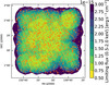 |
Fig. 1. Distribution of XMM-COSMOS AGN in the COSMOS field used in this study. Orange points mark the positions of 1130 AGNs with z = [0.1–2.5], while the background colors show the sensitivity map in the 0.5–2.0 keV band in erg cm−2 s−1 (Cappelluti et al. 2009). |
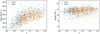 |
Fig. 2. Distribution of 2–10 keV luminosity (left) and host galaxy stellar mass (right) as a function of redshift for our sample of 1130 AGNs. Blue (orange) points show 632 (498) AGN with known spectroscopic (photometric) redshifts. |
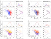 |
Fig. 3. Distribution in terms of M*, LX/M*, and redshift for XMM-COSMOS AGN with known spec-z (left panels) and spec-z + phot-z Pdfs (right panels). The low and high M* subsamples are created so that they have exactly the same specific BH accretion rate distribution (upper panels). A similar approach is used in terms of specific BH accretion rate (lower panels). For clarity, when the histograms match exactly, we have slightly offset the bins visually for the high subsample. |
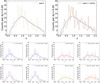 |
Fig. 4. Redshift distributions of data and random catalogs for our AGN subsamples. The colored histograms show the distribution of the redshifts in the data catalogs. The random redshifts (black histograms) are drawn from the smoothed redshift distribution of the data catalog using a Gaussian smoothing technique with σz = 0.3. |
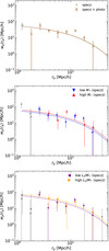 |
Fig. 5. Measured projected 2PCF for full sample and AGN subsamples. The errorbars correspond to 1σ estimated via the bootstrap method. The solid lines show the squared best-fit bias times the projected DM correlation function estimated at the mean redshift of the particular sample. The gray datapoints are not used in the fit due to a low number of pairs. The excess correlation at rp ∼ 15 h−1 Mpc is likely driven by large structure in the COSMOS field. |
Poissonian errors are readily assigned to the projected 2PCF. However, they are known to underestimate the errors. For this reason, we adopted a Bootstrap resampling technique by dividing the XMM-COSMOS survey into Nregion = 18 subregions (3 × 3 × 2 for RA, Dec, and comoving distance, respectively) of roughly equal comoving volumes. We resampled the regions Nrs = 100 times. In each of the resamplings, the regions were assigned different weights based on the number of times they were selected (Norberg et al. 2009). The elements of the covariance matrix C are then defined as
![$$ \begin{aligned} C_{ij} = \frac{1}{N_\mathrm{rs} } \sum _{k=1}^{N_\mathrm{rs} } \left[ w_{\mathrm{p},k}(r_{\mathrm{p},i}) - \left\langle w_{\rm p} \right\rangle (r_{\mathrm{p},i}) \right] \left[ w_{\mathrm{p},k}(r_{\mathrm{p},j}) - \left\langle w_{\rm p} \right\rangle (r_{\mathrm{p},j}) \right], \end{aligned} $$](/articles/aa/full_html/2019/09/aa35186-19/aa35186-19-eq48.gif)
where i and j refer to the ith and jth rp bins and the bar denotes the mean over Nregion resamples. The 1σ error for wp(rp, i) is the square root of the corresponding diagonal element, that is  .
.
4. Results
For each of the AGN subsamples, we estimated the projected 2PCF wp(rp) with rp = 1.0−100 h−1 Mpc using 12 logarithmic bins. We used one bin in the π direction, where the upper limit of this bin is dictated by πmax. In order to set πmax, we tried out all the values in the range πmax = 20–75 h−1 Mpc with an accuracy of Δπmax = 5 h−1 Mpc. For the full spectroscopic AGN sample, we found that the signal converges at πmax = 40 h−1 Mpc, which was adopted for all the subsamples. This value is similar to previous clustering studies involving XMM-COSMOS AGNs (Gilli et al. 2009; Allevato et al. 2011). The AGN projected 2PCF wp(rp) was then estimated using Eq. (7) and the 1σ bootstrap errors were estimated using Eq. (11). We show the estimated projected 2PCF for our subsamples in Fig. 5. Comparison between the spectroscopic subsamples and the specz+photz subsamples are shown in Figs. 5 (full) and 6 (M* and LX/M* subsamples).
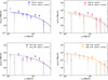 |
Fig. 6. Effect of including photometric redshifts as Pdfs in estimation of projected 2PCF. Triangles with different orientation mark the different AGN subsamples with spectroscopic redshifts only. Crosses show the projected 2PCF signal when including photometric redshifts as Pdfs. The lines show the squared best-fit bias times the projected DM correlation function. The bins have been slightly offset in the rp direction for clarity. |
We derived the best-fit large-scale bias, defined in Eq. (8), using χ2 minimization for rp = 1−30 h−1 Mpc. Furthermore, we utilized the inverse of the full covariance matrix C−1 and minimized χ2 = ΔTC−1Δ where Δ was with the same number of elements as the number of rp bins used in the fit. The symbol Δ is defined explicitly as  . With one free parameter, we estimated the 1σ errors on the best-fit bias, given by the lower and upper bounds of the region
  where ν = N − 1 is the number of degrees of freedom. To exclude noisy bins in the fit, we required that the number of pairs in each bin was > 16. The large-scale bias derived for all the XMM-COSMOS AGN subsamples are summarized in Table 1 and shown in Fig. 7.
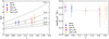 |
Fig. 7. Left: redshift evolution of bias for different XMM-COSMOS AGN subsamples. Crosses mark AGN subsamples where photometric redshifts are included in addition to spectroscopic redshifts. The gray dashed lines correspond to constant halo mass bias evolution b(z, Mhalo = const) for log Mhalo = 11.5, 12.0, 12.5, 13.0, 13.5 where Mhalo is given in units of h−1 M⊙. Right: corresponding typical AGN hosting halo mass evolution with redshift. For visual guidance, the dashed lines show the estimated mass of the halo for the full spectroscopic AGN sample. |
For the full spectroscopic AGN subsample (Fig. 5), we found a best-fit bias of  . Following the bias-mass relation described in van den Bosch (2002) and Sheth et al. (2001), this corresponds to a typical mass of the hosting halo of
  . It is important to note that in this work we define the typical mass explicitly as the DM halo mass which satisfies b = b(Mhalo) (e.g., Hickox et al. 2009; Allevato et al. 2016; Mountrichas et al. 2019). Albeit with large uncertainties, we find a small ≲1σ difference in the biases of the spectroscopic AGN subsamples split in terms of stellar mass (Fig. 5). The biases are
  for the low stellar mass and
  for the high stellar mass. However, it is worth noting that the two subsamples peak at different redshifts (z ∼ 1.0 versus z ∼ 1.4). We find no difference in terms of the typical masses of the hosting halos. For the M* subsamples, we find that excluding AGNs that are associated with groups has a greater effect on the measured best-fit bias of the low M* subsample. We measured
  (
( ) for the low (high) M* AGN subsample. This lower value for the bias could be an indication that AGNs in galaxies with lower stellar mass are more likely to be satellites in their DM halos compared to AGNs with higher stellar masses.
Moreover, we derived an AGN bias  (at z ∼ 0.9) and
  (z ∼ 1.5) for the low and high LX/M* subsamples, respectively (Fig. 5). No significant difference is observed in the typical masses of the hosting halos.
Similar results in terms of bias dependence on M* and LX/M* are found when using phot-z Pdfs in addition to any available spectroscopic redshifts. In particular, in our full AGN subsamples, an increase of ∼5% in the weighted number of AGNs introduces no systematic error in the estimation of the bias, but decreases the 1σ error of the bias by (δb1 − δb2)/δb1 ∼ 10% where δbi is the average error derived from the lower and upper limits of the bias (see Table 1). However, since including photometric redshifts does not change the conclusions drawn from our clustering measurements, we focus on the results from the AGN subsamples with known spectroscopic redshifts in the following sections.
5. Discussion
We performed clustering measurements of 1130 X-ray selected AGN in XMM-COSMOS at 0.1 < z < 2.5 (mean z ∼ 1.2) in order to study AGN clustering dependence on the host galaxy stellar mass and the specific BH accretion rate LX/M*. For our AGN subsamples, we find a typical DM halo mass ∼1013 h−1 M⊙ that roughly corresponds to group-sized environments. This is in agreement with similar studies using X-ray selected AGNs at similar redshifts (Coil et al. 2009; Allevato et al. 2011; Fanidakis et al. 2013; Koutoulidis et al. 2013) as well as at lower redshifts z < 0.1 (e.g., Krumpe et al. 2018; Powell et al. 2018). We also investigated including photometric redshifts as Pdfs in the analysis in addition to any available spectroscopic redshifts.
In COSMOS, Leauthaud et al. (2015) use weak lensing measurements on X-ray COSMOS AGN at z < 1 with log LX/erg s−1 = [41.5−43.5] and log M*/M⊙ = [10.5–12]. They infer that 50 percent of AGN reside in halos with log Mhalo/M⊙ < 12.5. This is not in agreement with the claim that X-ray AGN inhabit group-sized environments with masses ∼1013 M⊙. However, they also emphasize that due to the skewed tail in the halo mass distribution, the typical or the effective halo mass derived from clustering measurements may be markedly different from the median of the distribution.
In fact, they found an effective mass of Meff ∼ 1012.7 M⊙, which is close to the typical halo masses derived in this work. It is important to specify that they derived the effective halo mass from modeling the AGN halo occupation (see Sect. 5 in Leauthaud et al. 2015), which may differ from the typical halo mass inferred from the 2-halo term as in this work.
Also, they found that the effective DM halo mass of their AGN sample lies between the median and the mean values of the DM halo mass distribution, which are lower and higher than the effective DM halo mass, respectively. Given the statistics in our XMM-COSMOS AGN sample, we are not able to constrain the median or the mean of the DM halo mass distribution. In the future, this could be done with HOD modeling, provided that the 1-halo term is constrained.
Moreover, different cuts in luminosity and host galaxy mass may reflect in different hosting DM halo mass distributions. For instance, our sample of XMM-COSMOS AGN spans a range of host galaxy stellar masses log M*/M⊙ = [8–12], which also includes low-mass systems with masses < 1010.5 M⊙ (these are more likely satellite galaxies in galaxy groups) that also probe higher redshifts up to z = 2.5.
5.1. Clustering in terms of specific BH accretion rate
We divided the full sample in low and high specific BH accretion rate subsamples with the same M* distributions and find no significant clustering dependence on LX/M*, and thus the Eddington ratio. Krumpe et al. (2015) also found no dependence on λEdd for their sample of local (0.16 < z < 0.36) X-ray and optically selected AGN in the Rosat All-Sky Survey. They concluded that high accretion rates in AGN are not necessarily linked to high-density environments where galaxy interactions would be frequent. Our result provides further evidence that this is also true for non-local AGN at intermediate redshifts z ∼ 1. Mendez et al. (2016) studied the clustering of AGN in the PRIMUS and DEEP2 surveys (including the COSMOS field) at z ∼ 0.7 based on multiple selection criteria. In their X-ray selected AGN sample, they did not find a significant dependence on clustering in terms of specific BH accretion rate, which is in line with our results.
5.2. Clustering in terms of host galaxy stellar mass
We also studied the AGN clustering dependence on host galaxy stellar mass by probing the M*−Mhalo relation for active galaxies. In Fig. 8, we compare our results for XMM-COSMOS AGN with recent studies in literature using normal, non-active, galaxies. For our comparison purposes, we converted the results to our adopted h = 0.7 cosmology. Furthermore, we have converted the DM halo masses from different works to be consistent with our definition that is defined with respect to the mean density of the background. The blue curve shows the Moster et al. (2013)M*−Mhalo relation for central galaxies estimated using a multi-epoch abundance matching method which we have calculated at the mean redshift z ∼ 1.2 of our AGN sample. The orange curve shows the galaxy M*−Mhalo relation of Behroozi et al. (2013) at z ∼ 1.2. Coupon et al. (2015) estimated the M*−Mhalo relation in the CFHTLenS and VIPERS field at z ∼ 0.8 using constraints from several different methods including galaxy clustering. Compared to our AGN sample, their sample has a similar range in stellar mass and a slightly lower redshift. Results from HOD modeling of galaxy clustering in DEEP2 (Zheng et al. 2007) and the NMBS (Wake et al. 2011) at comparable redshifts (z ∼ 1.0–1.1) are shown as well. Using weak lensing methods, Leauthaud et al. (2015) studied a sample of moderate-luminosity AGN in COSMOS at a lower redshift z ∼ 0.66 than our sample. At M* > 1010.5 M⊙, they suggest that AGN populate similar DM halos as normal galaxies. Similarly, we find that high M* (≳1010.5 M⊙) XMM-COSMOS AGN follow the same M*−Mhalo relation as normal non-active galaxies. On the contrary, we estimated that low M* (≲1010.5 M⊙) AGN are more clustered than normal galaxies. Mountrichas et al. (2019) measured clustering of AGN from the XMM-XXL survey in terms of host galaxy properties (M*, SFR, and specific SFR) at z ∼ 0.8 and find a positive dependence on the environment with respect to M*. Our results at slightly higher redshift are in agreement with their measurements within errors (see Fig. 8).
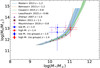 |
Fig. 8. M*−Mhalo relationship for our spectroscopic redshift AGN sample (stars) compared to previous studies in literature according to legend. For each of the M* subsamples, the horizontal errorbars represent one standard deviation of log M* of the sample. |
The M*−Mhalo relation obtained from our clustering analysis of XMM-COSMOS AGN is not consistent with results inferred for normal galaxies at similar redshifts, at least for the low M* bin. In fact, we find that AGN host galaxies with low M* reside in slightly more massive halos than normal galaxies of similar stellar mass. On the other hand, at high M*, our results are in good agreement with the M*−Mhalo relation of normal galaxies. As shown in Fig. 8, we do not expect the observed discrepancy at low M* to be caused by the different mean redshift of the two subsamples (z ∼ 1 and z ∼ 1.4). If we exclude AGN that are associated with galaxy groups from our M* subsamples, we see that this affects our low M* bin more, while the high M* bin is left relatively unchanged. This could indicate that XMM-COSMOS AGN with higher M* are more commonly found in the central galaxies of their respective halos. For lower M*, the fraction of AGNs as satellites would be higher. Nevertheless, excluding the galaxy groups from the analysis brings our result for the low M* closer to the M*−Mhalo of normal non-active galaxies.
It is important to note that our results for the M* subsamples include both type1 and type2 AGNs, that is AGNs regardless of obscuration are considered in the same subsample. With the limited sample size of XMM-COSMOS, we are not able to further divide the subsamples and examine the M*−Mhalo relation for type1 and type2 AGNs separately, to see whether there are any differences between these two populations. However, this issue can be revisited with Chandra COSMOS Legacy Survey AGNs.
6. Conclusions
We measured the clustering of XMM-COSMOS AGN in terms of host galaxy stellar mass M* and specific BH accretion rate LX/M*. Using these two quantities, we created AGN subsamples by splitting the full sample in terms of one quantity, while matching the distribution in the other. In addition, we investigated including AGNs with photometric redshifts as Pdfs in addition to AGNs with known spectroscopic redshifts. From our analysis, we make the following conclusions.
Firstly, XMM-COSMOS AGNs are highly biased with a typical DM halo mass of Mhalo ∼ 1013 h−1 M⊙, characteristic to group-sized environments and in broad agreement with previous results for moderate-luminosity X-ray selected AGN.
Secondly, we find no significant clustering dependence in terms of specific BH accretion rate, which is consistent with the idea that higher accretion rates in AGNs do not necessarily correspond to more dense environments. Also, we find no significant clustering dependence in terms of host galaxy stellar mass. By comparing our results with various M*−Mhalo relations found for normal non-active galaxies, we find that our low M* AGN subsample is more clustered than what is expected of normal galaxies at similar M*. We investigated this further by excluding AGNs that are associated with galaxy groups. We find that excluding objects in galaxy groups results in a lower AGN bias for the low M* AGN subsample, but this does not affect high M*. This could be due to a higher fraction of satellites for the lower stellar mass systems.
Lastly, our selected quality criterion for including additional photometric redshifts as Pdfs decreases the errors on the measured best-fit bias and does not introduce a bias to the clustering signal. Optimal quality cuts for including photometric redshifts will be studied in a future work.
Acknowledgments
We thank the referee for helpful comments that have improved this paper. AV is grateful to the Vilho, Yrjö and Kalle Väisälä Foundation of the Finnish Academy of Science and Letters. VA acknowledges funding from the European Union’s Horizon 2020 research and innovation programme under grant agreement No 749348. TM is supported by UNAM-DGAPA PAPIIT IN111379 and CONACyT 252531. RG acknowledges support from the agreement ASI-INAF n.2017-14-H.O.
References
- Alexander, D. M., & Hickox, R. C. 2012, New Astron. Rev., 56, 93 [NASA ADS] [CrossRef] [Google Scholar]
- Allevato, V., Finoguenov, A., Cappelluti, N., et al. 2011, ApJ, 736, 99 [NASA ADS] [CrossRef] [Google Scholar]
- Allevato, V., Finoguenov, A., Hasinger, G., et al. 2012, ApJ, 758, 47 [NASA ADS] [CrossRef] [Google Scholar]
- Allevato, V., Finoguenov, A., Civano, F., et al. 2014, ApJ, 796, 4 [NASA ADS] [CrossRef] [Google Scholar]
- Allevato, V., Civano, F., Finoguenov, A., et al. 2016, ApJ, 832, 70 [NASA ADS] [CrossRef] [Google Scholar]
- Behroozi, P. S., Wechsler, R. H., & Conroy, C. 2013, ApJ, 770, 57 [NASA ADS] [CrossRef] [Google Scholar]
- Bongiorno, A., Merloni, A., Brusa, M., et al. 2012, MNRAS, 427, 3103 [NASA ADS] [CrossRef] [Google Scholar]
- Brusa, M., Civano, F., Comastri, A., et al. 2010, ApJ, 716, 348 [NASA ADS] [CrossRef] [Google Scholar]
- Cappelluti, N., Hasinger, G., Brusa, M., et al. 2007, ApJS, 172, 341 [NASA ADS] [CrossRef] [Google Scholar]
- Cappelluti, N., Brusa, M., Hasinger, G., et al. 2009, A&A, 497, 635 [NASA ADS] [CrossRef] [EDP Sciences] [Google Scholar]
- Cappelluti, N., Allevato, V., & Finoguenov, A. 2012, Adv. Astron., 2012, 853701 [NASA ADS] [CrossRef] [Google Scholar]
- Civano, F., Marchesi, S., Comastri, A., et al. 2016, ApJ, 819, 62 [NASA ADS] [CrossRef] [Google Scholar]
- Coil, A. L., Georgakakis, A., Newman, J. A., et al. 2009, ApJ, 701, 1484 [NASA ADS] [CrossRef] [Google Scholar]
- Cooray, A., & Sheth, R. 2002, Phys. Rep., 372, 1 [NASA ADS] [CrossRef] [Google Scholar]
- Coupon, J., Arnouts, S., van Waerbeke, L., et al. 2015, MNRAS, 449, 1352 [NASA ADS] [CrossRef] [Google Scholar]
- Croom, S. M., Boyle, B. J., Shanks, T., et al. 2005, MNRAS, 356, 415 [NASA ADS] [CrossRef] [Google Scholar]
- daÂngela, J., Shanks, T., Croom, S. M., et al. 2008, MNRAS, 383, 565 [NASA ADS] [CrossRef] [Google Scholar]
- Davis, M., & Peebles, P. J. E. 1983, ApJ, 267, 465 [NASA ADS] [CrossRef] [Google Scholar]
- Eisenstein, D. J., & Hu, W. 1999, ApJ, 511, 5 [NASA ADS] [CrossRef] [Google Scholar]
- Fanidakis, N., Georgakakis, A., Mountrichas, G., et al. 2013, MNRAS, 435, 679 [NASA ADS] [CrossRef] [Google Scholar]
- Georgakakis, A., Mountrichas, G., Salvato, M., et al. 2014, MNRAS, 443, 3327 [NASA ADS] [CrossRef] [Google Scholar]
- Gilli, R., Zamorani, G., Miyaji, T., et al. 2009, A&A, 494, 33 [NASA ADS] [CrossRef] [EDP Sciences] [Google Scholar]
- Gozaliasl, G., Finoguenov, A., Tanaka, M., et al. 2019, MNRAS, 483, 3545 [NASA ADS] [CrossRef] [Google Scholar]
- Hasinger, G., Cappelluti, N., Brunner, H., et al. 2007, ApJS, 172, 29 [NASA ADS] [CrossRef] [Google Scholar]
- Hasinger, G., Capak, P., Salvato, M., et al. 2018, ApJ, 858, 77 [NASA ADS] [CrossRef] [Google Scholar]
- Hickox, R. C., Jones, C., Forman, W. R., et al. 2009, ApJ, 696, 891 [Google Scholar]
- Koutoulidis, L., Plionis, M., Georgantopoulos, I., & Fanidakis, N. 2013, MNRAS, 428, 1382 [NASA ADS] [CrossRef] [Google Scholar]
- Koutoulidis, L., Georgantopoulos, I., Mountrichas, G., et al. 2018, MNRAS, 481, 3063 [NASA ADS] [CrossRef] [Google Scholar]
- Krumpe, M., Miyaji, T., & Coil, A. L. 2014, Multifrequency Behaviour of High Energy Cosmic Sources, 71 [Google Scholar]
- Krumpe, M., Miyaji, T., Husemann, B., et al. 2015, ApJ, 815, 21 [NASA ADS] [CrossRef] [Google Scholar]
- Krumpe, M., Miyaji, T., Coil, A. L., & Aceves, H. 2018, MNRAS, 474, 1773 [NASA ADS] [CrossRef] [Google Scholar]
- Landy, S. D., & Szalay, A. S. 1993, ApJ, 412, 64 [NASA ADS] [CrossRef] [Google Scholar]
- Leauthaud, A. J., Benson, A., Civano, F., et al. 2015, MNRAS, 446, 1874 [NASA ADS] [CrossRef] [Google Scholar]
- Marchesi, S., Civano, F., Elvis, M., et al. 2016, ApJ, 817, 34 [NASA ADS] [CrossRef] [Google Scholar]
- Marulli, F., Veropalumbo, A., & Moresco, M. 2016, Astron. Comput., 14, 35 [NASA ADS] [CrossRef] [Google Scholar]
- Mendez, A. J., Coil, A. L., Aird, J., et al. 2016, ApJ, 821, 55 [NASA ADS] [CrossRef] [Google Scholar]
- Merloni, A., Alexander, D. A., Banerji, M., et al. 2019, The Messenger, 175, 42 [NASA ADS] [Google Scholar]
- Miyaji, T., Zamorani, G., Cappelluti, N., et al. 2007, ApJS, 172, 396 [NASA ADS] [CrossRef] [Google Scholar]
- Moster, B. P., Naab, T., & White, S. D. M. 2013, MNRAS, 428, 3121 [NASA ADS] [CrossRef] [Google Scholar]
- Mountrichas, G., Georgakakis, A., Menzel, M.-L., et al. 2016, MNRAS, 457, 4195 [NASA ADS] [CrossRef] [Google Scholar]
- Mountrichas, G., Georgakakis, A., & Georgantopoulos, I. 2019, MNRAS, 483, 1374 [NASA ADS] [CrossRef] [Google Scholar]
- Norberg, P., Baugh, C. M., Gaztañaga, E., & Croton, D. J. 2009, MNRAS, 396, 19 [NASA ADS] [CrossRef] [Google Scholar]
- Powell, M. C., Cappelluti, N., Urry, C. M., et al. 2018, ApJ, 858, 110 [NASA ADS] [CrossRef] [Google Scholar]
- Ross, N. P., Shen, Y., Strauss, M. A., et al. 2009, ApJ, 697, 1634 [NASA ADS] [CrossRef] [Google Scholar]
- Salvato, M., Hasinger, G., Ilbert, O., et al. 2009, ApJ, 690, 1250 [CrossRef] [Google Scholar]
- Salvato, M., Ilbert, O., Hasinger, G., et al. 2011, ApJ, 742, 61 [NASA ADS] [CrossRef] [Google Scholar]
- Scoville, N., Aussel, H., Brusa, M., et al. 2007, ApJS, 172, 1 [NASA ADS] [CrossRef] [Google Scholar]
- Sheth, R. K., Mo, H. J., & Tormen, G. 2001, MNRAS, 323, 1 [NASA ADS] [CrossRef] [Google Scholar]
- van den Bosch, F. C. 2002, MNRAS, 331, 98 [Google Scholar]
- Wake, D. A., Whitaker, K. E., Labbé, I., et al. 2011, ApJ, 728, 46 [NASA ADS] [CrossRef] [Google Scholar]
- Zheng, Z., Coil, A. L., & Zehavi, I. 2007, ApJ, 667, 760 [NASA ADS] [CrossRef] [Google Scholar]
All Tables
All Figures
|
Fig. 1. Distribution of XMM-COSMOS AGN in the COSMOS field used in this study. Orange points mark the positions of 1130 AGNs with z = [0.1–2.5], while the background colors show the sensitivity map in the 0.5–2.0 keV band in erg cm−2 s−1 (Cappelluti et al. 2009). |
| In the text | |
|
Fig. 2. Distribution of 2–10 keV luminosity (left) and host galaxy stellar mass (right) as a function of redshift for our sample of 1130 AGNs. Blue (orange) points show 632 (498) AGN with known spectroscopic (photometric) redshifts. |
| In the text | |
|
Fig. 3. Distribution in terms of M*, LX/M*, and redshift for XMM-COSMOS AGN with known spec-z (left panels) and spec-z + phot-z Pdfs (right panels). The low and high M* subsamples are created so that they have exactly the same specific BH accretion rate distribution (upper panels). A similar approach is used in terms of specific BH accretion rate (lower panels). For clarity, when the histograms match exactly, we have slightly offset the bins visually for the high subsample. |
| In the text | |
|
Fig. 4. Redshift distributions of data and random catalogs for our AGN subsamples. The colored histograms show the distribution of the redshifts in the data catalogs. The random redshifts (black histograms) are drawn from the smoothed redshift distribution of the data catalog using a Gaussian smoothing technique with σz = 0.3. |
| In the text | |
|
Fig. 5. Measured projected 2PCF for full sample and AGN subsamples. The errorbars correspond to 1σ estimated via the bootstrap method. The solid lines show the squared best-fit bias times the projected DM correlation function estimated at the mean redshift of the particular sample. The gray datapoints are not used in the fit due to a low number of pairs. The excess correlation at rp ∼ 15 h−1 Mpc is likely driven by large structure in the COSMOS field. |
| In the text | |
|
Fig. 6. Effect of including photometric redshifts as Pdfs in estimation of projected 2PCF. Triangles with different orientation mark the different AGN subsamples with spectroscopic redshifts only. Crosses show the projected 2PCF signal when including photometric redshifts as Pdfs. The lines show the squared best-fit bias times the projected DM correlation function. The bins have been slightly offset in the rp direction for clarity. |
| In the text | |
|
Fig. 7. Left: redshift evolution of bias for different XMM-COSMOS AGN subsamples. Crosses mark AGN subsamples where photometric redshifts are included in addition to spectroscopic redshifts. The gray dashed lines correspond to constant halo mass bias evolution b(z, Mhalo = const) for log Mhalo = 11.5, 12.0, 12.5, 13.0, 13.5 where Mhalo is given in units of h−1 M⊙. Right: corresponding typical AGN hosting halo mass evolution with redshift. For visual guidance, the dashed lines show the estimated mass of the halo for the full spectroscopic AGN sample. |
| In the text | |
|
Fig. 8. M*−Mhalo relationship for our spectroscopic redshift AGN sample (stars) compared to previous studies in literature according to legend. For each of the M* subsamples, the horizontal errorbars represent one standard deviation of log M* of the sample. |
| In the text | |
Current usage metrics show cumulative count of Article Views (full-text article views including HTML views, PDF and ePub downloads, according to the available data) and Abstracts Views on Vision4Press platform.
Data correspond to usage on the plateform after 2015. The current usage metrics is available 48-96 hours after online publication and is updated daily on week days.
Initial download of the metrics may take a while.